Analyzing the Hydroelectricity Variability on Power Markets from a System Dynamics and Dynamic Systems Perspective: Seasonality and ENSO Phenomenon

Abstract

In this paper, the variations in hydropower generation are addressed considering the seasonality and ENSO (El Niño-Southern Oscillation) episodes. The dynamic hypothesis and the stock-flow structure of the Colombian electricity market were analyzed. Moreover, its dynamic behavior was analyzed by using Dynamic Systems tools aimed at providing deep insight into the system. The MATLAB/Simulink model was used to evaluate the Colombian electricity market. Since we combine System Dynamics and Dynamic Systems, this methodology provides a novel insight and a deeper analysis compared with System Dynamics models and can be easily implemented by policymakers to suggest improvements in regulation or market structures. We also provide a detailed description of the Colombian electricity market dynamics under a broad range of demand growth rate scenarios inspired by the bifurcation and control theory of Dynamic Systems.

1. Introduction

Electricity generation has become one of the most important topics because of not only the growing demand but also its effects on the environment. Globally, the main source of electricity generation is derived from fossil fuels [1], a non-renewable resource that gives rise to a large amount of greenhouse gases that pollute the environment. Thus, renewable energy is currently considered an alternative source of generation to counteract the undesired effects caused by fossil fuel technologies [2]. In this sense, the deployment of environmentally friendly sources of electricity generation grows in the short and medium terms [3], which, in turn, may require the adaptation of the electricity markets to their gradual implementation. On the one hand, any source of generation dependent on intermittent and seasonal resources can be considered as a variable generation technology [4], which lacks a consistent source of energy. On the other hand, sources of generation that totally or partially depend on climatic conditions are cataloged as seasonal. Unlike intermittent technologies, seasonal resources are characterized by undergoing reductions or increases in their generation due to the climatic seasons, but never stop generating electricity. In general terms, the variability in renewable generation and its effects on the electricity markets have been addressed in several countries using different modeling approaches [5,6,7], but System Dynamics (SD) in combination with Dynamic Systems (DS), which can expand the analysis spectrum, has never been used to evaluate such variability.

In recent years, SD has been used to investigate complex systems [8,9,10,11]. SD methodology can provide modeling or capturing variables that the physics laws fail to perform. Consequently, SD has become a powerful modeling technique since its foundation in the mid-1950s by Professor Jay Forrester of the Massachusetts Institute of Technology [12]. This approach can be a useful mathematical modeling technique for understanding and discussing complex issues and problems in several areas [13]. Nevertheless, the classical SD software restricts the detailed analysis of complex systems since it only enables the investigation of time series or limited sensitivity studies.

Consequently, investigation trends reveal that SD is complemented with other modeling techniques to improve the analysis and achieve a higher degree of knowledge of the systems [8,14]. However, a limited number of works complemented SD with the theory of DS [15,16,17,18,19,20]; for this reason, and considering that the SD methodology can be applied in practically all research areas, we think that the combination of SD and DS can offer valuable insight into complex system analysis. Simple SD models can be easily transformed into a DS model and analytically solved; however, most real systems are highly complex, making their analytical study challenging. However, by using numerical DS tools, a hybrid SD/DS approach can be developed as demonstrated in our previous work [20], which is extended here by desegregating variables, incorporating the ENSO phenomenon, and developing a more advanced sensitivity analysis by considering the ENSO phenomenon and the chaos theory. Our proposed methodology can be applied to not only energy systems but also in any SD model by following the steps explained in Section 3. Indeed, the results discovered by our proposed SD/DS approach in the Colombian power market may be relevant to international power markets that have a similar energy matrix and follow the supply and demand laws.

Conversely, although Colombia’s weather reflects a periodic behavioral pattern throughout the year, the ENSO phenomenon alters such dynamics and disturbs, to some extent, the cyclical behavior of dry and wet seasons [21,22]. Therefore, the water contributions of the Colombian rivers used to power the hydroelectricity plants might be highly increased or reduced, according to the presence of La Niña or El Niño events, respectively. Our model considers the availability factor of the hydroelectricity generation ($a{f}_v$) to represent such hydroelectricity climatic dynamics. Thus, we propose to capture, through $a{f}_v$, not only the seasonality but also the ENSO phenomenon to incorporate more realistic characteristics affecting the Colombian electricity supply and demand in our model.

Accordingly, we formulated a deterministic function that can approximate the real characteristics of the water contributions of the Colombian rivers for modeling the seasonality and ENSO phenomenon, which has been altering the Colombian seasonality since 1950 [23]. However, in some cases, the ENSO phenomenon had a stronger influence than others. Colombia has been through several electricity risks because of the appearance of strong El Niño events, such as 1991–1992, 1997, 2008, and 2015–2016. Indeed, the worst-case scenario for Colombia was reported in 1991–1992 since there were several rationing events programmed by the government.

Thus, we obtained the historical mean water contributions from 2000 to 2016 to observe the general hydroelectricity climatic dynamics of the Colombian rivers. In this work, we obtained the complete historical synthetic series to show how seasonality and the past ENSO phenomenon have affected water resources in Colombia over a time span of 17-years and validated the renewable generation dynamics of 2017, 2018, and 2019, as explained in Section 5.1. Technically, we first extracted the real data from the XM’s (company that manages the Colombian electricity market) records [24] in terms of energy inputs and then computed the corresponding $a{f}_v$ (in percentage), as shown in Figure 6 by the red line. Note that over the past years, the $a{f}_v$ has experienced situations both with great potential and water scarcity. In some cases, very low levels were seen because of strong El Niño events.

2. The Colombian Electricity Market

2.1. Real System Overview

Colombia has abundant natural resources, reflected in its electricity sources mostly dominated by hydropower generation with a nearly 70% (≈11611.1 MW) of its capacity, followed by fossil fuel plants (29%, ≈4833 MW) and non-conventional renewable sources (1%, ≈151 MW); hence, Colombia is mainly driven by hydroelectric and thermal power plants. For our model, we assumed that the electricity demand ($ed$) of the Colombian electricity market could be met with hydroelectric and thermal power plants.

Since the liberalization of the energy market in 1990 to promote private investment, Colombia has achieved a clear legal framework, fair competition conditions, stability for investors, and improvements to the security of supply [25]. Inspired by the British model, the Colombian electricity sector has been reformed over the years, and it is more efficient and reliable today because of the well-developed laws that promote a good market competition.

In general terms, the dispatch process to meet the $ed$ is based on the lowest price offers. It means that the sources of generation that can produce power at the lowest price possible are placed at the top level of the electricity matrix to supply the $ed$. If the $ed$ is not fully met, the next source of generation in the electricity matrix is called to supply more electricity. This process continues until the $ed$ is covered. Once the total $ed$ is met, the system sets the market price according to the price offer established by the last source of generation used. In other words, the dynamics of the Colombian electricity market are governed by the well-known supply and demand forces.

Furthermore, the operation of the hydroelectricity plants is highly dependent on the level of their reservoirs, whereas thermal plants rely on fuel availability. In fact, thermal plants in Colombia are much more reliable and considered as a support for hydroelectricity generation since fuel availability is not a problem. On the contrary, hydroelectric plants can be strongly affected by weather conditions considering that dry periods have been observed nowadays.

Although Colombia has prioritized clean energy production, a 70% installed capacity of variable generation (hydroelectric plants) can indirectly cause other issues. In fact, this hydroelectricity variability can be more pronounced when other market variables are altered, such as the growth rate of demand ($GRD$). Thus, we aimed to address how changes in the $GRD$ can affect the performance of the Colombian electricity market, which is highly dependent on variable and permanent generation plants.

2.2. Simulation Overview

The results described in the present paper were obtained by combining the SD and DS perspectives; accordingly, two computer programs were developed. First, under the SD approach, the dynamic hypothesis of the Colombian electricity sector was identified. Second, the corresponding stock-flow diagram was derived from the causal loop one to perform a more detailed quantitative analysis. Finally, the stock-flow structure was transformed into a Simulink block diagram to analyze the system from a DS perspective.

Hence, to investigate our system in detail, it is necessary to follow one of these two steps once the stock-flow structure has been constructed:

• Obtain the dynamic equations, and perform an analytical study if possible. Then, program the equations in any programming language (determined by the modeler depending on system requirements, simplicity, interface, user friendliness, performance, and accuracy, among others), and finally, develop any strategy of analysis on the basis of the existing DS tools.
• Inspired by the control theory, transform the stock-flow structure (obtained with the SD approach) into an analogous block diagram using Simulink. Then, develop any strategy of analysis in a normal script of MATLAB on the basis of the existing DS tools.

In this paper, we followed the second step for simplicity, because (i) an analytical study is very hard or impossible to apply since the solution of the dynamic equations can only be approximated using numerical methods, and (ii) for creating a friendly simulation environment, such that the SD community finds practical, broadly applicable, more accurate and intuitive than existing ones. Accordingly, we created the analogous block diagram in Simulink and then implemented different tools of analysis in a single script of MATLAB, which has a simple design that is easy to modify and extend.

3. SD/DS Modeling

3.1. Dynamic Hypothesis

Our electricity market model seeks to show the causalities among the different Colombian market variables, $GRD$ scenarios, and the imminent effects of seasonality and ENSO phenomenon in the generation process. As shown in Figure 1, the dynamic hypothesis [26] comprises three balance loops. $B_1$ represents the dynamic interaction of the demand side variables, whereas $B_2$ and $B_3$ represent the supply side associated with hydropower (V) and fossil fuel (P) generation, respectively. As mentioned above, the Colombian electricity generation is dominated by hydroelectricity, which is considered a variable source of generation because it is annually affected by the climate variability of the country; therefore, (V) in Figure 1 refers to the variable hydropower generation. In the same manner, the second-largest source of generation (thermal power) is considered a permanent source of generation considering that its availability remains constant; consequently, (P) is used to refer to this technology.

As one can see, the balance loop $B_1$ indicates that increasing the values of market price incentives reductions in energy consumption, which in turn affects the reserve margin positively. Similarly, when the electricity market is experiencing a reserve margin shortfall, $B_2$ explains that consumers must pay a higher price. However, this turns out in greater returns on investment for the producers. Clearly, these incentivize the expansion of both variable and permanent capacity, since the market price causalities affect not only the balance loop $B_2$ but also $B_3$; therefore, the reserve margin is affected positively. Note that this increase in the reserve margin balances the subsequent causalities.

3.2. Stock-Flow Diagram

The second step of our work implies, as the SD approach suggests [12], a stock and flow building process to perform a quantitative analysis. This process allows us to transform the causal loop diagram into a stock-flow diagram, which can describe the system in more detail involving the formulation of the dynamic equations.

First, the supply side of (P) generation (referring to all Colombian’s fossil fuel power plants) involves the expansion of this sector, comprised of two stock variables, its capacity under construction, and installed capacity (Figure 2). The construction of new plants depends on the investment decision of the producers, which is determined by their returns on investment. The higher the electricity tariff, the higher the investment incentives for new capacity. In Colombia, the highest price is usually reached when thermal plants are used to produce electricity, since the cost of fuel is more expensive than producing energy with water resources.

Similarly, as shown in Figure 3, the supply side of (V) generation (for all Colombian hydroelectric power plants) is also associated with the expansion of this sector. Installing new capacity is highly dependent on generating producer profit. In other words, high electricity tariffs benefit the capacity under construction because producers’ desired for investment is stimulated, which eventually increases the installed capacity of hydropower generation.

Conversely, the thermal and hydroelectric power plants will eventually become obsolete, affecting the installed capacity negatively since they will need to be removed from the system. In fact, the dynamics of the installed capacity in both technologies are affected similarly by two flows, the retirement of old plants and the retirement of initial ones, as shown in Figure 2 and Figure 3. The flow retirement of initial plants is used to remove the initial value of the installed capacity, i.e., the current state of the permanent installed capacity, or the current state of the variable installed capacity. The initial installed capacity refers to all hydroelectric and thermal power plants which were previously built and are still in operation. However, determining their lifetime is challenging mainly because most of them became part of the system in different years, and others do not have accurate information of when they started to participate in the Colombian electricity market; consequently, they are smoothly removed from the installed capacity, considering the average lifetime of a general hydroelectricity (or thermal) power plant, using a first-order delay [27]. In contrast, to gain accuracy in the model, new installed capacity is removed from the system, once the power plants become obsolete, using a pipeline delay (infinite order delay) through the flow retirement of old plants [27].

Figure 4 shows that the power demand plays an important role in market dynamics. The interaction among generators, which compete for providing energy services at the price set by the market, influences the reserve margin of the electricity system. Furthermore, the market price formation depends on not only the reserve margin, which set a rationing price when its level reaches a critical value, but also the last technology of generation participating in the dispatch process to meet the total $ed$. Moreover, this market price is slightly delayed since the consumers in Colombia perceive the current electricity price with a certain lag. Consequently, and as it is expected in the real system, the market price, together with the elasticity of demand (also known as price elasticity of demand) in Colombia [28], causes either a positive or negative effect on the demand behavior. In fact, the effect of price on demand ($epd$) depends entirely on the market price, delayed market price, and elasticity of demand (see also Equation (A6)). The $epd$ has been modeled as an index that can take values below and under 1 to capture how changes in the market price stimulate changes in the $ed$. An $epd>1$ means a decrease in the market price, which in turn, influences an increase in the $ed$; in contrast, an $epd<1$ means an increase in the market price, which causes a decrease in the $ed$, demonstrating how the supply and demand forces work in power markets [29,30,31,32].

Finally, the dispatch process is considered in Figure 5. Under the assumption of a perfect electricity market competition, the firms cannot influence the market price. In fact, the dispatching merit order is determined by the market, which sorts the available technologies of generation according to their marginal costs, from the cheapest to the most expensive. This means that the first power plants called to dispatch their energy are those that offer the cheapest electricity price. Once the supply equals the demand, the market price is set by the most expensive technology of generation, which is in operation at that time. This price determines the returns on investment, which eventually influence the system capacity expansion, as it is included in the supply side modeling. Moreover, in the dispatch side, some other variables are determined; for example, the utilization factor, which is a percentage measure of the participation of power plants in the dispatch process, is used to directly affect the returns on investment together with the market price. In other words, the amount of energy dispatched by each technology per its generation capacity (generation) provides a rate of usage of that technology (utilization factor), which is used to compute its return on investment. Conversely, the generation capacity depends on the source of generation, essentially, its availability. For example, thermal power plants, are considered as the permanent sources of generation as their availability is mostly constant and only restricted by fuel availability; consequently, the availability factor can be kept constant. However, the generation capacity of hydroelectric power plants is highly determined by either the amount of water in the reservoirs or the flow of rivers, both of which are strongly affected by weather conditions; consequently, its availability factor cannot be constant but is modeled by considering the water contributions of Colombian rivers. Although this availability factor could reach values > 100%, the capacity factor always reduces it because of the technical constraints of power plants.

3.3. Block Diagrams of Simulink

As a final step in the modeling process, we transformed the above stock-flow structure into a block diagram of Simulink to investigate our problem with the support of DS tools. As we already discussed above, the transformation of a stock-flow structure into a block diagram of Simulink is very intuitive and does not require us to program numerical methods to solve ODEs, and Simulink provides more advantages than other SD software packages, such as Vensim, Powersim, and Stella. Once we have the model in Simulink, any strategy of analysis can be implemented for investigating its dynamics because DS tools can be easily implemented or applied in Simulink than having the normal system equations programmed in MATLAB, C++, or Python. The detailed explanation of the Simulink block diagrams is provided in Appendix A.

4. Modeling the Seasonality and ENSO Phenomenon

Figure 6 shows the real variability of the hydropower generation (red line), which reproduces both the seasonality and ENSO phenomenon and has a high random component. Accordingly, involving probabilistic techniques would be appropriate for modeling such random variability. Nevertheless, we continued looking for solutions involving deterministic equations or functions to model the variability, as stated in our previous paper [20]. Therefore, we used a chaotic attractor, which represents the ENSO dynamics. More precisely, the Lorenz attractor is used to model the ENSO phenomenon, whereas seasonality is represented by Equation (1). Others have also shown that strange attractors (or chaos) influence the Colombian hydroclimatology [21], confirming the existence of chaotic deterministic components in the Colombian hydrology.

Thus, we incorporated the ENSO phenomenon in $a{f}_v$ through a Lorenz attractor and seasonality. The latter has been modeled using Equation (1) [20]. See the resulting behavior of Equation (1) (the Colombian seasonality) in [20].

$$a{f}_v=1.01+0.47sin(2\pi t-0.45\pi )\times cos(2\pi t-0.45\pi )+0.25sin(2\pi t-0.55\pi )$$

(1)

Generally, the seasonality effects tend to be more pronounced when the ENSO appears; for example, dry seasons might bring droughts, and wet seasons, floods. Thus, we added the ENSO component with the seasonality component so that $a{f}_v$ can contain both dynamics. Indeed, it has been shown that El Niño phenomenon is a season-induced chaotic resonance between the ocean and the atmosphere [22]. The Lorenz attractor can be shown by Equation (2) [33]:

$$\begin{array}{c}\dot{x}=a(y-x)\hfill \\ \dot{y}=x(b-z)-y\hfill \\ \dot{z}=xy-cz\hfill \end{array}$$

(2)

where a, b, and c are parameters used to generate chaos dynamics (

Table 1. Parameter values of the Lorenz attractor.

Parameter	Value
a	10
b	28
c	2.6667
$x\left(0\right)$	10
$y\left(0\right)$	5
$z\left(0\right)$	20

) and x, y, and z are the state variables [33].

Accordingly, to obtain a more realistic hydropower generation variability, we implemented both the Lorenz attractorusing Equation (2) and the seasonality using Equation (1) in $a{f}_v$. The stock-flow structure, the Simulink block diagram, and the parameter values are shown in Figure 7 and Figure 8 and Table 1, respectively.

To test our proposed $a{f}_v$, we fixed the initial conditions, a, b, and c of the Lorenz attractor to exhibit the classical butterfly effect. Then, we selected one of its three state variables to represent the ENSO phenomenon by considering their individual dynamics; therefore, z was selected since it exhibited a behavior like the real $a{f}_v$. Finally, we ran the model and obtained the synthetic series shown in Figure 6 through the dashed blue line. As can be seen, the simulated signal agrees with the real one, and the $MAPE$ = 11.35%. The $MAPE$ measures the prediction accuracy of a forecasting method and stands for mean absolute percentage error. It is defined as $\frac{1}{n}{\sum }_{t=1}^n\left|\frac{y_t-\widehat{y_t}}{y_t}\right|\ast 100$, where n is the number of observations, $y_t$ is the real value, and $\widehat{y_t}$ is the estimated value of the time series.

The simulated $a{f}_v$ (dashed blue signal) was obtained by using only a determined and fixed set of initial conditions. However, as the chaos theory states, even slight changes in the initial conditions of a chaotic system result in very different behaviors. Thus, the simulated dashed blue line in Figure 6 is only one possible reality of the Colombian $a{f}_v$, so by varying the initial conditions of the Lorenz attractor, infinite realities can be obtained.

5. Results

5.1. Model Validation

The results of the validation process are out of the scope of this work. However, the model robustness was tested by following the method explained elsewhere [34,35]. We also applied a highly advanced sensitivity analysis to our model and validated the tests.

Moreover, we computed the basic time series of our proposed model in Vensim, MATLAB, and Simulink to verify their accuracy, and all three of them showed good agreement. To further test the accuracy of our simulation model, we decided to run it starting from 2017, so that part of the simulation time series and sensitivity analysis can be contrasted with the real data of the Colombian electricity market. Consequently, we found that our simulations completely reflect the real system. In much more detail, we found that unmet $ed$ events were expected to occur in 2019, as shown in Figure 9d. Moreover, we found that for some $GRD$ values, months of electricity rationing were expected to occur in 2019. According to the upper right diagram of Figure 14, these months might be January, February, November, and December. If we look at the 3-D diagram of Figure 14, January 2019 has the worst-case scenario since it has a nearly 72% probability of occurrence. In contrast to the real system, we found that 2019 was a critical year in Colombia since it was informed by one of the utilities in April 2018 that Hidroituango (a new 2400 MW hydropower plant expected to enter into the system in 2019 [36]) had some construction problems and needed to be delayed for 2–3 years [37]. Of course, this was a big perturbation that caused a supply risk during 2019, especially in January and February, and November and December [38], as suggested in our simulation model. All these supported the reliability of our simulation model. Here, it is important to highlight that our model does not predict the Hidroituango perturbation and that we only withdrew the Hidroituango capacity from our model to observe if our model was going to be able to reproduce the real dynamics of the Colombian power market from 2017 to 2019.

Considering all these validation processes, and that 2019 has already passed, below we focus on the results starting from 2020.

5.2. Simulation of the Colombian Electricity Market

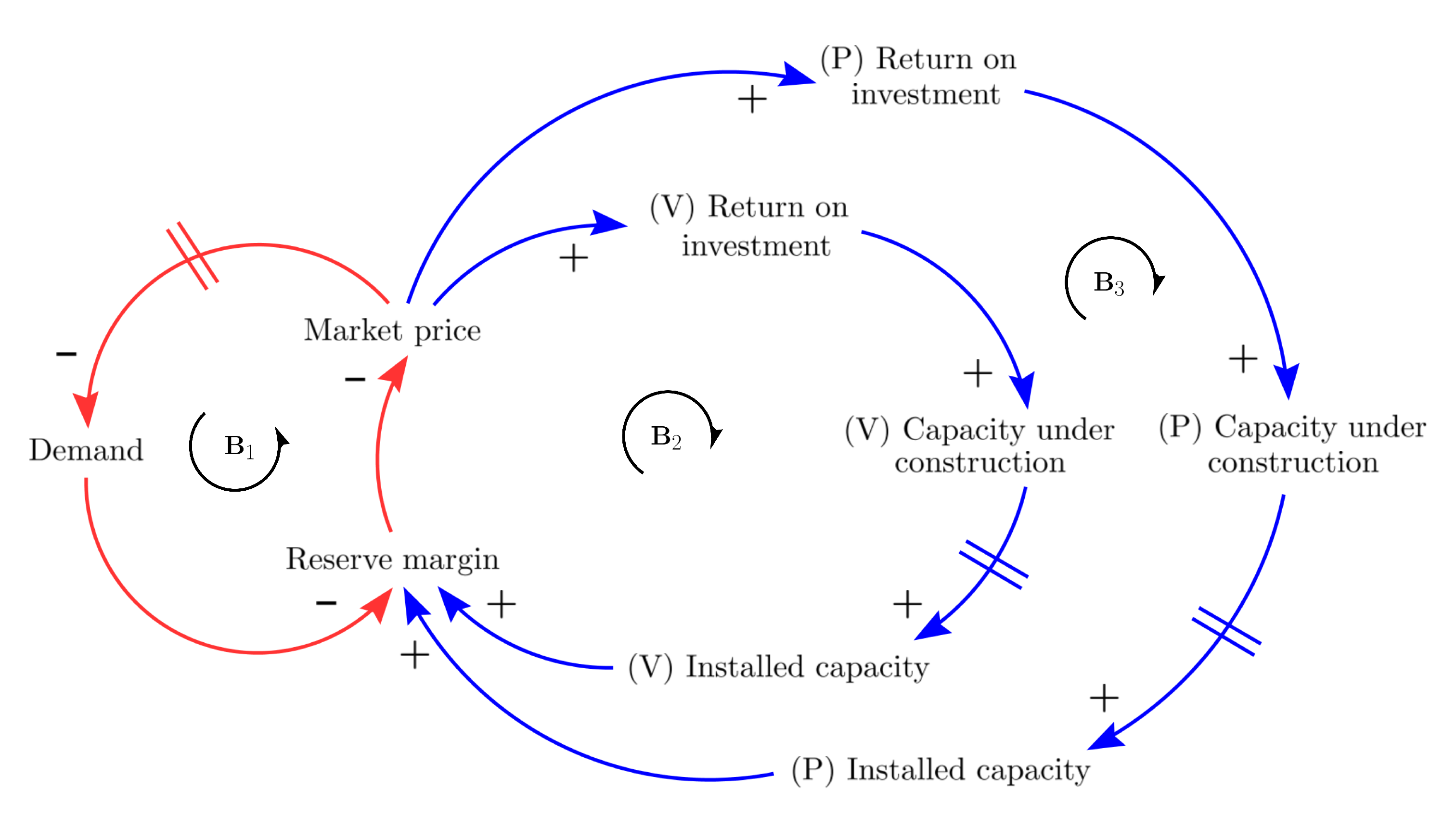
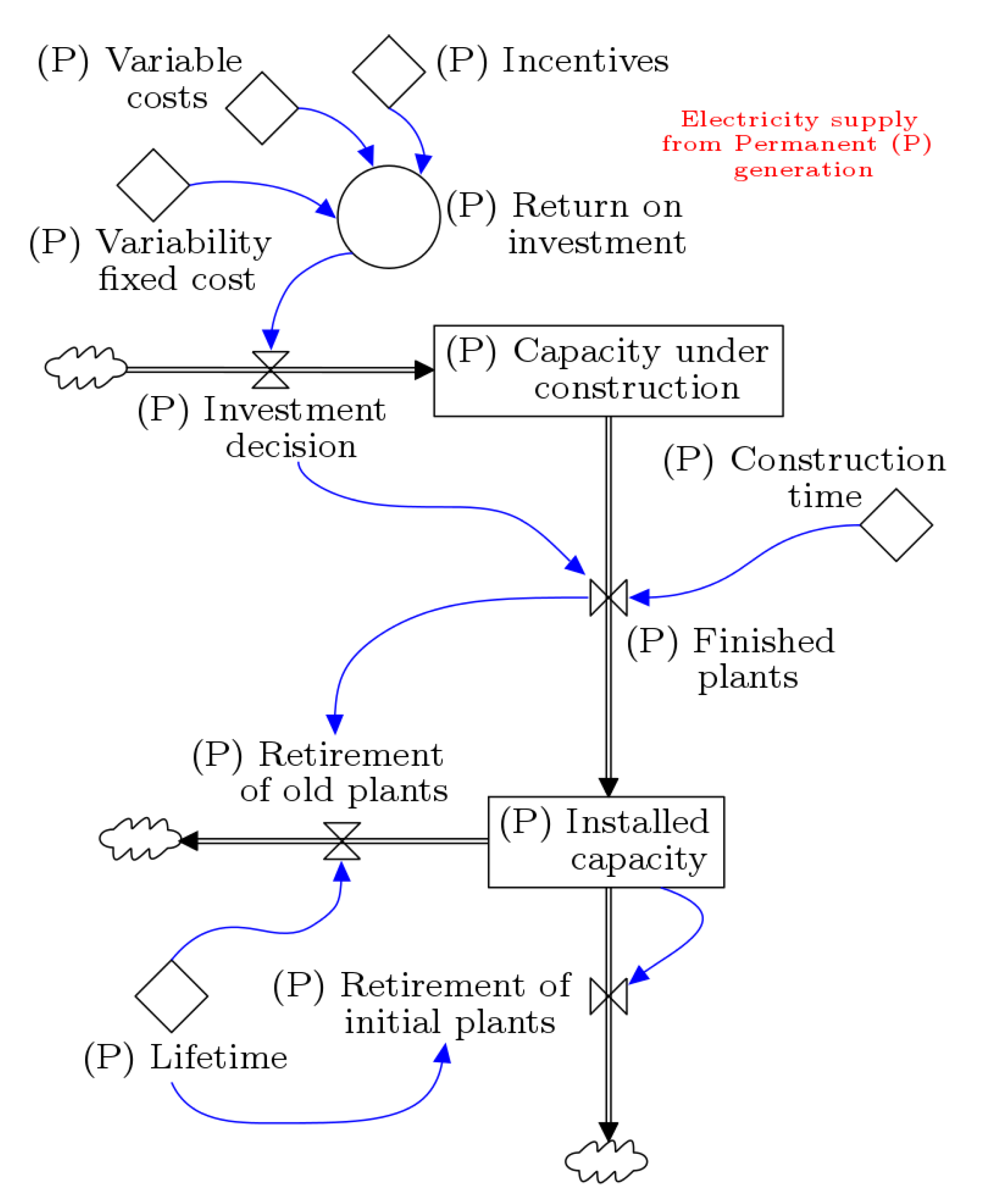
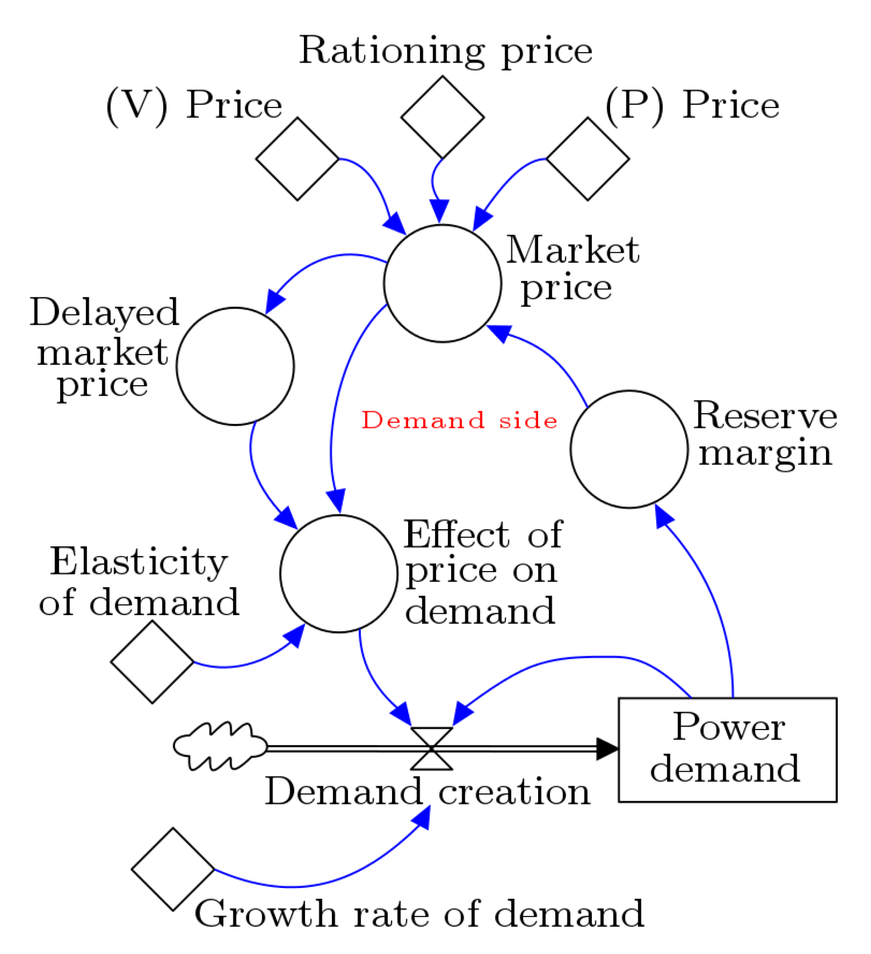
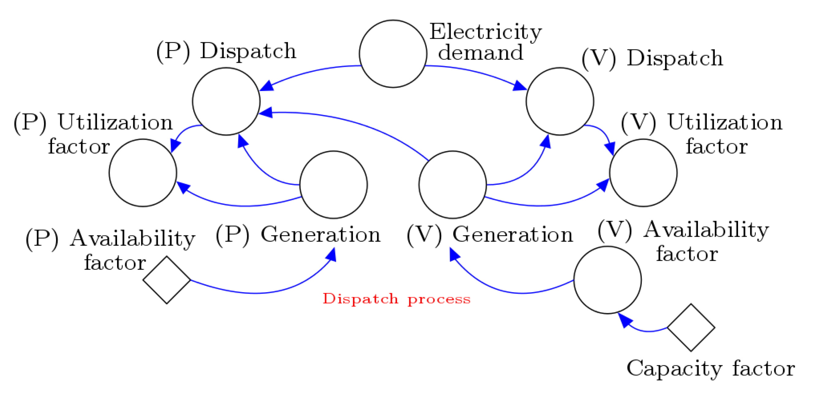
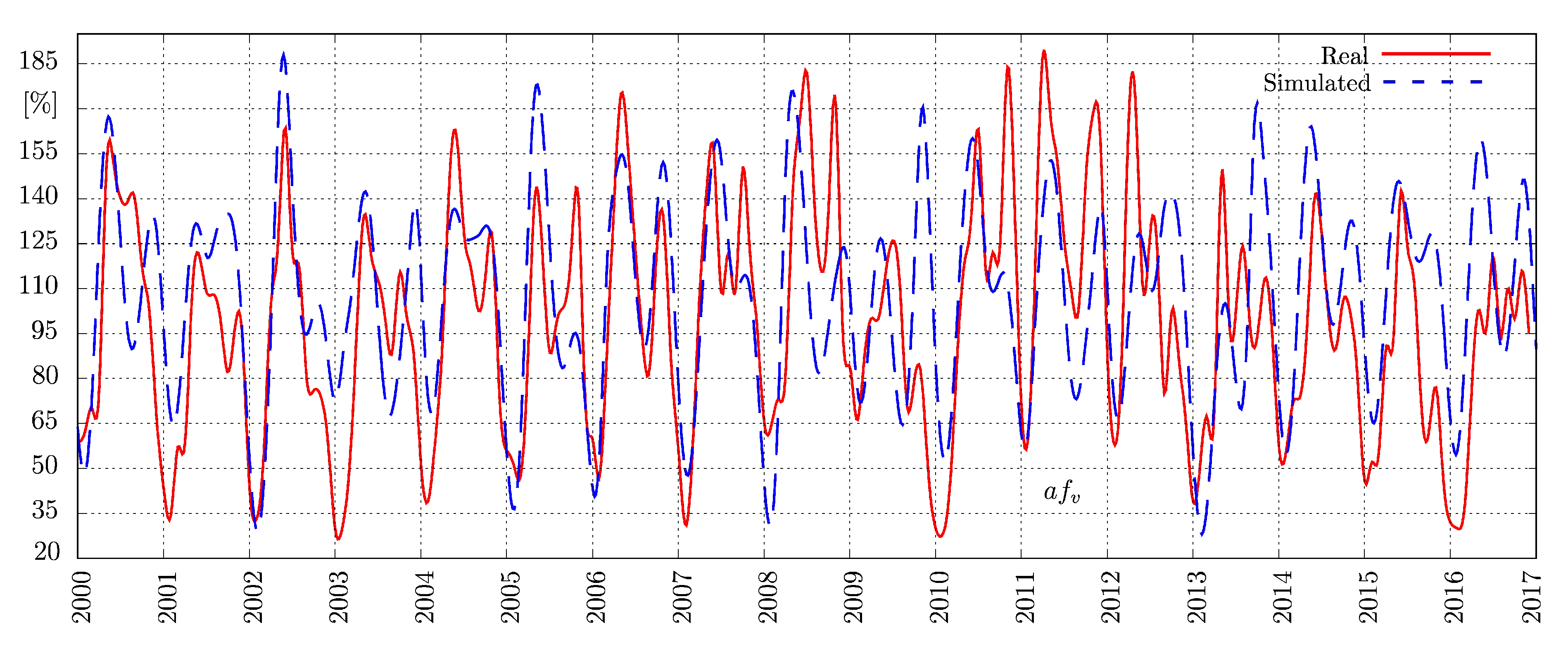
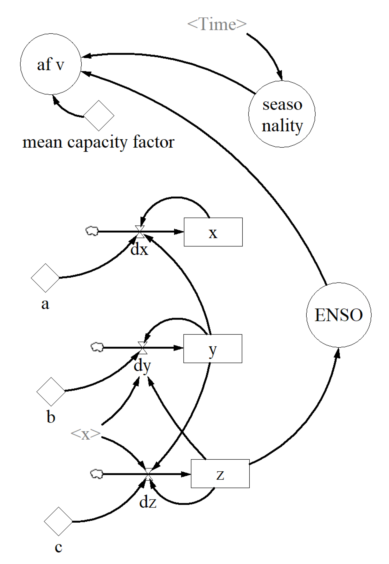
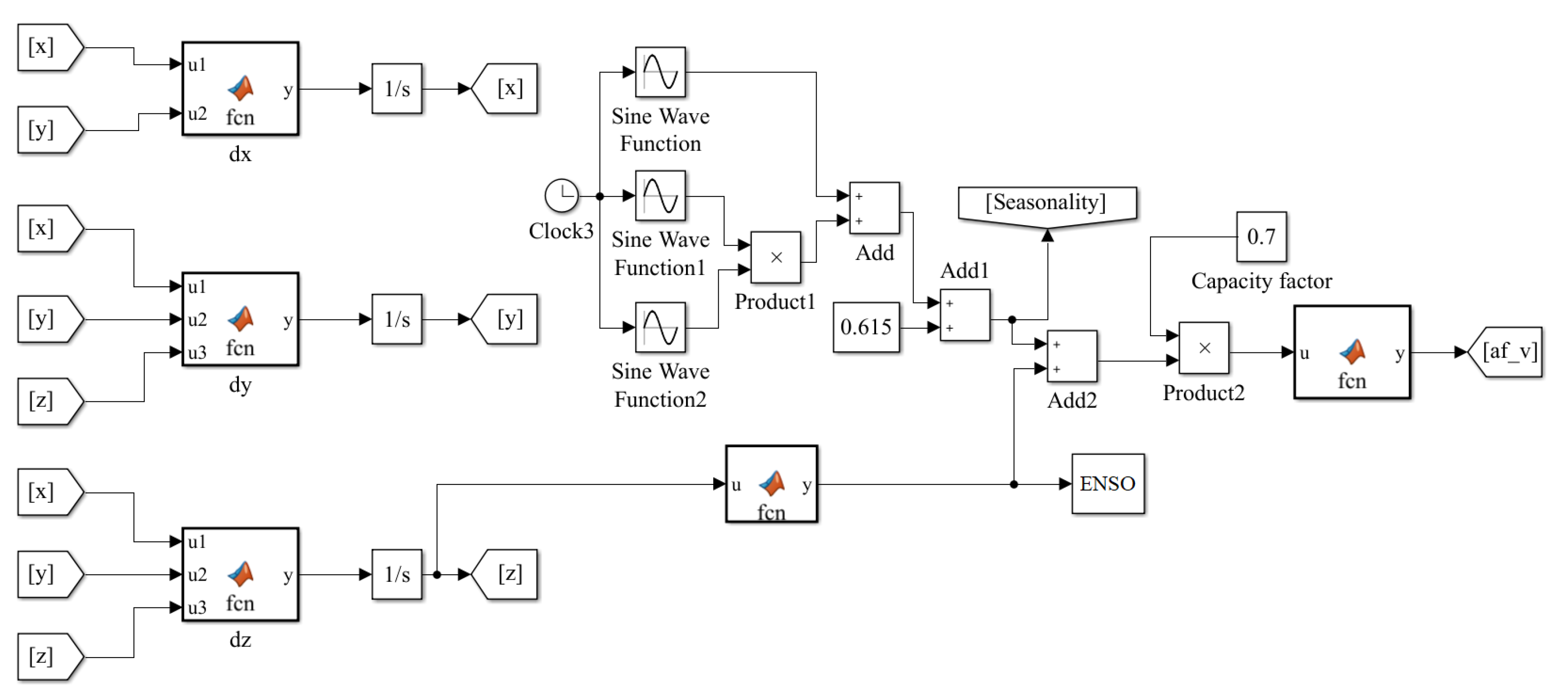
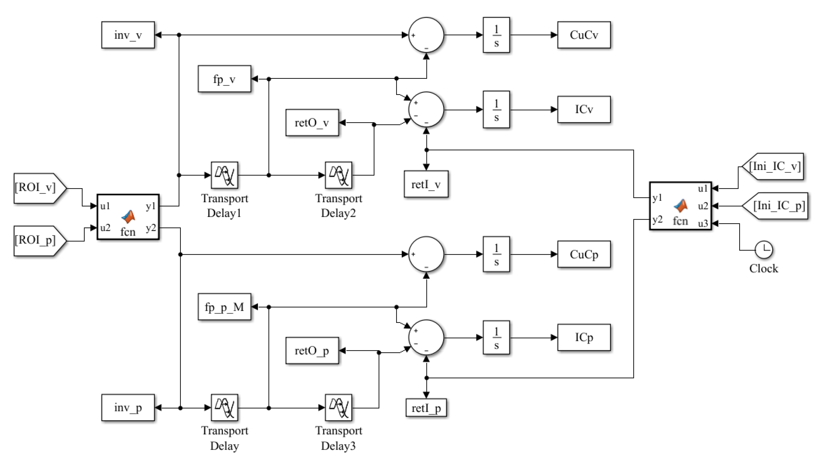
In this section, both the seasonality and ENSO phenomenon are considered for modeling the variability of hydropower plants as explained before. The stock-flow structure is shown in Figure 2, Figure 3, Figure 4 and Figure 5. The Colombian parameter values used in this section are shown in

Table 2. Parameters used in the model based on the Colombian electricity sector.

Parameter	Value
Construction time ($CT$)	5 yr
Lifetime ($LT$)	30 yr
Growth rate of demand ($GRD$)	0.039
Variable cost ($VC$)	150 COP/kWh
Incentives (I)	0 COP/kWh
Variability fixed cost ($VFC$)	60 COP/kWh
$y\left(0\right)$	15,521 MW
$z\left(0\right)$	9320 MW
$x\left(0\right)$	0 MW
Minimum price ($MP$)	35 COP/kWh
Maximum increase of price ($MIP$)	350 COP/kWh
Elasticity of demand ($\epsilon$)	$-0.3$

.

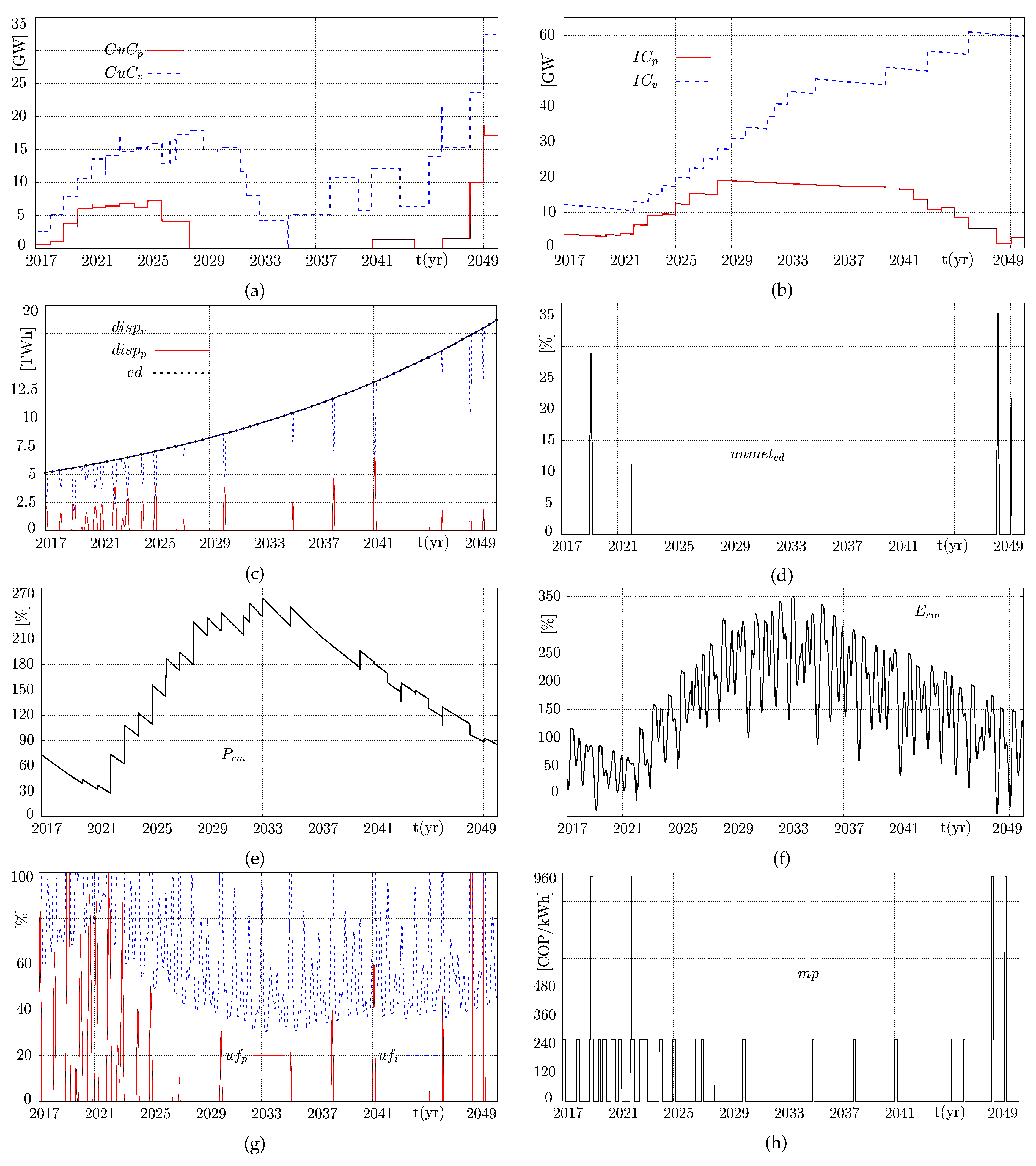
Now let us show how the seasonality and the ENSO phenomenon affect the main characteristics of the simplified Colombian electricity market in Figure 9. These simulations were obtained by considering the BaU scenario, i.e., with the current policies and average population growth. As can be seen, the chaotic component of the ENSO phenomenon has been introduced to the overall market dynamics. Here, the ENSO phenomenon gives rise to several unexpected situations. Generally, the variability of the hydropower generation produced by seasonality and ENSO phenomenon forces the system to use more thermal generation not only in the short and long run but also over the middle term. Clearly, the El Niño phenomenon makes the electricity supply dependent on more permanent generation along the 33-years of simulation. The short and long runs are also the two most critical situations. Figure 9d shows that unmet $ed$ events are expected in 2022, 2048, and 2049, whereas the security of supply is maintained in the middle run.

In Figure 9a,b, the dynamics of the capacity under construction of the permanent ($Cu{C}_p$) and variable ($Cu{C}_v$) generation and the installed capacity of the permanent ($I{C}_p$) and variable generation ($I{C}_v$) are shown, respectively. Similarly, Figure 9c shows the interaction of the electricity dispatch of the permanent ($dis{p}_p$) and variable ($dis{p}_v$) generation for meeting the $ed$. As a result of this process, it is measured the unmet $ed$ ($unme{t}_{ed}$), as shown in Figure 9d. In this sense, the reserve margin can also be observed in Figure 9e,f since it can be measured in terms of its power ($P_{rm}$) and energy ($E_{rm}$). Additionally, the dynamics of the utilization factor of the permanent ($u{f}_p$) and variable ($u{f}_v$) generation can also be observed in Figure 9g. Finally, the market price behavior of the system is observed in Figure 9h.

Nevertheless, the previous simulations were obtained for only one initial condition of the Lorenz attractor, that is, only one possible reality. As we discussed above, chaotic attractors are very sensitive to changes in their initial conditions. Therefore, every change in the initial condition of the Lorenz attractor can be a different possible reality and therefore in $a{f}_v$. Thus, we can change the initial condition of z and generate very different synthetic series. However, the question arises as to how many synthetic series should be computed.

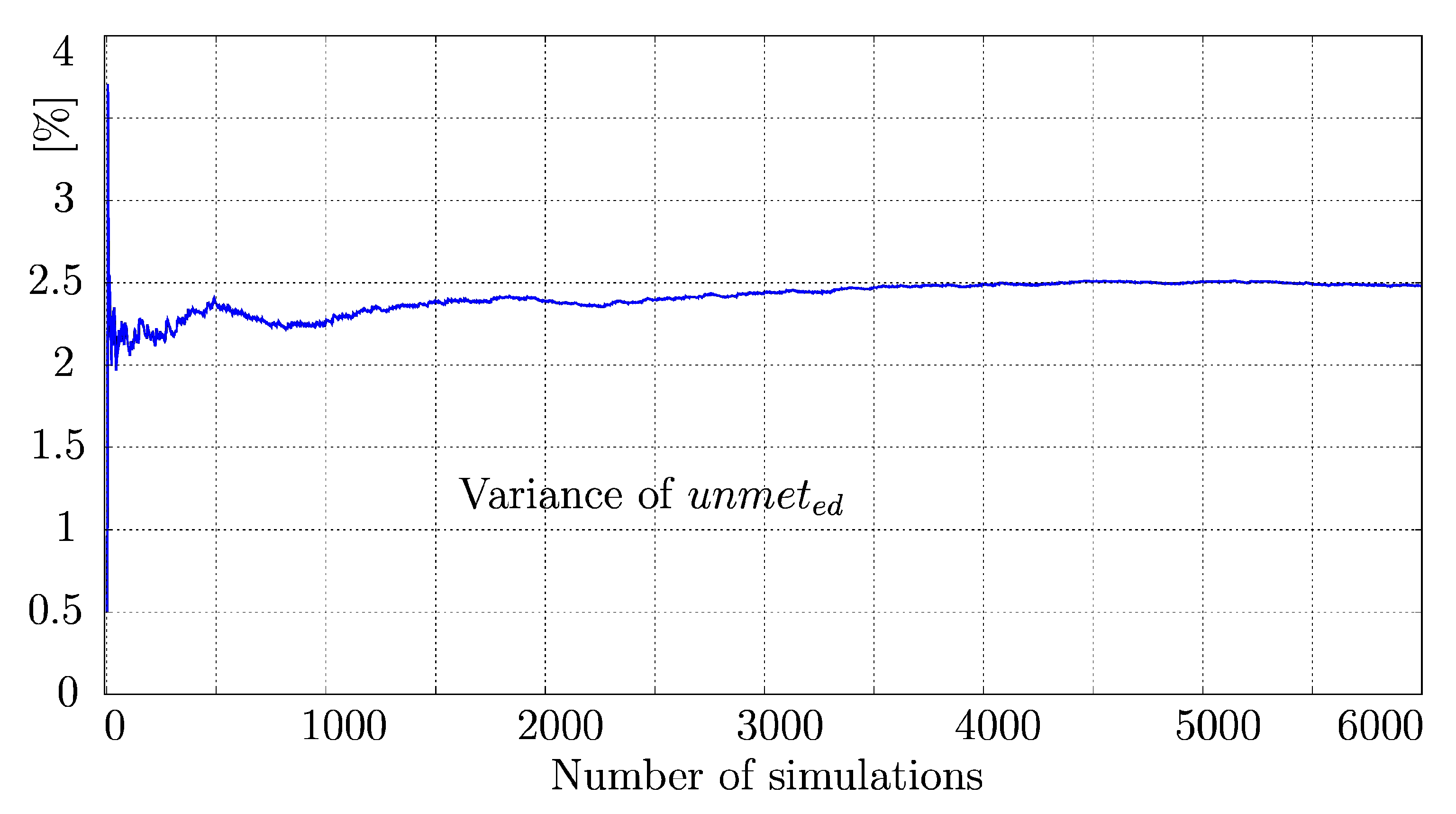
To address this question, we computed the variance of one of the market variables under many different initial conditions (synthetic series). Then, we determined the number of synthetic series that should be computed to always guarantee the generation of different synthetic series or realities of $a{f}_v$.

In this context, let us show Figure 10, which shows the variance of the $unme{t}_{ed}$. Note that by setting different initial conditions to the Lorenz attractor, different scenarios or the behaviors of the $unme{t}_{ed}$ were obtained, especially in the first 2000 simulations. After 4000 simulations, although the initial condition was still being changed, the variance reached an equilibrium point. Thus, irrespective of the continued variation in the initial condition of z, the resulting synthetic series do not change significantly. Consequently, by simulating the electricity market model up to 4000 times, we guarantee 4000 different synthetic series. In fact, we can consider such 4000 possible realities for studying different $GRD$ scenarios.

5.3. Demand Growth Scenarios: A Bifurcation Perspective

So far, the BaU scenario under seasonality and ENSO phenomenon is explained with only one possible reality out of 4000. However, population, economic growth, energy efficiency improvements, and diffusion of self-generation with solar panels, are all key influences in energy demand. Therefore, in this section, we provide low and high demand growth scenarios, as well as a broad spectrum of $GRD$ scenarios by simulating 4000 possible realities of the Colombian power market.

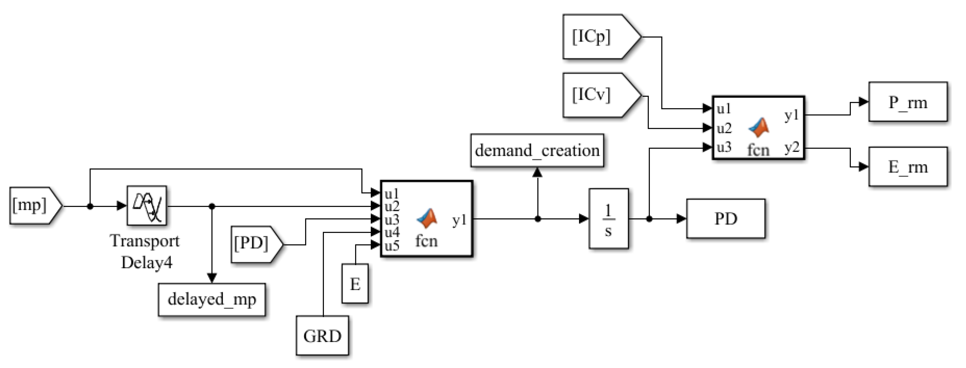
To perform this study, we used the parameter $GRD$ shown in Figure 4. This parameter represents the population and economic growth, which directly influences the $ed$ dynamics. Accordingly, the $GRD$ was varied from −0.04 to 0.1. For each $GRD$ value, our model was simulated 4000 times. However, for representation purposes only, the average dynamics of all 4000 synthetic series are illustrated, which enables us to observe a smoother behaviour of the system variables. Considering that the simulation of such a huge number of synthetic series is limited by computational power, we only computed 200 $GRD$ scenarios. This means that we computed a total of 800,000 synthetic series.

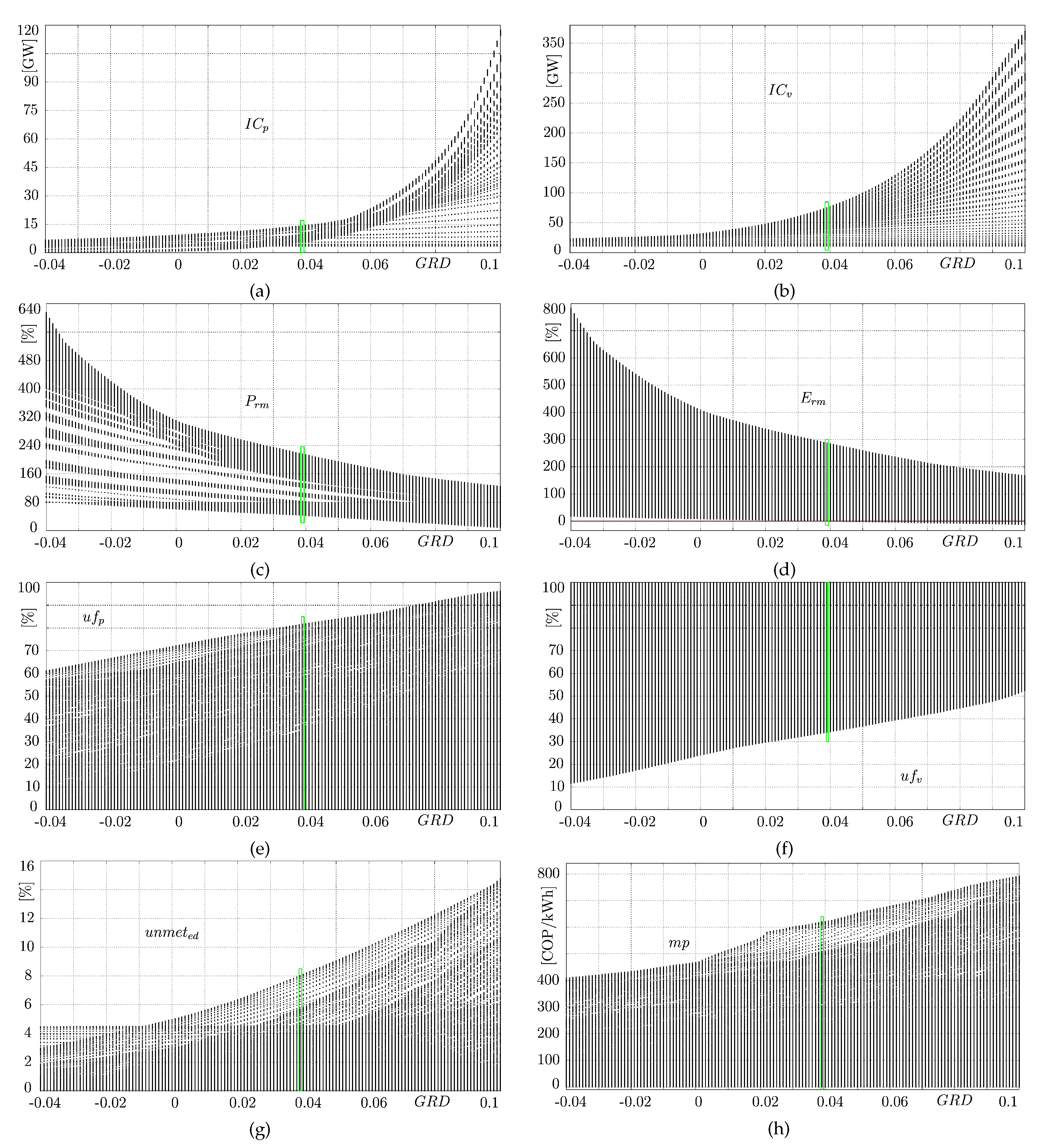
A more advanced sensitivity analysis diagrams are shown in Figure 11 based on the concept of bifurcation diagrams. Notably, our model is characterized for exhibiting an infinite transient behavior (stable solutions are not achievable) due to the strong dependence on continuously growing investment decisions and demand. Nevertheless, the concept of bifurcation diagrams is used for not only the last values of the synthetic series (as commonly done for physical systems), but also the short, middle, and long run values of the simulations, as stated in [19,39], as a map of all possible scenarios.

As shown in Figure 11a,b, the seasonality and ENSO phenomenon do not significantly influence the dynamics of $I{C}_v$ and $I{C}_p$; chaotic or variability components are not displayed in both diagrams. Only a continuously growing pattern can be observed as $GRD$ increased. Since all synthetic series were averaged, the sensitivity diagrams show a smoother behavior pattern. In fact, as we explained before, because of the merit order effect, the $I{C}_v$ is always above the $I{C}_p$. This suggests that, regardless of the variability of hydropower generation and the $GRD$ scenario, renewable and fossil fuel capacities tend to increase in the short term and in the long term. Nevertheless, the hydropower capacity always grows faster than the thermal capacity for well-known environmental reasons.

Note that for the Colombian case (green rectangle), $I{C}_p$ and $I{C}_v$ reach maximum values of 14 and 72 GW, respectively, close to the possible reality shown in Figure 9b. $I{C}_v$ reaches this value almost at the end of the simulation (2046), whereas $I{C}_p$, near 2028. Thus, the variability imposed by the ENSO episodes is very strong and thus forces the thermal capacity to grow and the hydropower capacity to decrease correspondingly. The electricity market tries to mitigate such strong variability by using more permanent or thermal generation. Accordingly, we can expect to have the same conclusion for all $GRD$ scenarios.

Conversely, note that negative values of the $GRD$ do not incentivize the expansion of both $I{C}_p$ and $I{C}_v$, which is explained by the continuous drop in consumption due to decreasing $ed$. Moreover, by increasing the value of the $GRD$, one can see a clear growth in both installed capacities. Particularly, the $I{C}_v$ exhibits exponential growth. The $I{C}_p$, conversely, presents a slower exponential growth more concentrated for large values of $GRD$, and no intermittent complex dynamics are observed because the permanent capacity is larger and thus less critical values of $E_{rm}$ are exhibited or, at least, $E_{rm}$ does not abruptly change (see Figure 11d). Both the nearly smooth growth of $I{C}_p$ and $I{C}_v$ and the larger share of permanent generation give rise to a less variable $E_{rm}$.

Figure 11c shows that $P_{rm}$ shows positive margins for all $GRD$ values. However, although more permanent capacity is installed when the ENSO is part of the model, its stronger variability leads $P_{rm}$ to more critical instances as $GRD$ increases; consequently, negative $E_{rm}$ values are more likely to occur for larger $GRD$ scenarios, as shown in Figure 11d. Almost all positive $GRD$ scenarios lead to a similar negative $E_{rm}$ value, which is more pronounced around $GRD$ = 0.09. The question arises whether it occurs in the short or long run, which we discuss in the following section.

Furthermore, when the $ed$ is decreasing ($GRD$< 0), both $P_{rm}$ and $E_{rm}$ grow higher than other $GRD$ scenarios, but critical values are reached as well at some time in the simulation. In fact, when we further increase the $GRD$, $P_{rm}$ and $E_{rm}$ smoothly decrease and become more critical. For the Colombian case, particularly, $E_{rm}$ might cross the red line in 2021–2022, 2048, and 2049, as shown in Figure 9d. The Colombian case is part of the most dangerous $GRD$ scenarios seen in this figure (for $GRD$ = 0.02 onward).

Our electricity market model, which now incorporates the ENSO phenomenon, exhibits $unme{t}_{ed}$ events for all $GRD$ scenarios, as illustrated in Figure 11g. Note that for some parameter values $unme{t}_{ed}$ could be very high, whereas others could be low. In Colombia, the $GRD$ is close to 0.039, and as shown in Figure 9d, it might be possible to have $unme{t}_{ed}$ ≈ 12%, 35%, and 22% in 2022, 2048, and 2049, respectively. However, these values correspond to only one of the 4000 possible realities computed; therefore, after averaging all the 4000 synthetic series of $unme{t}_{ed}$, a maximum value of 8% is obtained for the Colombian case, as illustrated in Figure 11g, which we further investigated in this work. In fact, the risk to have $unme{t}_{ed}$ events is imminent. Indeed, it might be the worst if the $GRD$ increases. It appears that the only way to avoid such critical situations is by installing new permanent or variable capacity before 2021, only by doing so, Colombia might change its energy future landscape. Colombia urgently needs a new capacity to change its overall energy future prospective. Considering that it is expected to have a larger $GRD$ over time, Colombia could be subjected to an increasing risk of undergoing significant $unme{t}_{ed}$ episodes.

From Figure 11h, one can see that $unme{t}_{ed}$ events can also be detected from the $mp$. Recall that when $E_{rm}$ becomes zero or negative, the system sends a signal of setting a $RAP$ in the $mp$; therefore, one can see in the $mp$ that the signal of $RAP$ is set in all $GRD$ scenarios since the maximum price reached by the system is above $P_p$. In other words, the $mp$ takes values between $P_p$ and $P_v$, and at some time, it also takes a $RAP$. For this reason, the sensitivity diagram captures values ranging from 0 to 800 COP/kWh. The smaller the value of the $GRD$ scenario, the cheaper the $mp$ will be for consumers. Obviously, a small $GRD$ value leads to fewer rationing episodes over time, which in turn, guarantees cheaper prices for consumers. The question arises whether the $RAP$ is set in the short or long term, which shall be further investigated, but it can be partly inferred from the $unme{t}_{ed}$ dynamics explained above.

Additionally, Figure 11e,f illustrate the participation of each technology of generation in the dispatch merit order. As shown, hydroelectricity power plants ($u{f}_v$) are used in all $GRD$ scenarios ranging from no less than 12% and up to 100%. However, this interval of participation shrinks as the $GRD$ further increases, basically because it is necessary to mitigate the ENSO variability by installing more permanent capacity and reducing the variable one. For instance, in the Colombian case $u{f}_v$ ranges from 35% to 100% depending on different conditions, whereas for $GRD$ = 0.1, one would expect $u{f}_v$ ranging from 53% to 100%, 18% less participation than the Colombian scenario. The thermal plants are not used at their full potential ($u{f}_p$ = 100%) because more thermal and less variable capacities are installed so that less participation from permanent generation is needed to meet the $ed$. However, for negative values of $GRD$, the participation of renewable power plants can be larger since the appearance of rationing events is less unlikely.

Evidently, the larger the values of $GRD$, the more electricity is needed to be able to meet the increased $ed$; therefore, the participation of thermal power plants is larger for those $GRD$ scenarios. The thermal power plants are less used for all $GRD$ scenarios (a large permanent capacity together with a significant variable one can meet the required $ed$ sufficiently), for $u{f}_p$ between 0% and 95%. Under the current market structure, the full potential of thermal plants is not necessary for supporting the hydropower generation, meeting the $ed$, and avoiding the rationing events; however, it can be unavoidable because of the complex dynamics of the hydropower variability, as shown in Figure 11d,g.

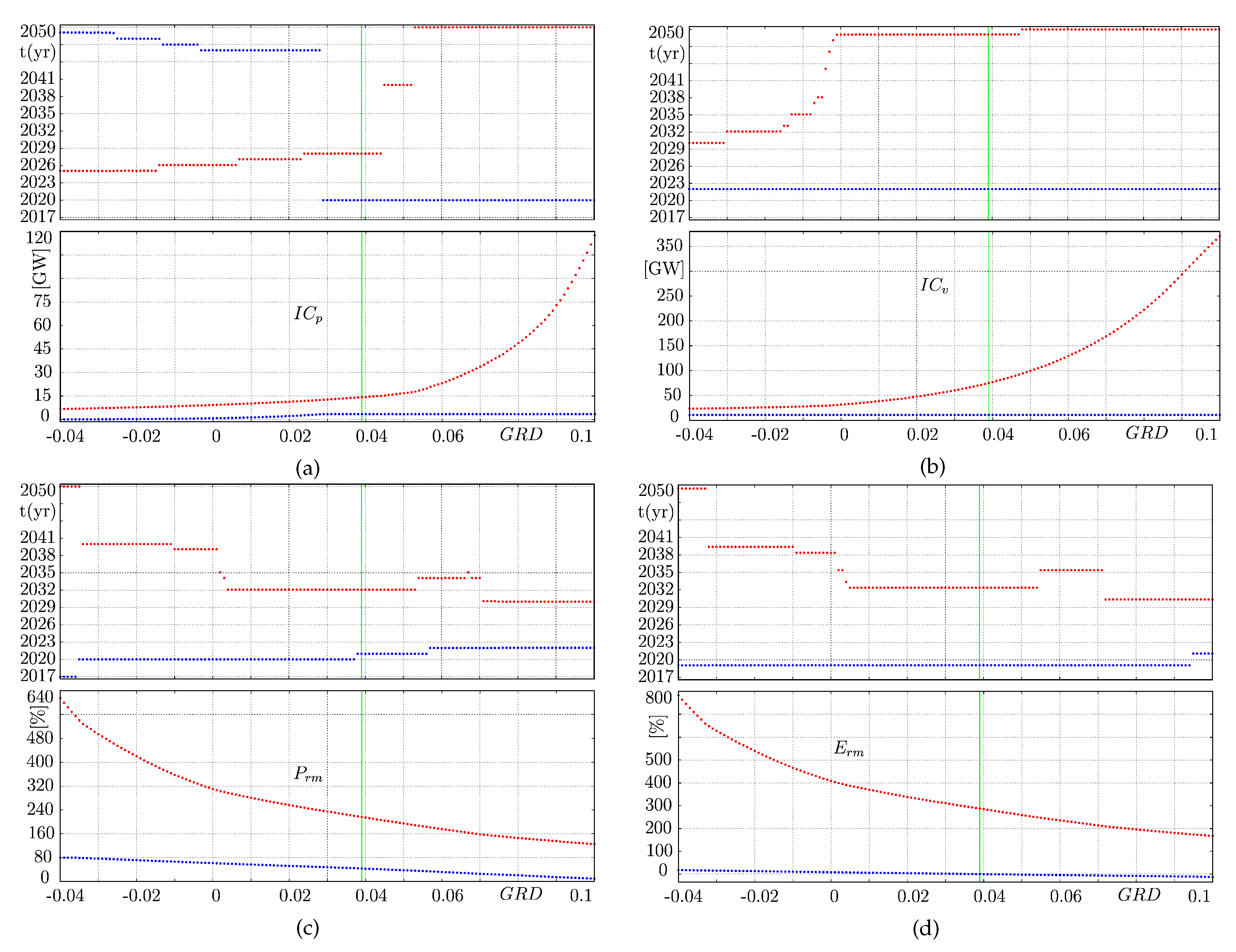
5.4. Confidence Limits and Their Occurrence

Advanced sensitivity diagrams based on bifurcation theory were obtained above to provide a deeper insight into the Colombian electricity market against $GRD$ variations and under variability imposed by seasonality and ENSO phenomenon. However, it is essential to investigate the confidence limits together with their time of occurrence. We applied DS tools to reach our goal and incentive this novel form of analysis for SD models that can extract more and complete information of possible scenarios.

As shown in Figure 12 and Figure 13, under the DS perspective, more information can be extracted from our SD model based on the bifurcation theory by illustrating the confidence limits together with their corresponding year of occurrence. In other words, the maximum and minimum values reached by the key market variables were plotted for each $GRD$ scenario.

As a first step, let us consider Figure 12a, which illustrates the confidence limits of $I{C}_p$ under different $GRD$ scenarios. Note that 50% of the $GRD$ scenarios (i.e., for negative $GRD$ values and some positive ones, up to 0.028) indicate that the permanent capacity tends to increase and gets a maximum value in the short or middle run, after which it starts to drop until it reaches a minimum value (close to 0 MW) in the long run, near 2045. Under negative and small positive values of $GRD$, the power market might expect to have a significant permanent capacity installed for 8–11 years. Then, after about 25 years, one can expect a considerable reduction in thermal capacity. However, if the $ed$ of Colombia is 0.029 ≤$GRD$≤ 0.044, Colombia might expect to have a significant reduction of its permanent share in the short run (2020) caused by its natural depreciation, but also a large increment of it in the middle term (2028) caused by the critical rationing events expected to occur in the short run, which then incentive the thermal capacity expansion. In fact, if the $ed$ of Colombia increases ($GRD$ > 0.045), the permanent capacity decreases in the short run, in 2020, but it might be necessary to incentivize a large increment of this capacity in the long run, about 2048, for supporting the variable renewable generation of such time. The $GRD$ scenarios together with the ENSO variability give us three possible energy prospects for thermal power generation. One of them (for $GRD$ < 0.029) suggests that the permanent capacity would continue to grow for at least 8 years, but it could disappear in the long term. The other one (0.029 ≤ $GRD$ ≤ 0.044) suggests that the permanent capacity tends to disappear in the short term, but it might become important in the middle term because of the new capacity investments conducted in previous years to overcome the critical situations encountered in the short run. In contrast, if the $GRD$ exceeds 0.045, it is very likely that the permanent capacity drops a lot in the near future but increases significantly in the long term to support the increasing variable renewable capacity.

Conversely, the behavior patterns of $I{C}_v$ (see Figure 12b) never drop significantly in the long run regardless of the $GRD$ scenario; its minimum value is always expected to occur around 2022 for the same reason explained above. Additionally, note that for −0.04 ≤ $GRD$ ≤−0.015, the maximum $I{C}_v$ is achieved close to 2030. Conversely, for −0.015 ≤ $GRD$ ≤ 0.1, the maximum $I{C}_v$ is normally achieved at the end of the simulation since the $ed$ is large enough to provoke critical values of $E_{rm}$ in prior years, which immediately incentivizes the investments in new hydropower capacity; however, the resulting increase in $I{C}_v$ occurs 5-years later (≈2049) because of issues associated with construction delays.

Furthermore, as shown in Figure 12c,d, $P_{rm}$ and $E_{rm}$ differ by a number of properties. In general terms, both $P_{rm}$ and $E_{rm}$ always exhibit their lowest values in the short run (around 2020) because of the natural depreciation of power plants, which is expected to significantly affect the margin level until the first new capacity is ready to operate. Additionally, our electricity market model is expected to attain the maximum $P_{rm}$ and $E_{rm}$ levels, principally, in the middle term and in the long term. It means that all power plants that are built to support the critical situations in the twenties give rise to a margin level overshoot a few years later. After that, both $P_{rm}$ and $E_{rm}$ start to drop again but do not reach a critical value in the long run.

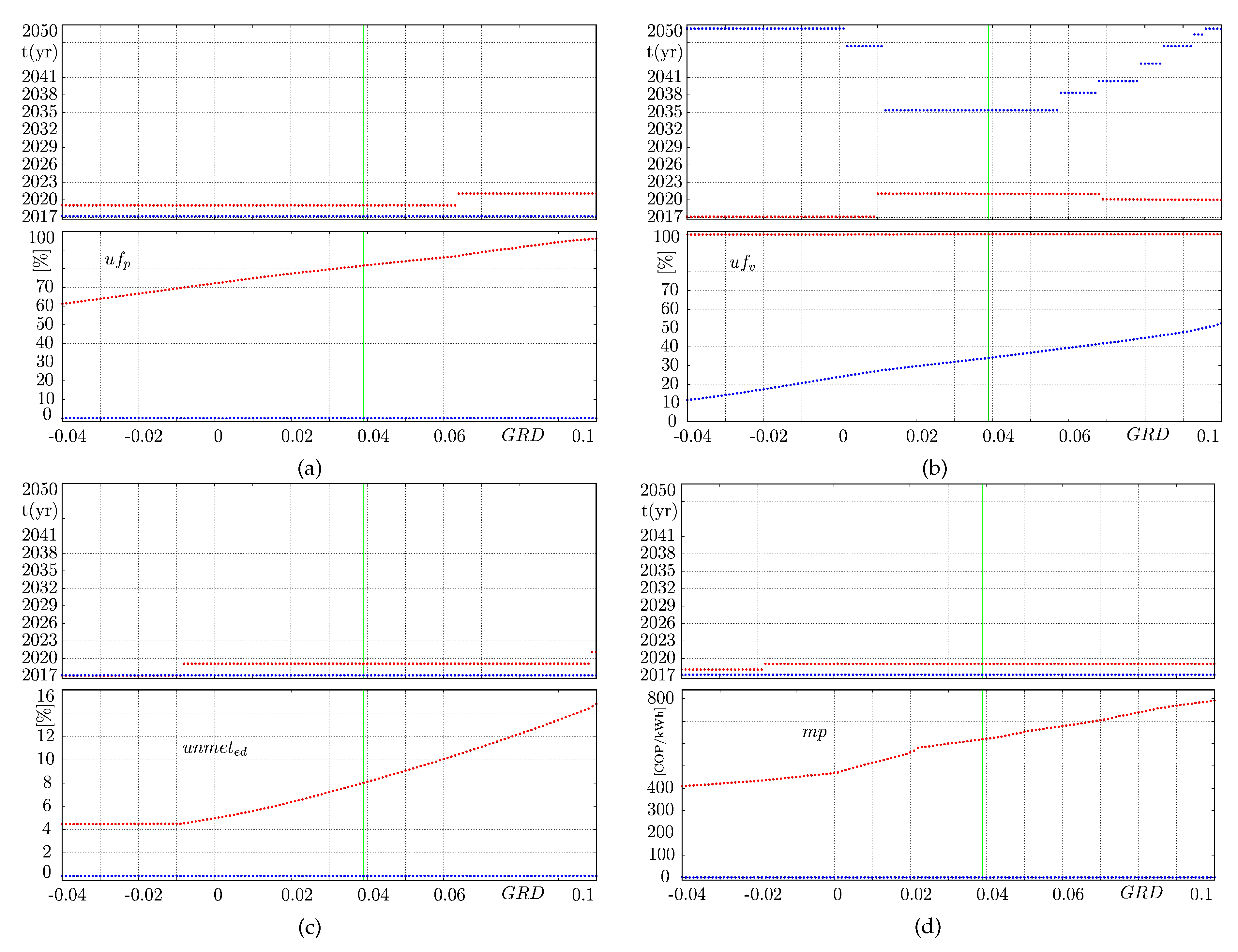
Moreover, Figure 13a,b illustrate the confidence limits of $u{f}_p$ and $u{f}_v$, respectively. $u{f}_p$ shows that the highest participation of thermal plants is basically required in the short run for all $GRD$ scenarios. Clearly, 2020–2021 can be cataloged as very critical years for the environment since almost the full potential of the fossil fuel power plants might be necessary to cover the total $ed$ regardless of the $GRD$ scenario. The lowest participation of thermal plants (Consequently, less CO${}_2$ emissions provided by fossil fuel generation) took place during 2019, once again regardless of the $GRD$ scenario. Thus, the ENSO phenomenon makes thermal power crucial for all $GRD$ scenarios to guarantee the security of supply, especially in the short run as the risks of blackouts persist.

Moreover, $u{f}_v$ shows that hydroelectricity plants participated with their full power in 2018, 2020, and 2021, indicating that the short run might be a very critical time for the Colombian power market if new and significant capacity is not installed prior to 2021. The worst cases for hydropower generation appear to be for negative and few positive $GRD$ scenarios and in the very long run; as shown, its participation goes from 12% to 25%. However, for most of the positive $GRD$ scenarios, the lowest participation of hydroelectricity plants (ranging from 25% to 52%) starts in the middle run because $P_{rm}$ and $E_{rm}$ have a safe value during this time. Clearly, as $GRD$ increases, the lowest participation of hydroelectricity plants becomes higher as well.

Finally, Figure 13c,d show $unme{t}_{ed}$ and $mp$, respectively. The ENSO phenomenon causes $unme{t}_{ed}$ episodes to appear for all $GRD$ values. For negative $GRD$, electricity rationing is much less than in other cases. Within the $GRD$ range (−0.04, −0.008), the worst $unme{t}_{ed}$ events occur in the very short run, whereas for $GRD$ (−0.007, 0.1), including the Colombian case, the worst $unme{t}_{ed}$ cases are expected to occur close to 2021. In fact, the exponential shape of $unme{t}_{ed}$ corresponds to rationing events taking place in a relatively further run (and no electricity rationing events appear in the long run), whereas the flat shape of $unme{t}_{ed}$ suggests rationing events appearing in the very short run but also fewer pronounced rationing events than the exponential one. Accordingly, it can be seen in Figure 13d that the $RAP$ is present in all $GRD$ scenarios and that the maximum $mp$ is reached close to 2021 regardless of the $GRD$ scenario, whereas the hydroelectricity price ($P_v$) is detected as the minimum price in the short run, once again regardless of the $GRD$ scenario. Although some rationing events appear and both thermal and hydropower plants dispatch electricity to meet the total $ed$, it is expected that $mp$ that consumers perceive are mostly set by thermal producers, as shown in Figure 9h.

As can be seen from Figure 12 and Figure 13, the policymakers can determine, for each market variable, the extreme conditions and when they are going to take place; this has never been constructed using SD models and has recently been introduced in [20].

5.5. Detailed Rationing Events: A Control Theory Pperspective

Now let us consider in more detail all the possible rationing events of the $GRD$ scenarios under the presence of the ENSO phenomenon in our model. As we discussed and showed above, all $GRD$ scenarios may exhibit $unme{t}_{ed}$ or rationing events if the ENSO phenomenon is incorporated in the model; therefore, here, we estimate the number of months expected to be under electricity rationing, their specific year, and even the exact month.

By using the input-output relationship diagram widely used in control theory through describing functions [40], we develop a graphical tool that can specifically determine how long rationing events are expected to undergo, their year and month of occurrence, and the probability of such episodes.

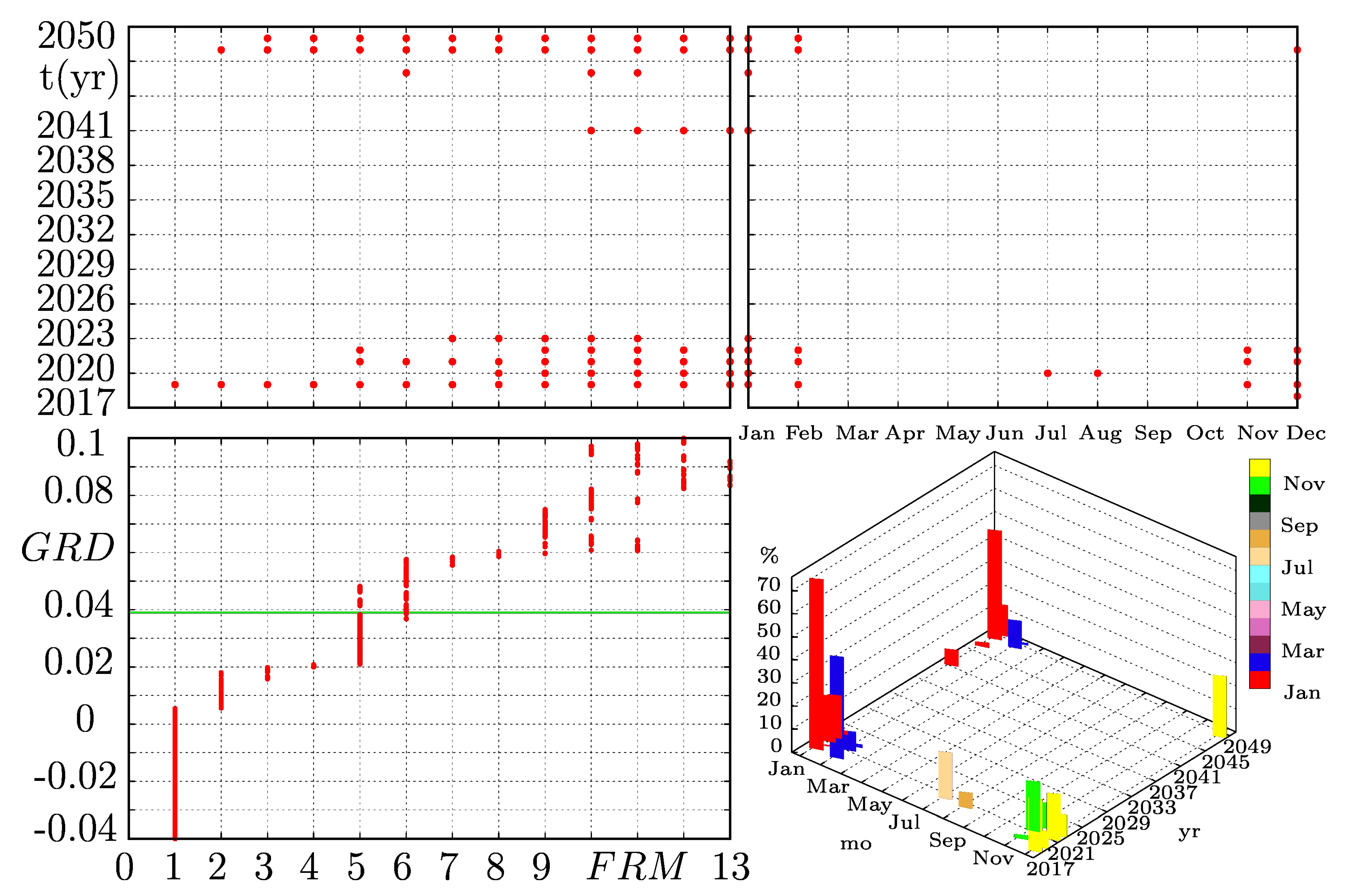
Figure 14 shows the input-output relationship diagram computed for every $GRD$ scenario; the bottom left diagram shows the $FRM$ (frequency of rationing months), the upper left and right diagrams illustrate their corresponding year and month of occurrence, and the bottom right diagram shows their corresponding probability of occurrence. In fact, our model undergoes different $FRM$ for each $GRD$ scenario; particularly, note that for $GRD$ values above 0.02, five or more months of electricity rationing are expected to occur during 2020–2023 and 2041–2050. According to the upper right diagram, these months might be mainly January, February, November, and December. However, January is prone to be the driest month of the year; hence, we infer January would most likely be the worst-case scenario for most of the $GRD$ values. Then, the 3-D diagram shows that January 2021 is one of the possible worst-case scenarios since it has a nearly 30% probability of occurrence. We conclude that if the $GRD$ reaches positive values, it is very likely that the power market undergoes an electricity crisis mainly in January in the short run and in the long run. Since Colombia went through a serious electricity shortage in 2019 due to the Hidroituango delay, which is also shown using our simulation model, the government should pay attention to the coming years to avoid unmet $ed$ events.

In more detail, Figure 14 shows that Colombia might undergo 5 months of electricity rationing. If we look at the mapped upper left diagram, it can be observed that these 5 months might take place in 2021, 2022, 2048, or 2049. However, it is possible to verify from the BaU Colombian scenario shown in Figure 9d, that events of $unme{t}_{ed}$ are expected to occur in 2022, 2048, and 2049. Accordingly, and looking very carefully to the $unme{t}_{ed}$ of the BaU scenario and at the corresponding mapped upper left diagram of Figure 14, we can conclude that Colombia might have 5 months of electricity rationing in 2021–2022, and 2048–2049 in January and February, July and August, and November and December. Finally, the bottom right 3-D diagram shows that January and February of 2021–2022 are some of the worst-case scenarios with probabilities of occurrence of 32% and 45%, respectively, which are followed by January of 2048 and 2049 with probabilities of occurrence of nearly 44% and 12%, respectively. Thus, officials must pay attention to mainly January 2021–2022 to avoid shortages. Our model shows that Colombia needs new power to be installed before 2022 to avoid probable rationing events.

The critical situations expected to happen in the short run can also incentive a safe period of time (from 2024 to 2040) in the middle run for the Colombian electricity market. These investments can be expected to provide sufficient power and competitive edge to the Colombian electricity market, if not in the short run, in the medium run (Figure 14).

6. Conclusions

The chaotic component intended to represent the variability of hydropower generation is highly transferred to $I{C}_p$ rather than $I{C}_v$ (which is the technology bringing variability to the system). This is basically explained by the dispatch merit order effect together with environmental and price issues. hydropower plants are built in accordance with the $ed$ growth, whereas thermal plants are built when hydroelectricity is not able to meet the total $ed$. However, since all the market variables are averaged, the chaotic components are not well pronounced.

Since the ENSO phenomenon onsets a stronger variability, $I{C}_p$ tends to develop its capacity. Generally, stronger variability influences more investments in permanent capacity to mitigate such variability. Therefore, less renewable capacity is installed. Indeed, we have validated with historical data that this conclusion has been present in the installation of permanent and variable capacity during the past decade.

Because of the nearly smooth growth of both $I{C}_p$ and $I{C}_v$, and the installation of a larger share of permanent generation as the $GRD$ varies, less variable $E_{rm}$ is achieved. Even though more permanent capacity is installed when the ENSO is part of the model, its variability leads $P_{rm}$ to critical instances for large $GRD$ values. In fact, even for the negative values of $GRD$, $E_{rm}$ reaches critical episodes and cannot avoid dropping to negative ones for larger $GRD$ values.

The ENSO phenomenon scenarios mainly show that variability, together with other issues, might provoke serious CO${}_2$ emission episodes in 2021–2022 since a very high potential of fossil fuel generation plants might be necessary to cover the total $ed$, regardless the $GRD$ scenario. This case has already been happening in Colombia because of the Hidroituango plant delay. Although there have not been unmet demand episodes, it caused a serious alert in the electricity system so that the government immediately called for a renewable auction in October 2019. Regardless of the $GRD$ scenario, the lowest participation of thermal plants (consequently, less CO${}_2$ emissions) is taking place nowadays during 2019.

Despite the chaotic variability of the ENSO phenomenon, certain patterns can be observed in the market variables with specific periods of time suffering from dry months, such as January, February, July, August, November, and December; the behavior patterns of the seasonality dominate the market dynamics, although the ENSO phenomenon chaotically disturbs its behavior.

Inspired by the control theory, the stock-flow structure of our proposed model was successfully and easily transformed into its equivalent block diagram of Simulink. Transforming the stock-flow structure in a block diagram of Simulink has shown to be the easiest way to have access to any DS tool. This transformation is very simple (as shown in [20,41]) and does not require mathematical equations. The same steps applied in Vensim, Stella, or Powersim to formulate the stock-flow structure can be applied in Simulink, just that some functions can change when using a different software package. In fact, irrespective of the level of abstraction or how big our model is, Simulink gives even more advantages than SD software. However, it is mandatory to construct the stock-flow structure in any SD software as usual, before resorting to Simulink.

Finally, further research will be developed to incorporate the import and export of electricity in our model and, in turn, explore how the Colombian power market might be affected by the ENSO phenomenon together with the import and export of electricity.

References

1. York, R.; Bell, S.E. Energy transitions or additions? Why a transition from fossil fuels requires more than the growth of renewable energy. Energy Res. Soc. Sci. 2019, 51, 40–43. [Google Scholar] [CrossRef]
2. Ebhota, W.S.; Jen, T.C. Fossil Fuels Environmental Challenges and the Role of Solar Photovoltaic Technology Advances in Fast Tracking Hybrid Renewable Energy System. Int. J. Precis. Eng. Manuf. Green Technol. 2019, 7, 97–117. [Google Scholar] [CrossRef]
3. Ray, M.; Chakraborty, B. Impact of evolving technology on collaborative energy access scaling. Renew. Sustain. Energy Rev. 2019, 110, 13–27. [Google Scholar] [CrossRef]
4. Agency, I.E. Variability of Wind Power and Other Renewables: Management Options and Strategies; International Energy Agency: Paris, France, 2005. [Google Scholar]
5. Dagoumas, A.S.; Koltsaklis, N.E. Review of models for integrating renewable energy in the generation expansion planning. Appl. Energy 2019, 242, 1573–1587. [Google Scholar] [CrossRef]
6. Odeh, R.P.; Watts, D. Impacts of wind and solar spatial diversification on its market value: A case study of the Chilean electricity market. Renew. Sustain. Energy Rev. 2019, 111, 442–461. [Google Scholar] [CrossRef]
7. Ren, S.; Dou, X.; Wang, Z.; Wang, J.; Wang, X. Medium-and Long-Term Integrated Demand Response of Integrated Energy System Based on System Dynamics. Energies 2020, 13, 710. [Google Scholar] [CrossRef] [Green Version]
8. Teufel, F.; Miller, M.; Genoese, M.; Fichtner, W. Review of System Dynamics Models for Electricity Market Simulations; Working Paper Series in Production and Energy; KIT: Karlsruhe, Germany, 2013. [Google Scholar]
9. Pillay, N.S.; Brent, A.C.; Musango, J.K.; van Geems, F. Using a System Dynamics Modelling Process to Determine the Impact of eCar, eBus and eTruck Market Penetration on Carbon Emissions in South Africa. Energies 2020, 13, 575. [Google Scholar] [CrossRef] [Green Version]
10. Rebs, T.; Brandenburg, M.; Seuring, S. System dynamics modeling for sustainable supply chain management: A literature review and systems thinking approach. J. Clean. Prod. 2019, 208, 1265–1280. [Google Scholar] [CrossRef]
11. Zapata, S.; Castaneda, M.; Franco, C.J.; Dyner, I. Clean and secure power supply: A system dynamics based appraisal. Energy Policy 2019, 131, 9–21. [Google Scholar] [CrossRef]
12. Sterman, J.D. Business Dynamics: Systems Thinking and Modeling for a Complex World; Irwin/McGraw-Hill: New York, NY, USA, 2000; p. 1008. [Google Scholar] [CrossRef]
13. Mao, G.; Dai, X.; Wang, Y.; Guo, J.; Cheng, X.; Fang, D.; Song, X.; He, Y.; Zhao, P. Reducing carbon emissions in China: Industrial structural upgrade based on system dynamics. Energy Strategy Rev. 2013, 2, 199–204. [Google Scholar] [CrossRef]
14. González, M.; González, F.; Luaces, A.; Cuadrado, J. A collaborative benchmarking framework for multibody system dynamics. Eng. Comput. 2010, 26, 1–9. [Google Scholar] [CrossRef]
15. Aracil, J. Structural stability of low-order system dynamics models. Int. J. Syst. Sci. 1981, 12, 423–441. [Google Scholar] [CrossRef]
16. Mosekilde, E.; Aracil, J.; Allen, P.M. Instabilities and chaos in nonlinear dynamic systems. Syst. Dyn. Rev. 1988, 4, 14–55. [Google Scholar] [CrossRef]
17. Thomsen, J.S.; Mosekilde, E.; Sterman, J.D. Hyperchaotic phenomena in dynamic decision making. In Complexity, Chaos, and Biological Evolution; Springer: Berlin/Heidelberg, Germany, 1991; pp. 397–420. [Google Scholar]
18. Aracil, J. On the qualitative properties in system dynamics models. Eur. J. Econ. Soc. Syst. 1999, 13, 1–18. [Google Scholar] [CrossRef]
19. Redondo, J.M.; Olivar, G.; Ibarra-Vega, D.; Dyner, I. Modeling for the regional integration of electricity markets. Energy Sustain. Dev. 2018, 43, 100–113. [Google Scholar] [CrossRef]
20. Morcillo, J.D.; Franco, C.J.; Angulo, F. Simulation of demand growth scenarios in the Colombian electricity market: An integration of system dynamics and dynamic systems. Appl. Energy 2018, 216, 504–520. [Google Scholar] [CrossRef]
21. Jaramillo, G.P. Atractores extraños (caos) en la hidro-climatología de Colombia? Rev. Acad. Colomb. Cienc. 1997, 21, 431–444. [Google Scholar]
22. Tziperman, E.; Stone, L.; Cane, M.A.; Jarosh, H. El Niño Chaos: Overlapping of Resonances Between the Seasonal Cycle and the Pacific Ocean-Atmosphere Oscillator. Science 1994, 264, 72–74. [Google Scholar] [CrossRef] [Green Version]
23. XM. Oferta y Generación. Índice Multivariado ENSO. 2013. Available online: http://informesanuales.xm.com.co/2013/SitePages/operacion/2-9-Anex-Indice-multivariado-ENSO.aspx (accessed on 10 January 2017).
24. XM. Portal BI: Información Inteligente. 2018. Available online: http://informacioninteligente10.xm.com.co/hidrologia/Paginas/HistoricoHidrologia.aspx (accessed on 10 January 2018).
25. Margarita, M.; Zárate, T.; Hernández, V.A. Colombia Energy Investment Report. Electronic, International Energy Chapter. 2016. Available online: http://www.energycharter.org/what-we-do/publications/colombia-energy-investment-report/ (accessed on 6 April 2020).
26. Dyner, I. Energy modelling platforms for policy and strategy support. J. Oper. Res. Soc. 2000, 51, 136–144. [Google Scholar] [CrossRef]
27. Morcillo, J.D.; Franco, C.J.; Angulo, F. Delays in electricity market models. Energy Strategy Rev. 2017, 16, 24–32. [Google Scholar] [CrossRef]
28. Espinosa, O.; Vaca, P.; Ávila, R. Elasticidades de demanda por electricidad e impactos macroeconómicos del precio de la energía eléctrica en Colombia. Revista de Métodos Cuantitativos para la Economía y la Empresa 2013, 16, 216–249. [Google Scholar]
29. Nelson, D.C. A Study of the Elasticity of Demand for Electricity by Residential Consumers: Sample Markets in Nebraska. Land Econ. 1965, 41, 92–96. [Google Scholar] [CrossRef]
30. Weitzman, M.L. Prices vs. quantities. Rev. Econ. Stud. 1974, 41, 477–491. [Google Scholar] [CrossRef]
31. Siddiqui, A.S. Price Elastic Demand in Deregulated Electricity Markets; Technical Report; LBNL: Berkeley, CA, USA, 2003. [Google Scholar]
32. Bernstein, M.A.; Griffin, J. Regional Differences in the Price-Elasticity of Demand for Energy; Technical Report; National Renewable Energy Lab. (NREL): Golden, CO, USA, 2006. [Google Scholar]
33. Slingo, J.; Palmer, T. Uncertainty in weather and climate prediction. Philos. Trans. R. Soc. Lond. A Math. Phys. Eng. Sci. 2011, 369, 4751–4767. [Google Scholar] [CrossRef]
34. Barlas, Y. Formal aspects of model validity and validation in system dynamics. Syst. Dyn. Rev. 1996, 12, 183–210. [Google Scholar] [CrossRef]
35. Qudrat-Ullah, H.; Seong, B.S. How to do structural validity of a system dynamics type simulation model: The case of an energy policy model. Energy Policy 2010, 38, 2216–2224. [Google Scholar] [CrossRef]
36. EPM. Proyecto Hidroeléctrico Ituango. 2019. Available online: https://www.epm.com.co/site/nuestros-proyectos/proyecto-ituango (accessed on 14 December 2019).
37. EPM. Especial Contingencia HidroItuango. 2019. Available online: https://www.epm.com.co/site/home/camino-al-barrio/historias-de-barrio/especial-hidroituango-1 (accessed on 14 December 2019).
38. XM. XM Presenta Análisis de Posibles Escenarios para la Atención de la Demanda Eléctrica del País. 2018. Available online: https://www.xm.com.co/Paginas/detalle-noticias.aspx?identificador=1747 (accessed on 10 December 2019).
39. Valencia, J.; Franco, C.J.; Olivar, G.; Dyner, I. Enfoque metodológico para el estudio y representación de comportamientos complejos en mercados de electricidad. Ing. Cienc. 2016, 12, 195–220. [Google Scholar] [CrossRef] [Green Version]
40. Vander Velde, W.E. Multiple-Input Describing Functions and Nonlinear System Design; McGraw-Hill: New York, NY, USA, 1968. [Google Scholar]
41. Dimitrovski, A.; Ford, A.; Tomsovic, K. An interdisciplinary approach to long-term modelling for power system expansion. Int. J. Crit. Infrastruct. 2006, 3, 235–264. [Google Scholar] [CrossRef]
Figure 1. Dynamic hypothesis derived from [26].
Energies 13 02381 g001
Figure 2. Electricity supply from (P) generation.
Energies 13 02381 g002
Figure 3. Electricity supply from (V) generation.
Energies 13 02381 g003
Figure 4. Demand component.
Energies 13 02381 g004
Figure 5. Electricity dispatch.
Energies 13 02381 g005
Figure 6. a f v . The red signal represents the real behavior of the aggregate flow series of Colombian rivers obtained from [24]. The blue signal is computed by the author using Equations (1) and (2). The MAPE (mean absolute percentage error) = 11.35 %.
Energies 13 02381 g006
Figure 7. SD modeling of the ENSO phenomenon. Stock-flow structure of a f v .
Energies 13 02381 g007
Figure 8. The DS modeling approach of the ENSO phenomenon. Simulink block diagram of a f v .
Energies 13 02381 g008
Figure 9. Simulation of the Colombian electricity market under seasonality and ENSO, considering the BaU scenario. (a) Capacity under construction (P) - C u C p and capacity under Construction (V) - C u C v , (b) installed capacity (P) - I C p and installed capacity (V) - I C v , (c) electricity demand - e d , dispatch (P) - d i s p p and dispatch (V) - d i s p v , (d) unmet e d - u n m e t e d , (e) power reserve margin - P r m , (f) energy reserve margin - E r m , (g) utilization factor (P) - u f p and utilization factor (V) - u f v , and (h) market price - m p .
Energies 13 02381 g009
Figure 10. Variance of the u n m e t e d (Var( u n m e t e d )) computed for 6000 simulations. Each simulation was obtained from a different initial condition of z ( z ( 0 ) ).
Energies 13 02381 g010
Figure 11. G R D scenarios under seasonality and ENSO phenomenon. G R D was varied from −0.04 to 0.1. The green rectangles marked in all figures represent the current Colombian scenario ( G R D = 0.039) (a) I C p , (b) I C v , (c) P r m , (d) E r m , (e) u f p , (f) u f v , (g) u n m e t e d , and (h) m p .
Energies 13 02381 g011
Figure 12. Confidence limits of the G R D scenarios together with their time of occurrence, when seasonality and ENSO phenomenon are considered. The marked green vertical line represents the Colombian case ( G R D = 0.039) (a) I C p , (b) I C v , (c) P r m , and (d) E r m .
Energies 13 02381 g012
Figure 13. Confidence limits of the G R D scenarios together with the time of occurrence, under seasonality and ENSO phenomenon. The marked green vertical line represents the Colombian case ( G R D = 0.039) (a) u f p , (b) u f v , (c) u n m e t e d , and (d) m p .
Energies 13 02381 g013
Figure 14. Diagram of the G R D scenarios once the ENSO phenomenon is incorporated in the model. F R M stands for frequency of rationing months. The Colombian case is marked by the green horizontal line.
Energies 13 02381 g014