Two-Dimensional Tomographic Simultaneous Multispecies Visualization—Part II: Reconstruction Accuracy

Abstract

Recently we demonstrated the simultaneous detection of the chemiluminescence of the radicals OH* (310 nm) and CH* (430 nm), as well as the thermal radiation of soot in laminar and turbulent methane/air diffusion flames. As expected, a strong spatial and temporal coupling of OH* and CH* in laminar and moderate turbulent flames was observed. Taking advantage of this coupling, multispecies tomography enables us to quantify the reconstruction quality completely independent of any phantom studies by simply utilizing the reconstructed distribution of both species. This is especially important in turbulent flames, where it is difficult to separate measurement noise from turbulent fluctuations. It is shown that reconstruction methods based on Tikhonov regularization should be preferred over the widely used algebraic reconstruction technique (ART) and multiplicative algebraic reconstruction techniques (MART), especially for high-speed imaging or generally in the limit of low signal-to-noise ratio.

1. Introduction

Optical emission tomography facilitates the detection of 2D or even 3D distributions of the chemiluminescence emission of laminar and turbulent hydrocarbon flames of any geometry. The development and application of tomographic methods for the reconstruction of flame structures in laminar and turbulent flames have gained a lot of interest in the past decade [1,2], for example, to image the distribution of chemiluminescent species [3,4,5,6,7,8,9,10,11,12,13,14,15,16,17,18,19,20,21,22,23,24,25,26,27,28,29] or the volumetric OH-LIF signal [30,31,32,33], as well as the 3D flow field using tomographic particle image velocimetry (tomo PIV) [2,34,35,36,37]. Floyd et al. [6] and Anikin et al. [3] were the first to investigate turbulent flames with optical emission tomography. More recently the focus has shifted towards space- and time-resolved tomographic measurements with kHz-repetition rate [8,13,15,17,25,28,29,31].

The quality and reliability of tomographic reconstruction methods applied to turbulent flames has hitherto been assessed solely on the basis of numerical studies on phantoms, see for example [4,6,7,15,38,39,40]. In these studies, the radon projections are simulated based on a model distribution, and the reconstructed distribution is compared with the model distribution as a function of noise level. So far it was the only viable method, because there is no ground-truth to objectively and independently judge the reconstruction quality of experimental data. This is particularly problematic in the reconstruction of turbulent flow fields, where an objective evaluation of the noise level (measurement error) in the projection data is nearly impossible and raises criticism as to whether the reconstructed structures are real or dominated by reconstruction artifacts. In order to be able to assess the quality of the reconstruction, a reliable knowledge of the actual signal-to-noise ratio in the turbulent flow field is essential. This also applies to phantom studies if they are used for validation. Here, multi-wavelength detection [41] opens a new tool by exploiting the strong spatial and temporal coupling of OH* and CH* [42,43,44,45,46] and the independence of the detection noise at both wavelengths. The last point is crucial in this context: while both species are subject to the same turbulent fluctuations, the photon and detector noise is statistically in its nature and therefore independent of each other at both wavelengths.

In our previous work (Part I [41]), we presented a novel extension (${\mathrm{POET}}^{\lambda })$ of our planar emission tomograph ($\mathrm{POET}$) that enables the simultaneous detection of multiple wavelengths or species in laminar and turbulent flames using a single image-intensified camera. In this work (Part II) we will take advantage of the strong spatial and temporal coupling of OH* and CH* in laminar and moderate turbulent flames to quantify the reconstruction quality completely independent of any phantom studies. We will show that the spatial location of turbulent flame fronts can indeed be reproduced with high probability. However, reconstruction methods based on Tikhonov regularization [40,47,48] should be preferred over the widely used algebraic reconstruction technique (ART) [49,50] and multiplicative algebraic reconstruction techniques (MART) [49,51,52,53], especially for high-speed imaging of turbulent flames or generally in the limit of low signal-to-noise ratio. We will also show that the validation of tomographic methods based on the back projection of reconstructed distributions, as recently suggested in the literature [12,13,15,28,29], is flawed. The good agreement between experimental and back-projected data is a necessary but not a sufficient condition for the quality of the reconstruction.

2. Materials and Methods

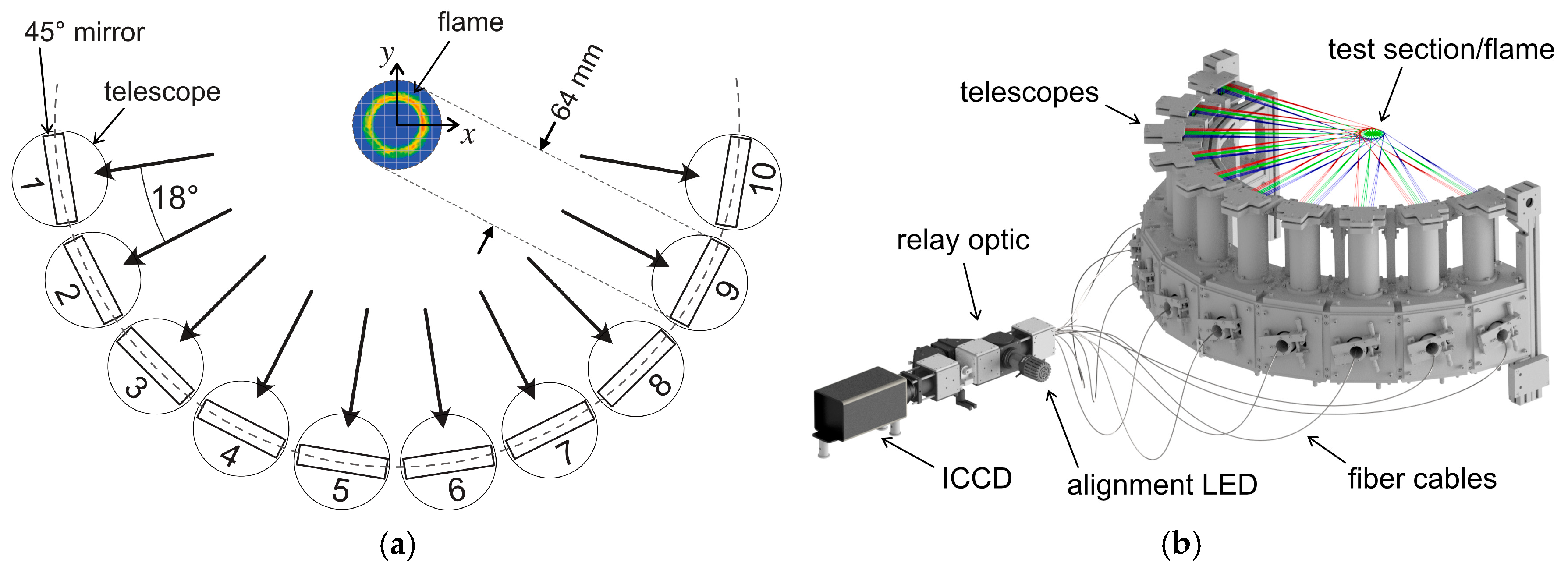
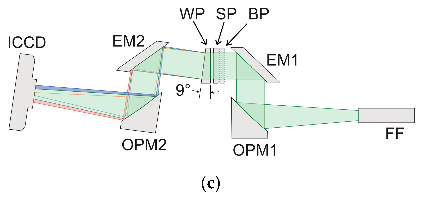
2.1. Tomographic Setup

The tomographic setup has been described in detail previously [41]. Briefly, it consists of ten telescopes arranged in a semicircle around the flame, as shown in Figure 1. The flame emission is deflected into the vertical direction by UV-enhanced $45$° aluminum mirrors mounted on top of each telescope, which projects the light onto a row of optical fibers. The telescopes perform two important functions: (1) They ensure that each optical fiber detects the luminescence signal only at a small solid angle in space and (2) they map the field of view ($64$ mm) to the length of a fiber row, with a reduction factor of $5.7$. All ten fiber rows are bundled into a single ferrule and the emitted light is imaged onto a single intensified charged coupled device camera (ICCD, PIMAX 4, Princeton Instruments). Each leg of the fiber bundle (Ceram Optec SIA) contains 102 fused silica fibers (NA $0.22$, core ⌀$100$ µm, outer ⌀$125$µm, including polyimide jacket) densely packed and arranged side by side in a row. On the telescope side the polyimide jacket has been removed from the fibers to allow for a denser packing of the bare fibers (⌀$110$µm) and, hence, a better optical resolution with a total length of each fiber row of $11.22$ mm ($102\times 110$ µm).

Towards the camera, the optical fibers are brought together in a single ferrule in which the individual fiber rows of the different telescopes are stacked one above the other, each separated by a stainless-steel spacer. The output signal of the optical fibers is collimated by an off-axis parabolic mirror (OPM1) and deflected by a flat elliptical mirror (EM1) through a short-pass filter (SP) and a wedged prism (WP), as displayed in Figure 1c. The signal of each individual optical fiber is spatially separated into its wavelengths by the prism and imaged through another set of mirrors (EM2 & OPM2) onto the image-intensified CCD camera (ICCD). The short-pass (SP) filter prevents crosstalk of the spectrally separated signals from neighboring rows of optical fibers. Optionally, a band-pass filter (BP) can be used to limit the detection wavelength to a specific species, e.g., OH* @ 308 nm or CH* @ 431 nm. The reconstruction grid consists of $102\times 102$ grid cells and the tomographic setup has an effective optical resolution in the tomographic measurement plane of about $2$ cells or $\sim 1.3$ mm, in accordance with the Nyquist–Shannon sampling theorem [41]. Perpendicular to the measurement plane the optical resolution is $0.9\pm 0.3$ mm.

In the following, the coordinate system is defined as (compare Figure 1a): The coordinate system is centered in the middle of the flame or the measurement region, with the $z$-axis (vertical direction) oriented perpendicular to the measurement plane. The acute angle between the $x$-axis and the projection directions of telescopes 1 and 10 is $9°$. The $y$-axis lies in the middle between projection directions 5 and 6.

2.2. Tomographic Reconstruction

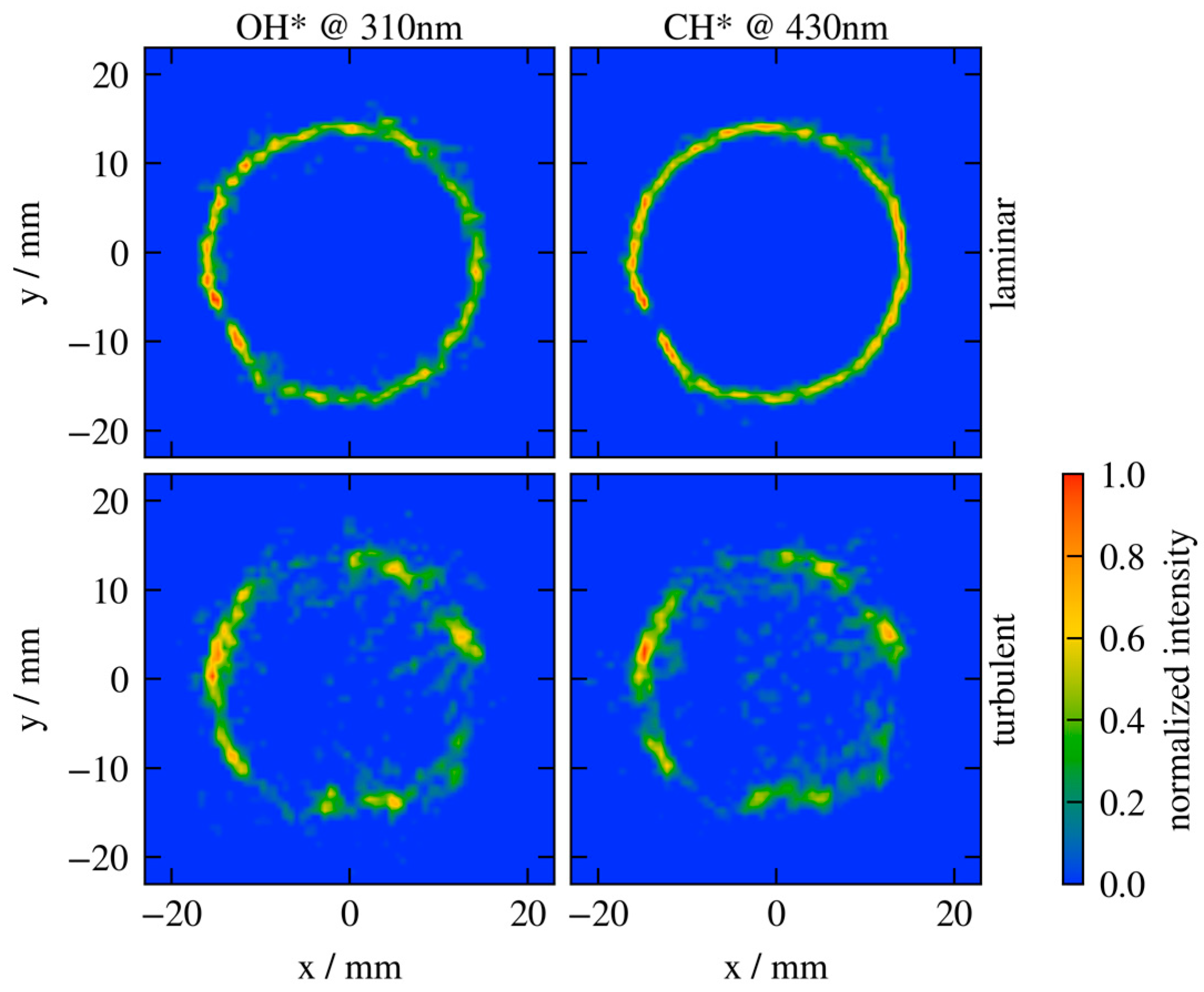
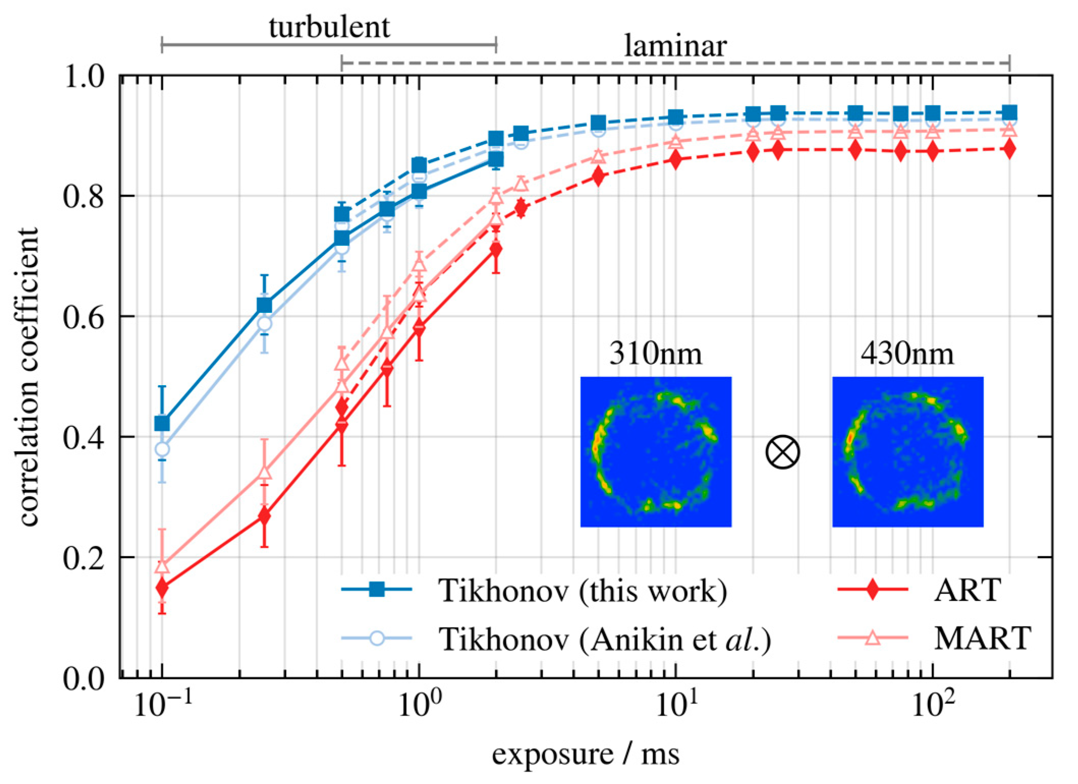
For the reconstruction, the measurement area is divided into a Cartesian grid with $n=102\times 102$ elements and an edge length of $64$ mm. In the following, we assume that the flame is a low scattering optical medium with homogeneous refractive index even for sooting flames, so that the light follows a straight line from the emission source in the flame to the detector. That is, index gradients caused by fluctuations of the local flame temperature and species concentrations are neglected. Under this assumption, each projection $b_i$ can be approximated as a “ray-sum” [4,40,54]:

$$b_i={\displaystyle \sum }_j^n{A}_{ij}{x}_j$$

(1)

here $x_j$ is the unknown species concentration at pixel $j$ and $A_{ij}$ is the contribution of pixel $j$ to the projection $i$. Reconstructing the species distribution from the set of $m=10\times 102$ projections then requires solving a set of linear equations,

$$\mathit{A}\mathit{x}=\mathit{b}$$

(2)

where $\mathit{b}\in {ℝ}^m$ is a vector containing the measured projection intensities and $\mathit{x}\in {ℝ}^n$ are the unknown species concentrations. Since we are in the limit of low optical density and low optical scattering, the projection matrix $\mathit{A}\in {ℝ}^{m\times n}$ is constant, specific to the selected arrangement and only needs to be determined once. However, one cannot solve for the species concentrations directly, because the linear system is not well-posed, as defined by Hadamard [55]. More specifically, Equation (2) is rank-deficient, meaning that it permits an infinite number of solutions and additional assumptions must be made to limit the solution space [40,48]. Additionally, the solution does not depend continuously on the measured projections. Small changes (errors) of the projection data caused, e.g., by noise, are amplified and lead to extreme changes in the solution vector $\mathit{x}$. Both problems can be mitigated by regularization methods [40,47,48,54]. In this work, we use a combination [56,57] of 1st order Tikhonov regularization [47] and compressive sensing [58]. The species concentration is then obtained by solving the optimization problem:

$$\begin{array}{l}\hspace{1em}\hspace{1em}\hspace{1em}\hspace{1em}\hspace{1em}\hspace{1em}\hspace{1em}\hspace{1em}\mathit{x}=\arg \min \left[f\left(\mathit{x}\right)\right]\hspace{1em}\hspace{1em}\hspace{1em}\hspace{1em}\hspace{1em}\hspace{1em}\hspace{1em}\hspace{1em}\hspace{1em}\hspace{1em}\mathrm{s}.\mathrm{t}. \mathit{x}\ge 0\\ \mathrm{with}\\ \hspace{1em}\hspace{1em}\hspace{1em}\hspace{1em}f\left(\mathit{x}\right)={\Vert \mathit{A}\mathit{x}-\mathit{b}\Vert }_2^2+{\lambda }_1{\Vert \mathit{L}\mathit{x}\Vert }_2^2+{\lambda }_2{\Vert \mathit{x}\Vert }_1^2\\ \mathrm{and} {\Vert \dots \Vert }_q≔{\left({\sum }_j{\left|x_j\right|}^q\right)}^{1/q} \mathrm{and} L_{ij}=\{\begin{array}{cc}1& i=j\\ -1/n_i& i neighboring j\\ 0& otherwise\end{array}\end{array}$$

(3)

here ${\Vert \dots \Vert }_q$ denotes the Euclidian norm ($q=2$) or Manhatten norm ($q=1$). $n_i$ is the number of direct neighbors to pixel $i$, apart from the edges of the reconstruction grid, $n_i=4$. The Laplacian $\mathit{L}$ adds an additional set of $n$ equations to the linear system to remedy the rank-deficiency and enforces a piecewise smooth distribution. The extra term, ${\lambda }_2{\Vert \mathit{x}\Vert }_1^2$, has its origin in compressive sensing theory and minimizes the number of nonzero pixels [58]. Practically, it enforces the species concentrations to be zero in areas where the signal is close to or below the noise level. In statistics and machine learning, Tikhonov regularization and compressive sensing are also known as ridge and lasso regression, respectively. Since the classical L-curve method is not recommended for determining the optimal regularization parameters for the specified regularization scheme used here [40,59], the optimal parameters were determined by trial-and-error and phantom studies. Basically, the reconstruction was tested with different parameters and a combination was chosen in which the distribution is not excessively smeared by the regularization. The reconstruction of experimental distributions and the phantom studies share the same parameters. Although, this is not a robust method for determining ${\lambda }_1$ and ${\lambda }_2$, any analytical or quantitative method would only improve the reconstruction result compared to our values, especially for the phantom studies in Section 3. Equation (3) is solved by a gradient descent solver until the scalar objective function values of two successive iteration steps fulfill the convergence criterion:

$${ϵ}_1=\frac{f^{\left(p\right)}-f^{\left(p-1\right)}}{\max \left(f^{\left(p\right)},f^{\left(p-1\right)}\right)}<{10}^{-6}$$

(4)

where $f^{\left(p\right)}=f\left({\mathit{x}}^{\left(p\right)}\right)$ is the scalar objective function value in the $p$-th iteration. The convergence threshold has been set to a sufficiently low value, such that we do not observe any significant improvement (change) in the reconstructed distribution upon further tightening the convergence criterion. Its choice is validated by the phantom studies in Section 3.

For comparison, we will also include and apply the 0th-order Tikhonov regularization from our previous work [3,4]. In that case, the regularization term just consists of the Euclidian norm of the target distribution, without the Laplace operator, and the optimization problem simplifies to:

$$\mathit{x}=\arg \min \left[{\Vert \mathit{A}\mathit{x}-\mathit{b}\Vert }_2^2+\lambda {\Vert \mathit{x}\Vert }_2^2\right]\hspace{1em}\hspace{1em}\hspace{1em}\mathrm{s}.\mathrm{t}. \mathit{x}\ge 0$$

(5)

To the best of our knowledge, the work of Anikin et al. [3,4] is so far the only study that uses Tikhonov regularization for the tomographic imaging of laminar and turbulent flames. The vast majority of tomographic studies on combustion processes uses either the algebraic reconstruction technique (ART) [6,7,10,11,12,13,14,15,16,17,19,20,23,28,29,60] or its sibling, the multiplicative algebraic reconstruction technique (MART) [21,22,25,26,30,31,32]. ART was developed independently by Gordon, Bender and Herman [49] and Hounsfield [50]. It is based on an iterative process developed by Kacmarz [61] for solving consistent, linear systems of equations. The original ART algorithm is characterized by a rapid convergence with regard to the sum of squared errors, but shows a pronounced salt-and-pepper noise in the reconstructed distributions. Various variants have been developed to suppress noise artifacts and to improve convergence [34,51,52,62,63]. However, ART is used in its original formulation in almost all tomographic investigations of flames:

$$\begin{array}{lll}\mathrm{ART}:& \hspace{1em}\hspace{1em}{x}_j^{\left(p+1\right)}=x_j^{\left(p\right)}+{\omega }_j\left(b_i-{\displaystyle \sum _k^n}{A}_{ik}{x}_k^{\left(p\right)}\right)& \hspace{1em}\hspace{1em}\hspace{1em}\hspace{1em}\mathrm{s}.\mathrm{t}. x_j\ge 0\\ & \hspace{1em}\hspace{1em}\hspace{1em}\mathrm{with} {\omega }_j=\frac{\beta A_{ij}}{{\sum }_k^n{A}_{ik}^2}& \begin{array}{c}\hspace{1em}\hspace{1em}j=1\dots n\wedge i=1\dots m\\ p=1, 2,\dots \end{array}\end{array}$$

(6)

here $x_j^{\left(p\right)}$ is the solution at pixel $j$ in the $p$-th iteration and $\beta <1$ a relaxation factor, which controls the speed of convergence. Just like with Tikhonov regularization, the solution is limited to positive values. This constraint is implicit in many publications but is not always explicitly mentioned.

In many cases, particularly for tomographic particle imaging velocimetry (tomo-PIV) [2,34,35,36,37], MART is preferred over ART because of its faster convergence, while maintaining similar performance in terms of reconstruction accuracy [49,51,52,53]. In MART the solution is updated in each iteration step in a multiplicative fashion:

$$\begin{array}{ccc}\mathrm{MART}:& x_j^{\left(p+1\right)}=x_j^{\left(p\right)}{\left(\frac{b_i}{{\sum }_k^n{A}_{ik}{x}_k^{\left(p\right)}}\right)}^{\beta A_{ij}}& \begin{array}{c}\mathrm{s}.\mathrm{t}. x_j\ge 0\\ j=1\dots n\wedge i=1\dots m\\ p=1, 2,\dots \end{array}\end{array}$$

(7)

Unlike ART, the exact solution obtained with MART depends on the initial distribution. Conceptually, ART finds the solution with minimal energy, while MART maximizes the entropy of the reconstructed image if and only if the initial solution is uniform [53]. Without measures to terminate the iterative process prematurely, however, both methods eventually approach a solution that approximates the least squares solution to Equation (2). This is desirable in the case of discrete ill-posed problems, but is problematic when using these methods to solve rank-deficient problems. We will discuss this point and the impact of termination criteria in more detail later in the text.

Unless otherwise stated, we will use the normalized difference between the Euclidian norm of the solution vectors of two successive iteration steps as the termination criterion for ART and MART:

$${ϵ}_2=\frac{\left|{\Vert {\mathit{x}}^{\left(p\right)}\Vert }_2-{\Vert {\mathit{x}}^{\left(p-1\right)}\Vert }_2\right|}{{\Vert {\mathit{x}}^{\left(p\right)}\Vert }_2}<{10}^{-4}\cdot \beta$$

(8)

with $\beta =0.1$ and $0.01$ for ART and MART, respectively. The termination criterion is similar to that defined in [6,38,64,65]. However, there is still a large number of papers that do not provide any information on the exact termination criterion, which makes it difficult to assess the results.

3. Results

One of the key innovations of the new tomographic setup is the ability to detect multiple wavelengths, and thus different species simultaneously [41]. Figure 2 shows typical, simultaneously measured distributions of OH* and CH* of laminar (top) and turbulent (bottom) methane–air flames $5$ mm and $13.3$ mm above the burner, respectively. The exposure time in all cases is $1$ ms and each distribution is normalized by its maximum value. OH* and CH* are commonly used as flame front markers because their spatial location is inherently tied to the position of maximum heat release rate, even in turbulent flames [42]. The relative location between the maximum heat release rate and that of OH* or CH* changes only slightly with the strain rate and curvature of the flame front [42]. The same applies to the ratio of the chemiluminescence intensities, at least under moderately turbulent conditions [42,66,67]. In addition, since the luminescence lifetime of OH* and CH* is only about $1$ ns [68], there is no appreciable interaction between the electronically excited species and the turbulent flow field. Thus, we expect a strong correlation between OH* and CH* in space and time.

A very good spatial overlap of the measured OH* and CH* distributions can already be observed visually in Figure 2. This is quantitatively expressed by the normalized correlation coefficient [69] between the two distributions:

$$\begin{array}{cc}\rho \left(\mathit{x},\mathit{y}\right)=\frac{{\sum }_i\left(x_i-\overline{x}\right)\left(y_i-\overline{y}\right)}{s_x{s}_y}& \hspace{1em}\hspace{1em}\hspace{1em}i=1\dots n\end{array}$$

(9)

where $\overline{x}$ and $\overline{y}$ are the mean values and $s_x$ and $s_y$ the standard deviations of the two distributions $\mathit{x}$ (OH*) and $\mathit{y}$ (CH*). The correlation coefficient captures the most important contribution to the structural similarity index (SSIM) [70] that was recently used by Liu et al. in a phantom study [14]. $\rho \left(\mathit{x},\mathit{y}\right)$ and SSIM are practically identical over the entire range of exposure times and within the standard deviation.

Figure 3 shows correlation coefficients for the laminar (dashed lines) and turbulent (solid lines) methane/air diffusion flames in Figure 2 over a wide range of exposure times. Each point is the average correlation coefficient of a series of at least $500$ simultaneously acquired distributions (OH* and CH*) and the error bars reflect the 1σ-standard deviations. The $\otimes$-symbol and the two image insets emphasize that the correlation coefficients are calculated based on the simultaneously acquired and reconstructed distributions at $310$ and $430$ nm. We will return to this distinction in Section 4.1. In Figure 3, blue solid squares represent reconstructions based on the 1st-order Tikhonov regularization in Equation (3) (this work), while light-blue open circles have been calculated using the 0th-order Tikhonov regularization in Equation (5) [3,4]. It is worth noting that the correlation coefficients obtained using both methods are comparable to each other. At an exposure time of $1$ ms the correlation coefficient is $\sim 0.8$, indicating that the OH* and CH* distributions are very similar and that we capture the real flame structure with high probability. The remaining uncertainty is due to reconstruction artifacts caused by measurement noise. If the exposure time is successively reduced, the signal becomes weaker and weaker until noise becomes dominant. Since the noise fluctuations for both species are statistically independent from each other, the correlation disappears at low exposure times or low signal-to-noise ratios. At first glance, this might be counterintuitive, because for two independent random variables, the correlation coefficient is independent of the variance of each of the variables. However, in this case a high noise level in the radon projections leads to a nondeterministic deterioration of the reconstructed distributions due to the occurrence of “artifacts” in the ill-posed inversion problem. In other words, adding noise to the projections does not simply add a similar (albeit scaled) amount of noise to each pixel in the reconstructed distribution.

Figure 3 also contains correlation coefficients obtained using the algebraic reconstruction technique (ART, Equation (6), dark red, diamonds) and the multiplicative algebraic reconstruction technique (MART, Equation (7), light red, triangles). Figure 3 shows that, especially at low exposure times (high noise levels/low signal-to-noise ratio), the correlation coefficients of ART and MART are significantly lower compared to the Tikhonov regularization, which is to be expected from previous phantom studies, see for example [38]. With longer exposure times (higher signal-to-noise ratio), however, correlation coefficients of all methods become comparable. Thus, the algebraic reconstruction algorithms appear to be more susceptible to reconstruction artifacts and less suitable for instantaneous or time-resolved imaging in the limit of low signal-to-noise ratio. As an example, Figure 4 shows reconstructions of a single snapshot of the turbulent OH* distribution in Figure 2 using all four reconstruction algorithms. Intensities have been normalized to the maximum intensity in the 1st-order Tikhonov regularization. All reconstructions show a similar global pattern of the approximately annular flame structure. The differences are more in the details, whereby the previously mentioned salt-and-pepper noise can be observed in ART (c) and MART (d). The Tikhonov regularizations of 1st- (a) and 0th-order (b) are very similar, Equations (3) and (5), respectively. In the latter case there is a stronger proportion of intensity in areas where there should be no intensity (e.g., inside and outside the ring-shaped flame structure). Exactly these areas are covered by the second regularization term (${\lambda }_2{\Vert \mathit{x}\Vert }_1^2$) in Equation (3), which is absent in Equation (5) and which tends to minimize the number of non-zero intensities.

It is worth noting, that ART and MART are currently the most frequently used methods in the literature for the tomographic reconstruction of 2D and 3D flame structures in laminar and turbulent flames on the basis of flame chemiluminescence [6,7,10,12,13,15,16,19,21,22,23,25,26,29] or the volumetric OH-LIF signal [30,31,32,33], as well as tomographic particle image velocimetry (tomo PIV) [2,34,35,36,37]. The main reason could be that ART and MART are numerically easy to implement and less demanding in terms of memory consumption, which is particularly advantageous for time-resolved 3D tomography. As an example, Cai and coworkers demonstrate the time-resolved (up to $4$ kHz) and volumetric tomographic reconstruction with the ART algorithm of a turbulent methane/air flame using either multiple cameras and customized relay optics [29] or a single camera and a fiber bundle [13,15]. To be absolutely clear, the exact level of noise in the literature data is unknown and the comparison in Figure 3 is solely based on the signal-to-noise ratios in our experiment. However, the spatial resolution of the volumetric reconstruction grid ($\sim 0.5$ mm) is similar to our work, so one might expect comparable signal levels. A direct comparison is made difficult by the fact that an unspecified thresholding operation removes detection noise in dark image areas in the literature data [13,15,29]. All reconstructions presented here have been calculated without any threshold value, only a background image has been subtracted.

As stated previously, the work by Anikin et al. [3,4] seems to be the only study that uses Tikhonov regularization for the tomographic imaging of laminar and turbulent flames. This is surprising for two reasons: (a) ART and MART show a lower accuracy in phantom studies (see for example [38]) than the regularization methods, at identical noise levels in the projection data. (b) Chemical species tomography of turbulent flow fields usually suffers from a limited number of radon projections, which makes reconstruction a rank-deficient problem, $m\ll n$ in Equation (2), for which the use of nonregularized methods, including unmodified ART and MART, is not advisable [40]. This is again illustrated in Figure 5, which shows the convergence behavior of the Tikhonov regularization in Equation (3) and of the algebraic reconstruction technique (ART, Equation (6)). For both methods, it shows the convergence criterion or tolerance, Equation (4) or (8), and the normalized error $e_x$ between the reconstructed and true distributions as a function of iteration steps:

$$e_{\mathit{x}}=\frac{{\Vert {\mathit{x}}^{\left(\mathit{p}\right)}-{\mathit{x}}^{exact}\Vert }_2}{{\Vert {\mathit{x}}^{exact}\Vert }_2}$$

(10)

where ${\mathit{x}}^{exact}$ and ${\mathit{x}}^{\left(p\right)}$ are the true and reconstructed distributions in the $p$-th iteration step.

For the creation of Figure 5, $300$ experimentally determined distributions of the turbulent flame in Figure 2 were selected at random and assumed to be the true species distributions (${\mathit{x}}^{exact}$). Radon projections were calculated for each individual distribution and normal distributed noise with a Gaussian distributed noise level of $20\%$ ($SNR=5$, compare Section 4.2 below) was added. These noisy projections then served as input for the reconstruction algorithms and both the tolerance criterion and the normalized error were saved as a function of the iteration cycles. The graphs in Figure 5 only represent the mean values from all 300 reconstructions, but the ratio of mean values and $1\sigma$-standard deviation is greater than 10 at almost all points. Figure 5 also contains mean correlation coefficients $\rho$ (Equation (9)) obtained by correlating reconstructions of two distributions with the same ${\mathit{x}}^{exact}$ but statistically independent random noise contributions.

Figure 5a shows that the reconstruction using Tikhonov regularization is well-behaved in that the error $e_x$ convergences to a more or less constant value after a certain number of iteration steps or below a given tolerance, e.g., ${ϵ}_1\approx {10}^{-6}$ (vertical dashed line). Additional iteration steps do not lead to any further improvement of the reconstruction, but also to no deterioration. Mathematically the regularization term in Equation (3) ensures that the solution of the underlying equation system is not contaminated by small singular values [40]. By contrast, the error term in ART shown in Figure 5b first decreases, passes through a minimum ($e_{opt}$), and then begins to increase again as the iterative algorithm continues. The results for 0th-order Tikhonov regularization Equation (5) [4] and MART Equation (7) are similar, to the 1st-order Tikhonov regularization and ART, respectively.

This behavior is well known in literature, see for example [64,65,71], and common when applying those and similar iterative algorithms, which have been designed for discrete ill-posed problems, to rank-deficient problems without applying measures to span the null-space in the equation system Equation (2) [40,48]. Subsequently, different stopping criteria have been proposed in the literature in order to terminate the reconstruction prematurely before the accuracy of the reconstructed distribution deteriorates again significantly as the iterative solver progresses [6,64,65,71]. The problem: The majority of recent publications on the tomographic reconstruction of laminar and turbulent flames that use ART or MART do not provide any information on the convergence criteria. Likewise, there is sometimes even no information on additional constraints (e.g., $\mathit{x}\ge 0$) or whether measures have been taken to remedy the rank-deficiency. Therefore, the quality of the reconstructed fields is often very difficult to assess.

This is further complicated by the fact that for ART and MART the optimal convergence criterion, that is, the tolerance or number of iterations at which the error is minimal, strongly depends on the noise level or signal-to-noise ratio. For ART, Figure 6a shows the tolerance ${ϵ}_{2,opt}/\beta$ and the number of iterations as a function of the noise level (or SNR) at the point where the error between true and reconstructed distributions is minimal. Both criteria vary over about two orders of magnitude in the investigated range of signal-to-noise ratios ($SNR~2\dots 20$). Figure 6b shows the relative difference between the minimal error $e_{opt}$ and maximal correlation coefficient ${\rho }_{opt}$ and the corresponding values $\widehat{e}$ or $\widehat{\rho }$ when using the convergence criterion in Equation (8): ${ϵ}_2/\beta ={10}^{-4}$. It immediately becomes clear that the choice of the termination criterion has a great influence on the accuracy of the reconstructed distribution. Since there are minima or maxima in Figure 6b, one must know the true noise level or the SNR in order to apply the optimal termination criterion. Therefore, the correct selection of a representative intensity distribution and of a realistic noise level is of great importance in phantom studies if they are to be used to validate experimental results. Nonetheless, even if the termination criterion is adapted to the experimental conditions, the minimum reconstruction error of ART is significantly larger on average than with the Tikhonov regularization, as show in Figure 5.

Finally, we would like to emphasize that the correlation coefficient $\rho \left({\mathit{x}}_1,{\mathit{x}}_2\right)$ between two reconstructed images of the same true distribution ${\mathit{x}}^{excact}$, possessing statistically independent noise, correlates strongly with the reconstruction error $e_{\mathit{x}}$, independent of the reconstruction algorithm. Figure 7 shows a scatter plot of the correlation coefficient against the reconstruction error. Each point corresponds to a single iteration step of the reconstruction algorithm, obtained from simulations similar to Figure 5, and for noise levels between 5% and 40% (with a step size of $5\%$). $300$ simulations were carried out for each noise level, with randomly selected experimental reconstructions shown in Figure 2 as initial distribution. On average, the correlation coefficient and the reconstruction error have a clear relationship to one another over a wide range of reconstruction errors and noise levels, regardless of the reconstruction algorithm.

From an experimental point of view, the OH* and CH* distributions meet exactly the requirements for the correlation coefficient: Within the optical resolution of the tomographic system and due to the strong spatial and temporal coupling of both species, they represent the same distribution (flame structure), but have statistically independent noise. Thus, the correlation coefficient shown in Figure 3 is indeed an independent measure to assess the validity of the reconstructed flame structure, based solely on experimental data and completely free of phantom studies.

The relationship in Figure 7 has another important conclusion: Take for example the reconstruction of the turbulent flame in Figure 2 at an exposure time of $1 \mathrm{ms}$, corresponding to a frame rate of $1 \mathrm{kHz}$ in time-resolved measurements. Under these conditions the noise level in the projections is $\sim 16\%$ (see Section 4.2) and the correlation coefficient is $\rho \approx 0.8$. The correlation coefficient is mainly sensitive to the structure of the reconstructed distributions, i.e., the value is high if the locations where intensity variations for both species, OH * and CH *, are as coherent as possible. Thus, a high-correlation coefficient means that we capture the flame structure with high probability, i.e., the spatio-temporal location of the flame front, provided that the two distributions or species used to calculate the correlation coefficient have a high spatio-temporal correlation themselves. However, the normalized reconstruction error is still $\sim 50\%$ as shown in Figure 7, meaning a quantitative interpretation of instantaneous reconstructed intensities (single shot results) has a much greater uncertainty than the flame front position (compare Section 4 in [41]).

4. Discussion

4.1. Erroneous Validation Methods

At this point we will briefly discuss another way of assessing the quality of tomographic reconstructions that is occasionally suggested in the literature, see for example [12,13,15,28,29]. The idea is the following: In the reconstruction, one of the experimental projection directions is omitted. Then the projection in the previously omitted direction is calculated backwards from the reconstructed distribution (reprojected) and compared with the experimental values of the left-out projection. This procedure is a variant of cross-validation common in machine learning, with the difference that it does not compare the target values (namely, the reconstructed distribution), but the back-projected, dependent variable (namely, the projection data). This indirect method via the back projection is necessary, because for turbulent systems the true distribution (ground-truth) is not known.

The results of such a cross-validation are presented in Figure 8 for the same four reconstruction algorithms considered above and based on the experimental data of turbulent diffusion flames in Figure 2. Figure 8a,b show the normalized cross-correlation $\rho \left({\mathit{b}}_{exp},{\mathit{b}}^{\prime }\right)$ and the relative squared error $r\left({\mathit{b}}_{exp},{\mathit{b}}^{\prime }\right)$, respectively, between the experimental ${\mathit{b}}_{exp}$ and reprojected $\mathit{b}\prime$ projection data of turbulent diffusion flames. This is different from Figure 3 where the correlation coefficients were calculated for reconstructed distributions with statistically independent noise, namely at $310$ and $430$ nm. The relative squared error is defined as:

$$r\left({\mathit{b}}_{exp},{\mathit{b}}^{\prime }\right)=\frac{{\Vert {\mathit{b}}_{exp}-{\mathit{b}}^{\prime }\Vert }_2}{{\Vert {\mathit{b}}^{\prime }\Vert }_2}$$

(11)

Each point in Figure 8 corresponds to the mean value of at least $500$ simultaneously acquired distributions and error bars reflect the $1\sigma$-standard deviation. For each image, the intensity distribution was reconstructed, omitting a randomly selected projection direction. The figure shows the combined results of both wavelengths, $310$ and $430$ nm, which are identical for the cross-validation strategy. It is immediately noticeable that the correlation coefficients shown in Figure 8a between reprojected and experimental projections are practically identical for all algorithms and the correlation coefficients exceed 70% even for short exposure times. At first sight, this might be in conflict with the correlation coefficients in Figure 3. Furthermore, the relative squared error for ART and MART shown in Figure 8b is even better (smaller) for all exposure times than for the Tikhonov regularization.

This apparent contradiction between Figure 3 and Figure 8 has its origin in the very nature of the respective reconstruction algorithms: First, every reconstruction algorithm is designed to minimize the difference between experimentally observed and back-projected projections. As a necessary condition, every reconstruction algorithm should achieve a reasonable agreement between ${\mathit{b}}_{exp}$ and $\mathit{b}\prime$, even if the projection direction ${\mathit{b}}_{exp}$ was not considered in the reconstruction. However, it says little about the details of the actual reconstructed distribution, since the projections are only an integral measure. Secondly, aside from the natural constraint that all intensities should be non-negative ($\mathit{x}\ge 0$), ART and MART eventually converge to the least-squares (LSQ) solution, which minimizes the least-squares error term at the cost of amplifying small measurement errors and resulting in stronger reconstruction artifacts [40,48,49,52]. In other words, both LSQ and ART/MART effectively minimize the sum of squared errors or, equivalently, $r\left({\mathit{b}}_{exp},{\mathit{b}}^{\prime }\right)$. Of course, the same applies to the Tikhonov regularization, but the latter introduces a penalty term (see regularization terms in Equation (3)) to the objective function (least squares error), which essentially reduces reconstruction artifacts (large outliers in the distribution) at the “cost” of increasing the sum of squared errors. This is directly reflected in the higher error values of the Tikhonov regularization compared to the ART and MART algorithms in Figure 8b. The good agreement between reprojected and experimental projections is therefore only a necessary condition of the algorithms, but it is not sufficient to assess the quality or accuracy of the reconstruction. By contrast, the correlation coefficients in Figure 3 do not suffer from the same limitation, because they compare two independent reconstructions (independent noise) of the same distribution.

The erroneous method of cross-validation described above, which relies exclusively on numerical reprojections, differs significantly from the work of Ma et al. [72]. In that study the authors validate the tomographic setup by comparing a vertical slice of the reconstructed 3D-chemiluminescence distribution with a 2D-OH-PLIF image at the same location in a turbulent flame. Again, two independently determined distributions are compared with each other for validation. Unfortunately, the work of Ma et al. [72] presents no information on the nature of the reconstruction algorithm.

4.2. Signal-to-noise Ratio Estimate

As outlined in the previous sections, the actual noise level or signal-to-noise ratio (SNR) effectively determines the reconstruction accuracy that can be achieved, within the limitations of the particular reconstruction algorithm. Evaluation of the SNR is straight-forward for a stable flame, for example the laminar diffusion flame in Figure 2 (top) just above the burner exit, using a series of independent images taken one after each other. Figure 9 shows the average SNR of the radon projections (black squares) as well as of the pixels of the reconstructed distributions (blue circles), using the Tikhonov regularization in Equation (3). The regularization parameters were kept constant and were identical to those in Figure 2. Here, the SNR is defined as the ratio of the mean intensity divided by its standard deviation: $\mathrm{SNR}={\overline{b}}_i/s_{b,i}$ or ${\overline{x}}_j/s_{x,j}$. Thus, it is the upper limit of the SNR of an individual fiber (pixel) when acquiring a single image. It was determined independently for each optical fiber $b_i$ (radon projection) and pixel $x_j$ in the reconstruction grid from a series of $300$ images for each exposure time. Since most of the reconstructed pixel intensities are almost zero but not exactly zero, only projections or pixels with an intensity of more than 10% of the maximum intensity in the respective image frame were used for the analysis.

The values in Figure 9 reflect the mean SNR across all fibers (pixels) and the error bars correspond to the $1\sigma$-standard deviation of the SNR. As expected, the SNR scales approximately with the square root of the exposure time: $\mathrm{SNR}\propto {\tau }^{0.46}$. At an exposure time of $\tau =1 \mathrm{ms}$ the average signal-to-noise ratio of the radon projections is $\mathrm{SNR}\approx 6$, corresponding to a noise level of about $16\%$. Even at such a moderate SNR, the correlation coefficient is $\rho \approx 0.8$ as shown in Figure 3, indicating that the flame structure is reproduced with high probability. The pixel SNR of the reconstructed images is about a factor of $2\dots 3$ lower than the SNR of the measured fiber signals.

As previously mentioned, the SNR of the radon projections of a turbulent flame cannot be determined directly. In order to estimate the SNR of a turbulent flame we simulated the radon projections and reconstructed distributions at different noise levels. The approach is similar to that in Section 3. An experimentally determined distribution of the turbulent flame in Figure 2 was randomly selected and assumed to be the true species distribution. Then the associated radon projections were calculated and used as input for the reconstruction algorithm in Equation (3). Before the reconstruction, normal-distributed noise was added to the projections and the correlation coefficient $\rho$ between two reconstructed distributions of the same true distribution but with independent noise was calculated. The whole process was repeated for different noise levels (SNR) and for a total of 300 experimental distributions per noise level. The gray dashed line indicates the simulated SNR of turbulent flame structures similar to those in Figure 2, where the correlation coefficient of the simulated reconstructions matches its experimental value shown in Figure 3 at a given exposure time. Overall, the SNR of the laminar and turbulent flames are about the same, indicating that the average intensity detected by each fiber is comparable in the laminar and turbulent flames investigated here. Moreover, once correlation coefficients between distributions of OH* and CH* for any turbulent flame are known, we can estimate the SNR by simulating and matching simulated and experimental correlation coefficients.

So far, we have only looked at the mean SNR values, averaged over all optical fibers or pixels. For the laminar flame, we can further analyze the signal-to-noise ratio as a function of the spatial position. This is shown in Figure 10a, where the average SNR of the fiber signals is plotted as a function of the signed distance from the burner center (black filled circles). Also shown is the average pixel SNR for reconstructions using the Tikhonov regularization (solid horizontal line) and ART or MART (dashed horizontal line). At positions close to the radius of the laminar diffusion flame ($\sim 15$ mm) the fiber signal intensity and, hence, the SNR increases, because the radon projections have a larger overlap along the projection path with the ring-shaped flame front.

Mathematically, the radon projection is just the sum of all pixel intensities of the reconstruction grid, weighted by the projection matrix elements (Equation (1)). Assuming the signal-to-noise ratio ${\mathrm{SNR}}_x$ of a single pixel is constant, the signal-to-noise ratio ${\mathrm{SNR}}_b$ of the radon projection should scale with the square-root of the number of non-zero pixels $n_{x>0}$ contributing to the projection:

$${\mathrm{SNR}}_b={\mathrm{SNR}}_x\cdot \sqrt{n_{x>0}}$$

(12)

Since not every pixel that contributes to a projection lies $100\%$ in the projected volume, only an effective number of pixels can be specified using the projection matrix:

$$n_{i,eff}={\displaystyle \sum }_{\left\{j|x_j>0\right\}}{A}_{ij}$$

(13)

where the summation covers all pixels with nonzero intensities and $n_{i,eff}$ is the effective number of pixels for the projection $b_i$. Again, since most pixel intensities $x_j$ are almost zero but not exactly zero, only pixels with an intensity of more than 10% of the maximum intensity are treated as nonzero: $x_j>0.1\times \max \left(\mathit{x}\right)$. As an example, for radon projections near the center of the burner ($-5 \mathrm{mm}<d<5 \mathrm{mm}$), where the SNR is almost constant, we get from Equation (13) $n_{eff,Tikh}=5.8$ for the Tikhonov regularization and $n_{eff,ART}=6.5$ for ART. The difference between Tikhonov regularization and ART is due to reconstruction artifacts near the flame front in the ART reconstruction. Finally, Figure 10a also shows the fiber signal-to-noise ratio divided by the square-root of the number of effective pixels contributing to each fiber, separately for the Tikhonov regularization (gray open circles) and for the ART algorithm (red open diamonds). The scaling factor for the Tikhonov regularization contains an additional factor $\sqrt{2}$, which takes into account the smoothing of the reconstructed distribution by the Laplacian in Equation (3).

For both reconstruction methods, the scaled SNR is constant, with the exception of artifacts at the outermost edges, hence, the rise of the fiber SNR close to the radius of the ring-shaped flame is indeed due to summing the signals of a larger number of pixels. Additionally, in the case of Tikhonov regularization, the scaled SNR is almost identical to the mean SNR of the reconstructed pixels. Thus, any reconstruction artifacts of the Tikhonov regularization Equation (3) do not additionally worsen the noise level in the reconstructed distributions compared to the radon projections. In other words, the relationship between the SNR of the reconstructed pixels and the radon projections is consistent with Equation (1).

This is different with ART or MART, where the mean SNR of the reconstructed pixels is about $20\%-30\%$ lower than the scaled SNR of the radon projections. Contrary to Tikhonov regularization, reconstruction artifacts lead to a deterioration of the pixel SNR with ART (MART). The pixel SNR is lower than would be expected given the level of noise in the radon projections. This is also evident from Figure 10b, which shows the root-mean-square (RMS) of the reconstructed distribution of laminar and turbulent flames as well as for the Tikhonov regularization and ART. The color scale is the same for each flame type (image row). For both flames, the RMS fluctuations of the reconstructed distributions for ART are larger than for Tikhonov regularization, with more noticeable reconstruction artifacts occurring in image areas in which there is no flame.

5. Conclusions

Taking advantage of the strong temporal and spatial correlation between OH* and CH*, we were able to asses and quantify the quality of the reconstruction of turbulent flames for the first time using experimental data alone, that is, without phantom studies. Even at a noise level of 16% in the radon projections, the spatial position of turbulent flame structures can be reconstructed with a high probability. Generally, Tikhonov regularization should be preferred over algebraic reconstruction techniques, especially in the limit of low signal-to-noise ratios.

As outlined above, the determination of the signal-to-noise ratio under turbulent conditions is by no means trivial. However, without an informed knowledge of the signal-to-noise ratio in the projection data, decoupled from the turbulent fluctuations of the flow field, a reliable evaluation of the quality and accuracy of a reconstruction algorithm for a given task is almost impossible. This is also the case with phantom studies where a firm assumption about the expected noise level must be made. Given that the actual noise level in the experimental data is usually unknown under turbulent conditions, the chosen noise level in the phantom studies used to validate the tomographic method might be questionable.

References

1. Ruan, C.; Chen, F.; Cai, W.; Qian, Y.; Yu, L.; Lu, X. Principles of non-intrusive diagnostic techniques and their applications for fundamental studies of combustion instabilities in gas turbine combustors: A brief review. Aerosp. Sci. Technol. 2019, 84, 585–603. [Google Scholar] [CrossRef]
2. Scarano, F. Tomographic PIV: Principles and practice. Meas. Sci. Technol. 2013, 24, 12001. [Google Scholar] [CrossRef]
3. Anikin, N.B.; Suntz, R.; Bockhorn, H. Tomographic reconstruction of 2D-OH∗-chemiluminescence distributions in turbulent diffusion flames. Appl. Phys. B 2012, 107, 591–602. [Google Scholar] [CrossRef]
4. Anikin, N.B.; Suntz, R.; Bockhorn, H. Tomographic reconstruction of the OH*-chemiluminescence distribution in premixed and diffusion flames. Appl. Phys. B 2010, 100, 675–694. [Google Scholar] [CrossRef]
5. Denisova, N. Plasma Diagnostics Using Computed Tomography Method. IEEE Trans. Plasma Sci. 2009, 37, 502–512. [Google Scholar] [CrossRef]
6. Floyd, J.; Geipel, P.; Kempf, A.M. Computed Tomography of Chemiluminescence (CTC): Instantaneous 3D measurements and Phantom studies of a turbulent opposed jet flame. Combust. Flame 2011, 158, 376–391. [Google Scholar] [CrossRef]
7. Floyd, J.; Kempf, A.M. Computed Tomography of Chemiluminescence (CTC): High resolution and instantaneous 3-D measurements of a Matrix burner. Proc. Combust. Inst. 2011, 33, 751–758. [Google Scholar] [CrossRef]
8. Geraedts, B.D.; Arndt, C.M.; Steinberg, A.M. Rayleigh Index Fields in Helically Perturbed Swirl-Stabilized Flames Using Doubly Phase Conditioned OH* Chemiluminescence Tomography. Flow Turbul. Combust. 2016, 96, 1023–1038. [Google Scholar] [CrossRef] [Green Version]
9. Goyal, A.; Chaudhry, S.; Subbarao, P.M.V. Direct three dimensional tomography of flames using maximization of entropy technique. Combust. Flame 2014, 161, 173–183. [Google Scholar] [CrossRef]
10. Hossain, M.M.; Lu, G.; Yan, Y. Optical Fiber Imaging Based Tomographic Reconstruction of Burner Flames. IEEE Trans. Instrum. Meas. 2012, 61, 1417–1425. [Google Scholar] [CrossRef]
11. Hossain, M.M.; Lu, G.; Yan, Y. Three-dimensional reconstruction of combustion flames through optical fiber sensing and CCD imaging. In Proceedings of the IEEE Instrumentation and Measurement Technology Conference (I2MTC), Hangzhou, China, 10–12 May 2011; IEEE: Piscataway, NJ, USA, 2011; pp. 1–7. [Google Scholar]
12. Li, X.; Ma, L. Capabilities and limitations of 3D flame measurements based on computed tomography of chemiluminescence. Combust. Flame 2015, 162, 642–651. [Google Scholar] [CrossRef]
13. Liu, H.; Sun, B.; Cai, W. kHz-rate volumetric flame imaging using a single camera. Opt. Commun. 2019, 437, 33–43. [Google Scholar] [CrossRef]
14. Liu, H.; Wang, Q.; Cai, W. Parametric study on single-camera endoscopic tomography. J. Opt. Soc. Am. B JOSAB 2020, 37, 271–278. [Google Scholar] [CrossRef]
15. Liu, H.; Zhao, J.; Shui, C.; Cai, W. Reconstruction and analysis of non-premixed turbulent swirl flames based on kHz-rate multi-angular endoscopic volumetric tomography. Aerosp. Sci. Technol. 2019, 91, 422–433. [Google Scholar] [CrossRef]
16. Lv, L.; Tan, J.; Hu, Y. Numerical and Experimental Investigation of Computed Tomography of Chemiluminescence for Hydrogen-Air Premixed Laminar Flames. Int. J. Aerosp. Eng. 2016, 2016, 1–10. [Google Scholar] [CrossRef]
17. Ma, L.; Wu, Y.; Lei, Q.; Xu, W.; Carter, C.D. 3D flame topography and curvature measurements at 5 kHz on a premixed turbulent Bunsen flame. Combust. Flame 2016, 166, 66–75. [Google Scholar] [CrossRef] [Green Version]
18. Song, J.; Hong, Y.; Wang, G.; Pan, H. Algebraic tomographic reconstruction of two-dimensional gas temperature based on tunable diode laser absorption spectroscopy. Appl. Phys. B 2013, 112, 529–537. [Google Scholar] [CrossRef]
19. Unterberger, A.; Röder, M.; Giese, A.; Al-Halbouni, A.; Kempf, A.M.; Mohri, K. 3D Instantaneous Reconstruction of Turbulent Industrial Flames Using Computed Tomography of Chemiluminescence (CTC). J. Combust. 2018, 2018, 1–6. [Google Scholar] [CrossRef] [Green Version]
20. Unterberger, A.; Kempf, A.M.; Mohri, K. 3D Evolutionary Reconstruction of Scalar Fields in the Gas-Phase. Energies 2019, 12, 2075. [Google Scholar] [CrossRef] [Green Version]
21. Wang, J.; Song, Y.; Li, Z.-H.; Kempf, A.M.; He, A.-Z. Multi-directional 3D flame chemiluminescence tomography based on lens imaging. Opt. Lett. 2015, 40, 1231–1234. [Google Scholar] [CrossRef]
22. Wang, J.; Zhang, W.; Zhang, Y.; Yu, X. Camera calibration for multidirectional flame chemiluminescence tomography. Opt. Eng. 2017, 56, 41307. [Google Scholar] [CrossRef]
23. Wang, K.; Li, F.; Zeng, H.; Yu, X. Three-dimensional flame measurements with large field angle. Opt. Express 2017, 25, 21008. [Google Scholar] [CrossRef] [PubMed] [Green Version]
24. Wang, K.; Li, F.; Zeng, H.; Zhang, S.; Yu, X. Computed tomography measurement of 3D combustion chemiluminescence using single camera. In Proceedings of the International Symposium on Optoelectronic Technology and Application 2016, Beijing, China, 9 May 2016; Han, S., Tan, J., Eds.; SPIE: Bellingham, WA, USA, 2016; p. 1015531. [Google Scholar]
25. Wiseman, S.M.; Brear, M.J.; Gordon, R.L.; Marusic, I. Measurements from flame chemiluminescence tomography of forced laminar premixed propane flames. Combust. Flame 2017, 183, 1–14. [Google Scholar] [CrossRef]
26. Worth, N.A.; Dawson, J.R. Tomographic reconstruction of OH* chemiluminescence in two interacting turbulent flames. Meas. Sci. Technol. 2013, 24, 24013. [Google Scholar] [CrossRef]
27. Yu, T.; Liu, H.; Cai, W. On the quantification of spatial resolution for three-dimensional computed tomography of chemiluminescence. Opt. Express 2017, 25, 24093–24108. [Google Scholar] [CrossRef]
28. Yu, T.; Ruan, C.; Chen, F.; Wang, Q.; Cai, W.; Lu, X. Measurement of the 3D Rayleigh index field via time-resolved CH* computed tomography. Aerosp. Sci. Technol. 2019, 105487. [Google Scholar] [CrossRef]
29. Yu, T.; Ruan, C.; Liu, H.; Cai, W.; Lu, X. Time-resolved measurements of a swirl flame at 4 kHz via computed tomography of chemiluminescence. Appl. Opt. 2018, 57, 5962. [Google Scholar] [CrossRef]
30. Halls, B.R.; Hsu, P.S.; Roy, S.; Meyer, T.R.; Gord, J.R. Two-color volumetric laser-induced fluorescence for 3D OH and temperature fields in turbulent reacting flows. Opt. Lett. 2018, 43, 2961–2964. [Google Scholar] [CrossRef]
31. Halls, B.R.; Hsu, P.S.; Jiang, N.; Legge, E.S.; Felver, J.J.; Slipchenko, M.N.; Roy, S.; Meyer, T.R.; Gord, J.R. kHz-rate four-dimensional fluorescence tomography using an ultraviolet-tunable narrowband burst-mode optical parametric oscillator. Optica 2017, 4, 897. [Google Scholar] [CrossRef]
32. Li, T.; Pareja, J.; Fuest, F.; Schütte, M.; Zhou, Y.; Dreizler, A.; Böhm, B. Tomographic imaging of OH laser-induced fluorescence in laminar and turbulent jet flames. Meas. Sci. Technol. 2018, 29, 15206. [Google Scholar] [CrossRef]
33. Pareja, J.; Johchi, A.; Li, T.; Dreizler, A.; Böhm, B. A study of the spatial and temporal evolution of auto-ignition kernels using time-resolved tomographic OH-LIF. Proc. Combust. Inst. 2019, 37, 1321–1328. [Google Scholar] [CrossRef]
34. Atkinson, C.; Soria, J. Algebraic Reconstruction Techniques for Tomographic Particle Image Velocimetry. In Proceedings of the 16th Australasian Fluid Mechanics Conference, Gold Coast, Australia, 2–7 December 2007. [Google Scholar]
35. Atkinson, C.; Soria, J. An efficient simultaneous reconstruction technique for tomographic particle image velocimetry. Exp. Fluids 2009, 47, 553–568. [Google Scholar] [CrossRef]
36. Elsinga, G.E.; Scarano, F.; Wieneke, B.; van Oudheusden, B.W. Tomographic particle image velocimetry. Exp. Fluids 2006, 41, 933–947. [Google Scholar] [CrossRef]
37. Atkinson, C.; Coudert, S.; Foucaut, J.-M.; Stanislas, M.; Soria, J. The accuracy of tomographic particle image velocimetry for measurements of a turbulent boundary layer. Exp. Fluids 2011, 50, 1031–1056. [Google Scholar] [CrossRef]
38. Liu, H.; Yu, T.; Zhang, M.; Cai, W. Demonstration of 3D computed tomography of chemiluminescence with a restricted field of view. Appl. Opt. 2017, 56, 7107. [Google Scholar] [CrossRef]
39. Wan, X.; Zhang, F.; Chu, Q.; Zhang, K.; Sun, F.; Yuan, B.; Liu, Z. Three-dimensional reconstruction using an adaptive simultaneous algebraic reconstruction technique in electron tomography. J. Struct. Biol. 2011, 175, 277–287. [Google Scholar] [CrossRef]
40. Daun, K.J.; Grauer, S.J.; Hadwin, P.J. Chemical species tomography of turbulent flows: Discrete ill-posed and rank deficient problems and the use of prior information. J. Quant. Spectrosc. Radiat. Transf. 2016, 172, 58–74. [Google Scholar] [CrossRef]
41. Häber, T.; Bockhorn, H.; Suntz, R. Two-dimensional tomographic simultaneous multi-species visualization—Part I: Experimental methodology and application to laminar and turbulent flames. Energies 2020, 13, 2335. [Google Scholar] [CrossRef]
42. Panoutsos, C.; Hardalupas, Y.; Taylor, A. Numerical evaluation of equivalence ratio measurement using OH∗ and CH∗ chemiluminescence in premixed and non-premixed methane–air flames. Combust. Flame 2009, 156, 273–291. [Google Scholar] [CrossRef] [Green Version]
43. Kojima, J.; Ikeda, Y.; Nakajima, T. Detail distributions of OH*, CH* and C2* chemiluminescence in the reaction zone of laminar premixed methane/air flames. In Proceedings of the 36th AIAA/ASME/SAE/ASEE Joint Propulsion Conference and Exhibit, 36th AIAA/ASME/SAE/ASEE Joint Propulsion Conference and Exhibit, Las Vegas, NV, USA, 24–28 July 2000; American Institute of Aeronautics and Astronautics: Reston, VA, USA, 2000. [Google Scholar]
44. Kojima, J.; Ikeda, Y.; Nakajima, T. Basic aspects of OH(A), CH(A), and C2(d) chemiluminescence in the reaction zone of laminar methane–air premixed flames. Combust. Flame 2005, 140, 34–45. [Google Scholar] [CrossRef]
45. Kathrotia, T.; Riedel, U.; Seipel, A.; Moshammer, K.; Brockhinke, A. Experimental and numerical study of chemiluminescent species in low-pressure flames. Appl. Phys. B 2012, 107, 571–584. [Google Scholar] [CrossRef] [Green Version]
46. Deleo, M.; Saveliev, A.; Kennedy, L.; Zelepouga, S. OH and CH luminescence in opposed flow methane oxy-flames. Combust. Flame 2007, 149, 435–447. [Google Scholar] [CrossRef]
47. Tikhonov, A.N.; Arsenin, V.I. Solutions of Ill-Posed Problems; John, F., Ed.; Wiley: New York, NY, USA, 1977; ISBN 9780470991244. [Google Scholar]
48. Hansen, P.C. Rank-Deficient and Discrete Ill-Posed Problems; Society for Industrial and Applied Mathematics: Philadelphia, PA, USA, 1998; ISBN 978-0-89871-403-6. [Google Scholar]
49. Gordon, R.; Bender, R.; Herman, G.T. Algebraic Reconstruction Techniques (ART) for three-dimensional electron microscopy and X-ray photography. J. Theor. Biol. 1970, 29, 471–481. [Google Scholar] [CrossRef]
50. Hounsfield, G.N. Method of and Apparatus for Examining a Body by Radiation such as X or Gamma Radiation. U.S. Patent No. 3924131, 1975. [Google Scholar]
51. Gilbert, P. Iterative methods for the three-dimensional reconstruction of an object from projections. J. Theor. Biol. 1972, 36, 105–117. [Google Scholar] [CrossRef]
52. Herman, G.T.; Lent, A. Iterative reconstruction algorithms. Comput. Biol. Med. 1976, 6, 273–294. [Google Scholar] [CrossRef]
53. Mailloux, G.E.; Noumeir, R.; Lemieux, R. Deriving the multiplicative algebraic reconstruction algorithm (MART) by the method of convex projection (POCS). In Proceedings of the ICASSP-93, IEEE International Conference on Acoustics, Speech, and Signal Processing, Minneapolis, MN, USA, 27–30 April 1993; Volume 5, pp. 457–460. [Google Scholar]
54. Daun, K.J. Infrared species limited data tomography through Tikhonov reconstruction. J. Quant. Spectrosc. Radiat. Transf. 2010, 111, 105–115. [Google Scholar] [CrossRef]
55. Hadamard, J. Sur les problèmes aux dérivées partielles et leur signification physique. Princeton Univ. Bull. 1902, 13, 49–52. [Google Scholar]
56. Jing, L.; Liu, S.; Zhihong, L.; Meng, S. An image reconstruction algorithm based on the extended Tikhonov regularization method for electrical capacitance tomography. Measurement 2009, 42, 368–376. [Google Scholar] [CrossRef]
57. Dodge, Y.; Jurečková, J. Adaptive Regression; Springer: New York, NY, USA, 2000; ISBN 9780387989655. [Google Scholar]
58. Hong, M.; Yu, Y.; Wang, H.; Liu, F.; Crozier, S. Compressed sensing MRI with singular value decomposition-based sparsity basis. Phys. Med. Biol. 2011, 56, 6311–6325. [Google Scholar] [CrossRef]
59. Zdunek, R. Multigrid Regularized Image Reconstruction for Limited-Data Tomography. CMST 2007, 13, 67–77. [Google Scholar] [CrossRef] [Green Version]
60. Song, J.; Hong, Y.; Xin, M.; Wang, G.; Liu, Z. Tomography system for measurement of gas properties in combustion flow field. Chin. J. Aeronaut. 2017, 30, 1697–1707. [Google Scholar] [CrossRef]
61. Kaczmarz, S. Angenäherte Auflösung von Systemen linearer Gleichungen. Bull. Acad. Polon. Sci. Lett. A 1937, 35, 355–357. [Google Scholar]
62. Herman, G.T. On modifications to the algebraic reconstruction techniques. Comput. Biol. Med. 1979, 9, 271–276. [Google Scholar] [CrossRef]
63. Andersen, A.H.; Kak, A.C. Simultaneous algebraic reconstruction technique (SART): A superior implementation of the art algorithm. Ultrason. Imaging 1984, 6, 81–94. [Google Scholar] [CrossRef] [PubMed]
64. Cai, W.; Li, X.; Ma, L. Practical aspects of implementing three-dimensional tomography inversion for volumetric flame imaging. Appl. Opt. 2013, 52, 8106–8116. [Google Scholar] [CrossRef] [PubMed]
65. Verhoeven, D. Limited-data computed tomography algorithms for the physical sciences. Appl. Opt. 1993, 32, 3736–3754. [Google Scholar] [CrossRef] [PubMed]
66. Hardalupas, Y.; Orain, M. Local measurements of the time-dependent heat release rate and equivalence ratio using chemiluminescent emission from a flame. Combust. Flame 2004, 139, 188–207. [Google Scholar] [CrossRef]
67. Ikeda, Y.; Kojima, J.; Nakajima, T. Local Chemiluminescence Measurements of OH*, CH* and C2* at Turbulent Premixed Flame-Fronts. In Smart Control of Turbulent Combustion; Yoshida, A., Ed.; Springer Japan: Tokyo, Japan, 2001; pp. 12–27. ISBN 978-4-431-66987-6. [Google Scholar]
68. Eckbreth, A.C. Laser Diagnostics for Combustion Temperature and Species, 2nd ed.; Gordon and Breach Publ.: New York, NY, USA, 1996; ISBN 9782884492256. [Google Scholar]
69. Lewis, J.P. Fast Normalized Cross-Correlation. 1995. Available online: https://citeseerx.ist.psu.edu/viewdoc/summary?doi=10.1.1.21.6062 (accessed on 9 March 2020).
70. Wang, Z.; Bovik, A.C.; Sheikh, H.R.; Simoncelli, E.P. Image quality assessment: From error visibility to structural similarity. IEEE Trans. Image Proc. 2004, 13, 600–612. [Google Scholar] [CrossRef] [Green Version]
71. Herbert, T.J. Statistical stopping criteria for iterative maximum likelihood reconstruction of emission images. Phys. Med. Biol. 1990, 35, 1221–1232. [Google Scholar] [CrossRef]
72. Ma, L.; Wu, Y.; Xu, W.; Hammack, S.D.; Lee, T.; Carter, C.D. Comparison of 2D and 3D flame topography measured by planar laser-induced fluorescence and tomographic chemiluminescence. Appl. Opt. 2016, 55, 5310–5315. [Google Scholar] [CrossRef]
73. Hunter, J.D. Matplotlib: A 2D graphics environment. Comput. Sci. Eng. 2007, 9, 90–95. [Google Scholar] [CrossRef]
Figure 1. (a) Schematic illustration of the tomographic setup. The emission of the flame is imaged by ten 45° deflection mirrors and suitable telescopes onto individual rows of optical fibers. See reference [41] for more details. (b) 3D-representation of the tomographic setup and measurement test section. (c) Optical layout of the relay optic between the fiber output and the ICCD camera. The signal of each individual optical fiber is spatially separated into its wavelengths by a prism and imaged onto the camera. (FF: fiber ferrule, OPM: off-axis parabolic mirror, EM: flat-elliptical mirror, BP: band-pass filter (optional), SP: short-pass filter, WP: wedged prism.)
Energies 13 02368 g001aEnergies 13 02368 g001b
Figure 2. Simultaneously acquired, normalized species distributions of OH* (left column) and CH* (right column) in laminar (top row, CH4 2 slm, air 10 slm, h = 5 mm, λ 1 = 5 , λ 2 = 10 ) and turbulent (bottom row, CH4 2 slm, air 100 slm, h = 13.3 mm, λ 1 = 5 , λ 2 = 5 ). The exposure time is 1 ms. (slm = standard liters per minute).
Energies 13 02368 g002
Figure 3. Normalized cross-correlation between simultaneously acquired distributions of OH* and CH* in turbulent (solid) and laminar (dashed) methane/air diffusion flames as a function of image exposure time. Comparison of different reconstruction methods: Tikhonov regularization based on Equation (3) and according to Anikin et al. [4] (Equation (5)), as well as the algebraic reconstruction technique (ART, Equation (6)) and the multiplicative algebraic reconstruction technique (MART, Equation (7)).
Energies 13 02368 g003
Figure 4. Reconstruction of a snapshot of the turbulent methane/air flame in Figure 2 (OH* @ 310 nm, exposure time 1 ms) using four different reconstruction algorithms: (a) 1st-order Tikhonov regularization (this work), (b) 0th-order Tikhonov regularization (Anikin et al. [3,4]), (c) ART and (d) MART. Intensities have been normalized to the maximum intensity in (a).
Energies 13 02368 g004
Figure 5. Convergence behavior of (a) Tikhonov regularization and (b) ART for turbulent species distributions (Figure 2) and a noise level of 20% as a function of the number of iterations. The respective convergence criterion (tolerance, black solid), the normalized error (green dash-dotted) and the correlation coefficient of two reconstructed distributions with statistically independent noise (blue dashed) are shown.
Energies 13 02368 g005
Figure 6. (a) Variation of tolerance ϵ 2 / β and number of iterations of the ART algorithm at the point of minimum reconstruction error e o p t (compare Figure 5b) as a function of noise level or signal-to-noise ratio (SNR). (b) Relative change between the optimum error e o p t or optimum correlation coefficient ρ o p t and their values ( e ^ and ρ ^ ) for a fixed termination criterion of ϵ 2 / β = 10 4 .
Energies 13 02368 g006
Figure 7. Strong correlation between the reconstruction error e x and the correlation coefficient ρ ( x 1 , x 2 ) obtained from two reconstructions of the same true distribution but with independent noise.
Energies 13 02368 g007
Figure 8. Comparison of a simulated (reprojected) and experimental projection direction, if the latter is omitted in the reconstruction process: (a) Normalized cross-correlation coefficients and (b) relative squared error between reprojected and experimental projection data for different reconstruction algorithms.
Energies 13 02368 g008
Figure 9. Average signal-to-noise ratio (SNR) of the laminar methane/air diffusion flame in Figure 2, evaluated for the raw fiber signals or radon projections (black squares) and the reconstructed images (blue circles) and as a function of exposure time. The data was recorded 2 mm above the nozzle exit, where the flame is spatially and temporally stable. The gray dashed line is an estimate of the fiber signal-to-noise ratio of the turbulent flame (see text for details).
Energies 13 02368 g009
Figure 10. (a) Average signal-to-noise ratio (SNR) of the radon projections across a laminar methane/air diffusion flame at an exposure time of 1   ms (filled black circles). Also shown is the SNR normalized by the effective number of sampled pixels for Tikhonov regularization (open gray circles) and ART (open red diamonds) in comparison to the average pixel SNR of the reconstructed images (Tikhonov: solid line, ART: dashed line). (b) Root-mean-square (rms) values of the reconstructed intensities of a laminar (top row) or turbulent (bottom row) flame and for Tikhonov regularization (left column) and ART (right column).
Energies 13 02368 g010