Abstract
Kites can be used to harvest wind energy at higher altitudes while using only a fraction of the material required for conventional wind turbines. In this work, we present the kite system of Kyushu University and demonstrate how experimental data can be used to train machine learning regression models. The system is designed for 7 kW traction power and comprises an inflatable wing with suspended kite control unit that is either tethered to a fixed ground anchor or to a towing vehicle to produce a controlled relative flow environment. A measurement unit was attached to the kite for data acquisition. To predict the generated tether force, we collected input–output samples from a set of well-designed experimental runs to act as our labeled training data in a supervised machine learning setting. We then identified a set of key input parameters which were found to be consistent with our sensitivity analysis using Pearson input–output correlation metrics. Finally, we designed and tested the accuracy of a neural network, among other multivariate regression models. The quality metrics of our models show great promise in accurately predicting the tether force for new input/feature combinations and potentially guide new designs for optimal power generation.
1. Introduction
1.1. Airborne Wind Energy
Airborne wind energy (AWE) is an emerging renewable energy technology, which utilizes flying devices for harnessing wind energy at higher altitudes than conventional wind turbines [1,2,3,4,5]. Although the fundamental working principles of the technology were already formulated in the 1980s by Miles L. Loyd [6], it was not until the turn of the century that a more systematic and networked exploration of the technology started to emerge. One of the pioneering teams was led by Wubbo J. Ockels at Delft University of Technology, initially proposing the visionary “Laddermill” concept [7], but eventually resorting to a pumping kite power system using a single flexible membrane wing connected to a ground station [8]. Over the last decade, AWE has evolved into a rapidly growing field of activity encompassing a global community of researchers, investors and developers. The investment in this topic is motivated by the desire to find a cost-effective renewable energy technology that can contribute substantially to reducing the dependency on fossil fuels [1,2,4,5]. Floating offshore locations are considered to be particularly suitable for large-scale deployment of AWE systems [9].
Although a number of different harvesting concepts have been explored, the most pursued type of concept is that of a flying device that performs fast crosswind maneuvers and transfers the generated pulling force via a tether to a ground station [10]. At the ground station, the tether is reeled off a drum-generator module to convert the pulling force into electrical energy. When reaching the maximal tether length, the flight pattern of the device is changed and the tether is reeled back in, which consumes a small fraction of the previously generated energy. The working principle of such a pumping AWE system [11] is illustrated in Figure 1, for the example of the 20 kW technology demonstrator of Delft University of Technology [12].
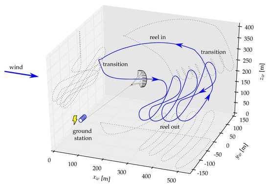
Figure 1.
Computed flight path of a kite power system using a flexible wing with suspended kite control unit and single tether (kite and drum not to scale) [13].
So far, AWE has been demonstrated only on a level of several hundred Kilowatts, i.e., one magnitude lower than what would be commercially viable for the utility sector [1,2]. However, AWE systems have several promising advantages compared to the horizontal wind turbines (HAWTs), for example, substantially lower material use for both tower structure and foundations as well as lower costs for transportation, installations and maintenance. Conventional wind turbines use the tower and foundation to transfer the bending moment of the aerodynamically loaded rotor to the ground. AWE systems use one or more tethers to transfer forces of a similar magnitude. The design, as a tensile structure, substantially reduces the material use, which leads to lower system costs and environmental footprint. It also allows for a dynamic adjustment of the operational altitude to the available wind resources, which can greatly increase the capacity factor [14]. For a HAWT, almost of the power is generated by the tip of the rotor blades while the rest of the rotor functions mainly as a support structure for the crosswind motion of the blades [1,2]. The rated power of the generator typically determines the installation. For the same rated power, an AWE system generally gives a higher annual yield than a HAWT because it can operate at a higher capacity factor. The higher capacity factor is a result of the more persistent and more steady wind at higher altitudes. However, an AWE system also needs more space than a HAWT, which increases the costs of an installation. These land surface costs are still quite unknown and responsible for the large differences in expected costs [2].
In this paper we focus on flexible membrane kites as they are less expensive, require low maintenance costs and are more safe. To maximize the power production the kite is operated in crosswind maneuvers during reel out of the tether [6]. We use a tether of constant length attached to a towing vehicle to produce a controlled relative flow environment, there is no actual drum/generator module yet. Figure 2 shows the typical system components of such an AWE system, for the example of the 20 kW technology demonstrator of Delft University of Technology. Several companies are currently developing AWE systems with flexible membrane kites: Kitenergy [15], KiteGen [16], SkySails Power [17] and Kitepower [18]. Among these the highest technology readiness level (TRL) has been reached by the company Kitepower which commercially develops a 100 KW system with a kite of 60 m wing surface area.
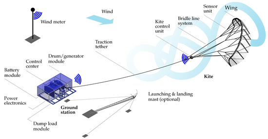
Figure 2.
Airborne wind energy system components [19].
1.2. Machine Learning Methods in AWE
Machine learning (ML) and deep learning (DL) methods have gained a lot of research momentum recently because of their capabilities in modeling nonlinear input–output relations when solving classification or regression problems. Their power extend to multivariate problems where the number of input variables, which are also known as features, is large. They have have been successfully applied in computer vision [20], pattern recognition [20], bioinformatics [21], medical diagnosis [22] etc., and are available in hardware-optimized software libraries such as Scikit Learn [23], Pytorch [24] and TensorFlow [25].
A class of ML methods that is widely used in practice is supervised learning; where pairs of the input variables and the output variable y are used to learn the input–output mapping function . The goal is to approximate the mapping function, optimizing some objective function, such that when new data are available on input (without associated output predictions), we would be able to predict the output variable for that data. A one-dimensional linear regression, for example, is the problem of fitting a line to a number of n labeled points , minimizing the some loss function, e.g., the least squares error.
There are several papers that deal with model-based AWE systems for kites [13,26,27,28] and tethered aircraft [29,30,31] as the flying devices of an AWE system, including a simulated approach for training constrained Gaussian processes models [32]; however, there is a lack of papers based on experimental measurements [33] using data-driven methods [34,35], although, system identification was used in several papers [28,36,37,38]. In a predecessor paper [39], experimental data from early flight tests was presented, but without any data analysis. In this paper, we enhanced the data collection process and performed more flight tests to collect more data, then applied machine learning algorithms to predict the power generation. To the best of our knowledge, this was the first attempt in the AWE community to employ experimental/measured data for training machine learning models, albeit the existence of many notable papers that combined the topics of machine learning and wind energy (see, e.g., [40,41,42,43]).
1.3. Contribution and Organization
In this paper we describe an AWE research platform developed at Kyushu University, covering system set-up, ground station and kite control unit (KCU). Several tests were performed to analyze the kite performance for several truck speeds and flight conditions. The tether force curves of the data obtained from the flight tests were carried and analyzed. Finally, we performed sensitivity analysis and applied several machine learning algorithms to predict the power output of the AWE system.
The paper is divided into four main sections. Section 2 presents how we collected the data, including the system set-up and the hardware used in the project. Section 3 discusses the design of the experiment and the experimental results obtained from the truck test. Then we performed data analysis, including sensitivity analysis, presented in Section 4. In Section 5 we show the construction of the machine learning and quality assessment of the model. In Section 6, we present our applied neural network and various machine learning techniques. Finally, conclusions and future work are reported in Section 7.
2. System Setup and Data Collection
The kite system of Kyushu University is a small prototype designed for 7 kW traction power. It uses an inflatable wing of 6 m surface area and a suspended remote-controlled KCU, similar to the airborne kite component depicted in Figure 2. We performed early flight tests with the KCU anchored at the ground at Nata beach, Fukuoka, Japan, as shown in Figure 3a. The wind speed during these tests was between 6 and 10 m/s. For safety reasons, we launched the kite manually from the side of the wind window, where the pulling force is relatively low. Following that, a trained human pilot operated the kite in figure-of-eight maneuvers, using the remote control (RC) of the KCU.
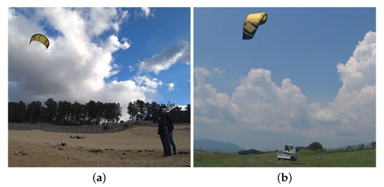
Figure 3.
Flight tests with (a) stationary kite control unit (KCU) anchored at the ground and (b) towed KCU flying on a short tether.
During these early tests we could not measure the wind speed at the kite. We also faced the problem of often having too low wind speeds to launch the kite. For these reasons, we moved to a tow test setup, tethering the KCU to a truck, as shown in Figure 3b. These tests were performed on days with only little wind to avoid a perturbation of the generated relative air flow. Under these circumstances, the apparent wind speed at the kite and the truck speed are nearly identical, which gave us another DOF to be controlled. The tests were performed on a small air field for unmanned aerial vehicles at Shiroshi, Saga, Japan, with a run way of 750 m, depicted in Figure 4.
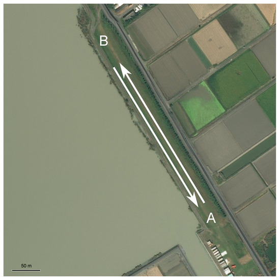
Figure 4.
Aerial view of the run way used for the tow tests, at Shiroshi, Saga, Japan (© DigitalGlobe, © Zennin).
The schematic illustration of the tow test setup in Figure 5 (Truck image: Freepik.com) details how the wing was connected to the KCU by three separate lines: the power line, which connected to the leading edge of the wing via several bridle lines, and two control lines, which connected to the wing tips at the trailing edge. The power line was kept at a constant length of 13.3 m (measured from the KCU to the end of the first fork), we used control lines of three different lengths, 13.4, 13.6 and 13.8 m, by which it was possible to adjust the angle of attack of the wing. The KCU was connected to the truck deck by a short tether with a constant length of 0.4 m. For energy harvesting in a configuration as depicted in Figure 2, the tether would be much longer to allow the kite to sweep a larger volume and to reach higher altitudes [12]. The pulling force of the wing was measured by a tension meter that is attached at the KCU.
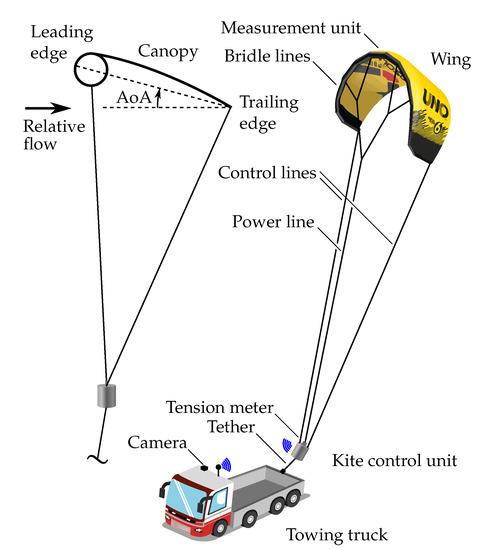
Figure 5.
Schematic illustration of the tow test setup: side view with angle of attack (AoA) definition (left) and 3D view (right).
2.1. System Components
The ground equipment included the wireless unit receiver, a speed sensor and tension meter accessories. The KCU design and its functional components are illustrated in Figure 6. The mass of the KCU, including the Lithium battery, was about 3 kg. The KCU was located 13 m below the kite and used a servo motor to actuate the control lines by which the kite was steered on a specific flight path. The employed bridle layout is common for small surf kites and supports the leading edge tube at four points, and the rear ends of the wing tips are connected to the control lines. The kite is steered by asymmetric control input, shortening one control line while feeding out the other line. Such control input leads mainly to a deformation of the wing by spanwise twisting, because the front bridle largely constrains a roll motion of the wing when the power line and the control lines are tensioned. The wing twist and the modulated aerodynamic load on the wing tips induce a yaw moment by which the kite is steered into a turn [44,45]. At the current stage of the project, it was not possible to actively control the angle of attack of the wing, however, the length of the control lines could be varied along different flight tests. The KCU receives the control action for the servo motor wirelessly from the RC. The KCU was connected to a tension meter which measures the generated pulling force during testing. The KCU was powered by a Lithium battery which could sustain almost three hours of continuous operation. The power line and the tether used in the experiment were made of Dyneema® designed for a maximum force of 2500 N.
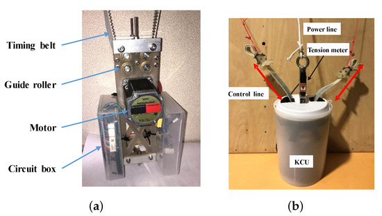
Figure 6.
Design of the KCU, including structural frame, transmission belts, electronic circuit and motors. (a) The core of the KCU without casing and (b) after putting the casing on.
As shown in Figure 7, a small measurement unit was attached to the connection of leading edge and center strut of the kite to obtain the position, height and attitude. An Arduino® microcontroller, a global positioning system (GPS), an inertial measurement unit (IMU) and pressure sensors are used to obtain this data. XBEE® was used to sent the data wirelessly to the ground station with a sampling time of 0.15 s.
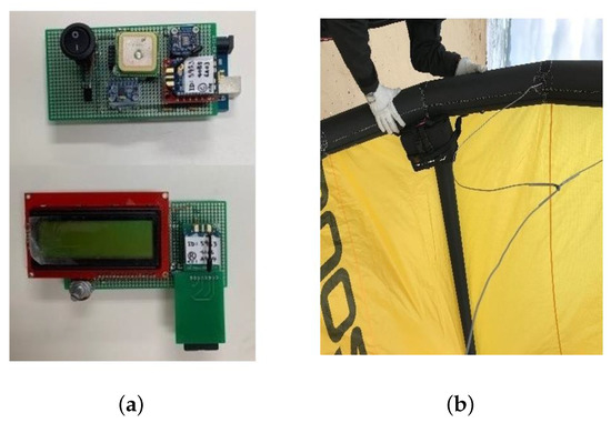
Figure 7.
(a) Measurement unit and (b) attachment on the leading edge of the kite.
2.2. Data Collection
Table 1 shows the data that were collected by the different sensors.

Table 1.
Data from sensors and statistics of the numerical attributes.
Two additional columns for the sampling time (time step) and the number of satellites (satellite count) to which the GPS is connected are included in the data, but not displayed in the table. Subsequently, we added an additional column for the maneuver type (steady flight or figure-of-eight maneuver), and an additional column for the control line length (CLL). The length difference between the control lines and the power line controls the nominal angle of attack, as shown in Figure 5 (left). The output feature is the tether force, which was measured using a tension meter. This force is one factor for power generation, the tether reeling speed, using a drum/generator module, the other factor. In the present study, this second factor was not analyzed.
In Table 1 we present some statistics for each attribute/feature of the collected data; minimum and maximum values, mean which is the central value of a discrete set of numbers: specifically, the sum of the values divided by the number of values, standard deviation (std) which measures how dispersed the values are, the 25%, median 50% and 75% rows show the corresponding percentiles: a percentile indicates the value below which a given percentage of observations in a group of observations falls.
3. Design of Experiment (DOE)
In this section we discuss the results of the tow tests. The experimental work comprises seven tests summarized in Table 2, for different combinations of towing speed, kite maneuver and control line length. The objective of these tests was to quantify the effect of these parameters on the tether force. For tests 1–4, the truck followed a continuous towing path A-B-A-B-A on the run way (see Figure 4), performing two loops. Each time the end points A or B were reached, the truck performed a U-turn at a reduced speed of 20 km/h. For tests 5–7, only a single loop was performed. During towing, the kite was either operated in figure-of-eight flight maneuvers, or kept in a steady flight state by maintaining a constant position with respect to the truck.
Table 2.
Test specifications based on truck speed, flight mode and control line length (CLL).
The results of the seven tests are presented below. Figure 8 represents a 3D visualization of the kite and truck trajectories for tests with the kite both in steady flight and performing figure-of-eight maneuvers. The effect of the crosswind maneuvering can be recognized from the evolution of the tether force for cases with similar towing speeds, as in tests 1 and 2. As shown in Figure 9, the force almost doubled and exhibited more aggressive fluctuations, when flying figure-of-eight maneuvers. On the other hand, Figure 10 shows how the tether force increases with the towing speed, considering a steady flight mode, as in tests 1 and 3. In Figure 11, Figure 12, Figure 13, Figure 14, Figure 15, Figure 16 and Figure 17, the subfigures b, c, e and f show the same sinusoidal pattern, clearly indicating the number of towing loops, which is different for tests 1–4 and tests 5–6. Figure 11, Figure 12, Figure 13, Figure 14, Figure 15, Figure 16 and Figure 17 represent the data set that we used to train and test the ML algorithm.
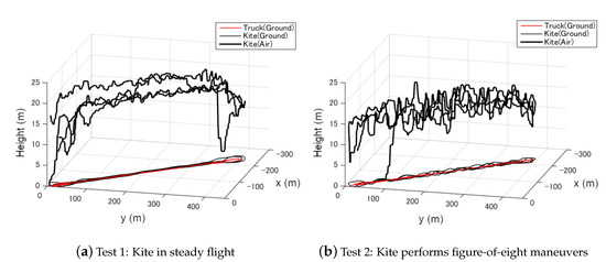
Figure 8.
A 3D visualization of the kite for tests 1 and 2.
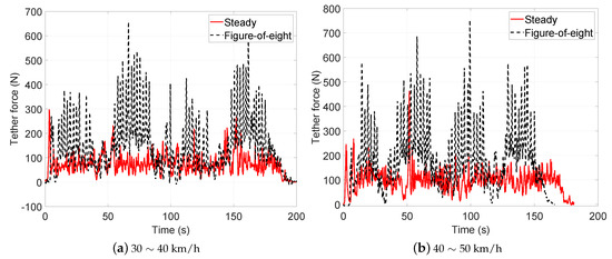
Figure 9.
Effect of flight mode for tests 1 & 2 and 3 & 4.
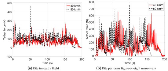
Figure 10.
Effect of towing speed for tests 1 & 3 and 2 & 4.
- Test 1: Steady flight with towing speed 30∼40 km/h and CLL = 13.8 m

Figure 11.
Data for test 1.
Figure 11.
Data for test 1.

- Test 2: Figure-of-eight maneuvers with towing speed 30∼40 km/h and CLL = 13.8 m

Figure 12.
Data for test 2.
Figure 12.
Data for test 2.

- Test 3: Steady flight with towing speed 40∼50 km/h and CLL = 13.8 m

Figure 13.
Data for test 3.
Figure 13.
Data for test 3.

- Test 4: Figure-of-eight maneuvers with towing speed 40∼50 km/h and CLL = 13.8 m

Figure 14.
Data for test 4.
Figure 14.
Data for test 4.

- Test 5: Steady flight with towing speed 30∼40 km/h and CLL = 13.6 m

Figure 15.
Data for test 5.
Figure 15.
Data for test 5.

- Test 6: Steady flight with towing speed 30∼40 km/h and CLL = 13.4 m

Figure 16.
Data for test 6.
Figure 16.
Data for test 6.

- Test 7: Steady flight with towing speed 40∼50 km/h and CLL = 13.6 m

Figure 17.
Data for test 7.
Figure 17.
Data for test 7.

4. Data Analysis and Preprocessing
In this section, we prepare and pre-process the collected measurements described in Section 3 for inclusion in the machine learning modeling work flow. Furthermore, we present a sensitivity analysis study of the relations between inputs and their impact on the output, the tether force prediction.
4.1. Handling Categorical Variables
Most of our input variables (features) are continuous or discrete, and we encode categorical ones (e.g., motion type = {Steady, FigEight}) as a one-hot numeric array. The input to this encoder could be an array of values taken on by categorical (discrete) features. The features are encoded using a one-hot (also defined as “dummy” or “one-of-K”) encoding. Consequently, each category is represented by a binary column.
4.2. Global Sensitivity Analysis
Sensitivity analysis (SA) can be defined as the study of how uncertainty in the output of a model can be apportioned to different input uncertainty sources [46]. Sensitivity analysis differs from uncertainty quantification (UQ), which characterizes output uncertainty in terms of the empirical probability density or confidence bounds. In other words, UQ aims to answer questions about how uncertain the model output is, whereas SA aims to identify the main sources of this uncertainty, per the input uncertainties. SA is typically used for model reduction, inference about various aspects of the studied phenomenon, and optimal experimental design (OED).
At a high level, sensitivity analysis can be done locally or globally. On the one hand, local SA methods examine the sensitivity of the model inputs at one specific point in the input space. Global methods, on the other hand, take the sensitivities at multiple points in the input space, before taking some measure of the average of these sensitivities.
4.3. Feature Ranking and Selection
Global sensitivity analysis is often used to select a subset of the input features. Fundamentally, these are the processes of selecting the features that can make the predicted output more accurate or eliminating those features that are irrelevant and can decrease the model accuracy and quality.
We start our analysis using an univariate feature selection approach which examines individual features, one at a time, to determine the strength of the relationship of the feature with the output prediction. A simple univariate method for understanding the relation of a feature to the output prediction variable is Pearson correlation coefficient (PCC), which measures the amount of linear correlation between two variables, resulting in a value between and 1, where means positive correlation, 0 means no linear correlation and means negative correlation (as one variable increases, the other decreases).
We computed the Pearson correlations between all variables using the Python machine learning toolbox Scikit Learn and display them as a heat map in Figure 18. The correlations with the predicted tether force (output) are illustrated in Figure 19, which is an alternative visualization of a subset of the data contained in the heat map, represented by bar chart. It indicates a stronger impact on the variability of the tether force for height, towing speed and the one-hot encoded maneuver variable (represented by the two binary variables Steady and FigEight). These remarks are consistent with our intuitive observations and experimental results, shown in Figure 9 for the maneuver type variable and Figure 10 for towing speed.
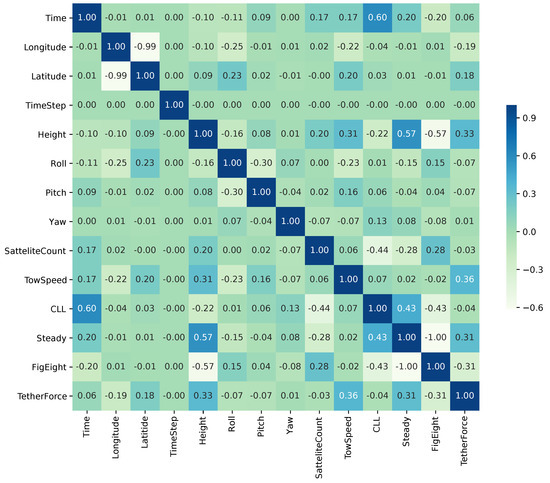
Figure 18.
Pearson correlation coefficient for tow test.
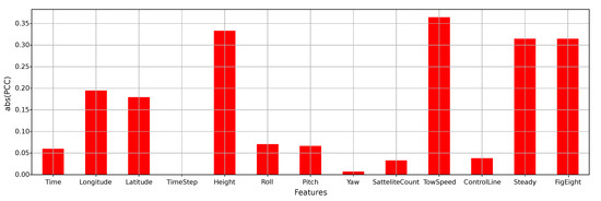
Figure 19.
Absolute value of Pearson correlation coefficient (PCC) between input features and the output prediction (tether force).
To avoid the high ranking of statistically dependent variables, we examine the correlations among the top features. The correlations between the top four features are listed in Table 3 with the output (tether force) and among each other showing relative statistical independence.
Table 3.
Pearson correlation among the top-correlated features with the tether force.
4.4. Model-Based Sensitivity Analysis
To investigate the sensitivity of the tether force for variations of the input parameters, we used the theoretical framework first derived in [6] and later expanded in [27,47]. In the first step, the tether force was formulated as
where is the air density, the resultant aerodynamic coefficient of the kite, S the wing surface area and the apparent wind velocity at the kite. Equation (1) is based on the simplifying assumption that the gravitational force acting on the kite is negligible compared to the aerodynamic force. For the following analysis we assume that the kite is towed with constant speed at constant tether length through a windless environment. We denote the wind speed relative to the towing truck as . When the kite is in a steady flight mode, the apparent wind velocity is identical to the generated wind speed
and from Equation (1) we find
When flying crosswind maneuvers, the apparent wind velocity at the kite is given by
where is the elevation angle, the azimuth angle and the lift-to-drag ratio of the kite. Equation (4) follows from ([47], Equation (2.15)) for the special case of a constant tether length and negligible gravitational force contributions. The theoretical framework can be expanded to include the effect of gravity ([47], Equation (2.67)), which is beyond the scope of this analysis. The term quantifies the angular deviation of the tether from the wind speed vector that is created by the towing of the kite, and the square root is an amplification term resulting from the crosswind maneuvering of the kite. The higher the lift-to-drag ratio of the kite, the higher its flight speed and apparent wind speed. By inserting Equation (4) into Equation (1) we get, for the tether force
The model parameters determining the tether force are related to sensor data as follows. For the kite in steady flight mode, Equation (3) suggests that the only sensor data with influence on the tether force is the wind speed (TowSpeed) that is generated by the towing of the kite. On the other hand, this speed is kinematically coupled to the sensor data Longitude, Latitude and Time. Because of the diagonal orientation of the run way (see Figure 4) we can expect a roughly equal correlation of the tether force to Longitude and Latitude. For the kite flying crosswind maneuvers, Equation (5) suggests an additional influence of the maneuvering, expressed by the factor . The bracketed amplification factor depends on the aerodynamic performance of the kite, which was not considered as a variable in this study.
To illustrate this for the example of a kite with a lift-to-drag ratio , which is typical for this size of kite with additional line drag included. When this kite is flying crosswind maneuvers at an elevation angle of the tether force experiences an amplification by a factor of 10, which is contributed by the aerodynamic term, while the maneuvering term reduces this amplification again by a factor of . The joint effect is a maximum force increase by a factor of , compared to the case of steady towing. Roughly such an increase can be observed in the measured tether forces shown in Figure 9.
5. Regression Model Construction
In this section, we constructed initial regression models of different types, approximating the output tether force. We then used quality metrics to assess the predictions.
5.1. Multivariate Regression
Regression as a predictive modeling technique investigates the relationship between the inputs and the output of a model. The accuracy of a regression model depends on the model order and the types of input and output data. For example, linear regression fits a linear model to the known data points in order to minimize the residual sum of squares between the labeled training outputs and the predictions made by the linear approximation. Common regressors include neural networks, linear regressors, support vector machines and decision trees.
We considered neural network models along with other regression methods such as linear regression, decision trees and gradient boosting. These models differ in accuracy and we, therefore, used standard statistical metrics to compare their performance under the same training data set.
5.2. Quality Metrics
To assess the performance of the machine learning algorithm, we split our data set into two subsets, training and test sets, which contain 70% and 30% of the samples, respectively, as shown in Figure 20.
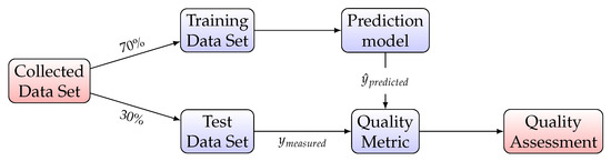
Figure 20.
Assessing the performance of machine learning to build a predictive model.
After training the model, we developed a formula to predict the tether force. Because we use 12 different features, this formula is very complex and for this reason we will not display it in this paper. We used this formula to predict the tether force for the test set and then compared this prediction to the measured tether force that is already part of the test set. This quantitative comparison was based on quality metrics, which have the role of a cost functions. An algorithm such as the gradient descent algorithm was used to minimize the quality metrics. There are several quality metrics that can be used as a test score for model validation. Our choices are stated in the following, denoting as the predicted value of the i-th sample, as the corresponding true value, n as the number of samples and as variance.
- Mean Square Error: expected value of the squared (quadratic) error
- Coefficient of Determination (): represents the proportion of variance (of y) that has been explained by the independent variables in the model, providing an indication of goodness of fit and therefore a measure of how well unseen samples are likely to be predicted by the model, through the proportion of explained variancewhere and . Best possible score is 1 and it can be negative, because the model can be arbitrarily worse. A constant model that always predicts the expected value of y, disregarding the input features, would get a score of 0.
- Maximum Residual Error: captures the worst case error between the predicted value and the true value. In a perfectly fitted single output regression model, it would be 0 on the training set. This metric shows the extent of error that the model had when it was fitted
- Explained Variance: best possible score is 1, lower values are worse.
- Mean Absolute Error: expected value of the absolute error loss or -norm loss
6. ML Experimental Results
In our experiments, we used the aggregated data from all seven tests in Table 2. We start by running basic neural networks experiments and follow with comparisons to other multivariate regression models.
6.1. Neural Network Regression
Neural network models have gained a lot of research attention due to their capabilities in modeling nonlinear input–output relations. In general, neural networks work similarly to the human brain’s neural networks. A “neuron” in a neural network is a mathematical function that collects and classifies information according to some pre-determined architecture, achieving statistical objectives such as curve fitting and regression analysis.
In terms of architecture, a neural network contains layers of interconnected nodes. Figure 21 illustrates the tether force prediction problem as a neural network with two hidden layers. Each node is a perceptron and is similar to a multiple linear regression. The perceptron feeds the signal produced by a multiple linear regression into an activation function that may be nonlinear. In a multi-layered perceptron (MLP), perceptrons are arranged in interconnected layers. The input layer collects input patterns. The output layer has classifications or output signals to which input patterns may map. In our work, our predicted output is the tether force. Hidden layers fine-tune the input weightings until the neural network’s margin of error is minimal. It is hypothesized that hidden layers extrapolate salient features in the input data that have predictive power regarding the outputs.
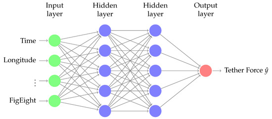
Figure 21.
A neural network illustration of tether force prediction with two hidden layers.
We used the TensorFlow and Keras [48] libraries to create a regression-based neural network with linear activation functions. At a high level, an activation function determines the output of a learning model, its accuracy and also the computational efficiency of the training a model. It can generally be designed to be linear or nonlinear to reflect the complexity of the predicted function.
For exploration, we used two hidden layers of 12 and 8 neurons, respectively, over 500 optimization iterations (epochs, forward and backward passes). A model summary is reported in Table 4 highlighting the dimensions of dense layers, the number of parameters to be optimized in each epoch per layer and the total number of trainable parameters.
Table 4.
Keras model summary.
For a small network of two layers with 12/8 neurons, a total number of 281 parameters need to be trained. This number grows quickly as the number of layers and neurons per layer increases. Although adding layers/neurons would clearly improve the prediction accuracy, it obviously comes with an added computational cost. Trade-off studies are often used to find a practical implementation with acceptable accuracy, for a given training data set.
Figure 22 highlights the decreasing training and validation losses along epochs. Once the model was trained to a satisfactory error metric, we used it for predicting tether force values of new input vectors.
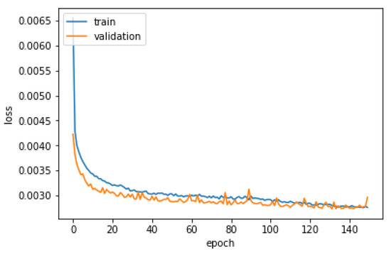
Figure 22.
Neural network model loss performance, based on mean squared error (MSE).
6.2. Comparing Regression Models
To further demonstrate the value of machine learning regression models for an accurate prediction of the power output of airborne wind energy systems, we evaluated different standard regression models per the quality metrics in Section 5.2, along with the training time. We used standard Scikit Learn implementations. Results are reported in Table 5. For this study, we split the full data set into random train and test subsets, we used for training and save for testing.
Table 5.
Quality metrics of different regression models.
A key remark at this point is that no one model scores best for all data sets in terms of all quality metrics. Multiple iterations and hyper-parameter tuning operations would be needed for further model optimization. We note the different trade-offs highlighted in Table 5, e.g., between training time and accuracy [49].
For example, linear regression is one of the simplest algorithms trained using gradient descent (GD), which is an iterative optimization approach that gradually tweaks the model parameters to minimize the cost function over the training set. A linear model might not have the best accuracy but is simple to implement and hence is best of quick domain exploration. It makes a prediction by computing a weighted sum of the input features, plus a constant called the bias term , where is the hypothesis function and is the model’s parameter vector containing the bias term and the feature weights to .
Regularization is often used to further improve the loss function optimization. On the one hand, ridge regression is a regularized version of linear regression where a regularization term equal to is added to the cost function. This forces the learning algorithm to not only fit the data but also keep the model weights as small as possible. The hyper-parameter controls how much you want to regularize the model. If , then ridge regression is just a linear regression. If is very large, then all weights end up very close to zero and the result is a flat line going through the data’s mean. On the other hand, lasso regression is another regularized version of linear regression that adds a regularization term to the cost function, but uses the norm of the weight vector instead of half the square of the norm; like this . Lasso regression tends to completely eliminate the weights of the least important features (i.e., set them to zero), in other words, it automatically performs feature selection and outputs a sparse model (i.e., with few nonzero feature weights). Elastic net regression is a middle ground between ridge regression and lasso regression. The regularization term is a simple mix of both ridge and lasso regularization terms, and you can control the mix ratio r. When , elastic net is equivalent to ridge regression, and when , it is equivalent to lasso regression.
Despite their longer training times, nonlinear models are expected to perform better for our data set. As we noticed in Figure 11, Figure 12, Figure 13, Figure 14, Figure 15, Figure 16 and Figure 17, input features and output force are not linearly related. To start, polynomial regression introduces nonlinearity by imposing powers of each feature as new features. It then trains a linear model on this extended set of features.
Alternatively, ensemble learning methods use a group of predictors, voting amongst them for the best performance; and hence are often called voting regression. The accuracy of voting regression depends on how powerful each predictor is in the group and their independence. Finally, boosting refers to any ensemble method that combines several weak learners into a strong learner. The general idea of most boosting methods is to train predictors sequentially, each trying to correct its predecessor, often resulting in the best performance, compared to individual models. Due to the limitation of training data, voting among multiple regressors yielded higher accuracy (less MSE) compared to individual models, as shown in Table 5. If more training data is available, optimizing a single model to outperform ensemble models would be feasible.
Per our machine learning experiments, we could conclude the clear success of a neural network model applied to AWE for predicting tether force, even without hyper-parameter tuning. The main model drawback is that it takes a longer training time than other algorithms, despite its overall accuracy performance.
A major advantage for our ML model is cost. Once a model is trained, there is no need to physically run new experiments (with the same test setup, as shown in Figure 5), to predict the tether force. Instead, we could simply rely on our current NN model to predict the estimated tether force for new input combinations. We could use our gradient boosting model, if we care about evaluation/prediction time, rather than model accuracy. Note that the evaluation time is the time required to calculate the predicted tether force from our model (prediction formula). The neural network generates a more accurate formula, but also more complex and takes more time for evaluation.
7. Conclusions and Future Work
In this work, we demonstrated a novel approach to employ machine learning regression methods, based on experimental measurements, for the prediction of the power generated by AWE systems. Using an experimental kite system designed at Kyushu University, we orchestrated seven design scenarios of different input specifications. We used experimentally-collected numerical and categorical data from multiple sensors to construct multivariate regression models to predict the generated tether force.
- Our sensitivity analysis results have validated our intuitive understanding of measurement ranking in impacting the predicted tether force, and hence the generated power.
- The performance of different ML algorithms was assessed, including neural networks, linear regression and ensemble methods, in terms of training time and different accuracy metrics. Different regression algorithms resulted in different performance scores, emphasizing the need for further studies around the training data set and hyperparameter tuning.
- Our preliminary investigations highlighted the potential of ML modeling methods in predicting tether force and traction power in AWE applications.
In future work, we will leverage the significance of height and type of motion (steady flight and figure-of-eight flight maneuvers) to the accuracy of the multivariate regression models into exploring new trajectories for improved/optimal power generation. We will also attempt to overcome different types of measurement errors by improving the data collection procedures by including:
- the steering actuation of the KCU, either directly measured as a linear motion of the control lines, or derived from the rotation of the motor,
- the apparent wind speed at the kite,
- the angle of attack of the apparent wind velocity vector with the wing, and
- the side slip angle of the apparent wind velocity vector with the wing.
We will also use information that we gain from our ML model to actively determine optimal deployment locations for AWE systems.
Author Contributions
Software, M.A.R. and A.A.R.; data collection, T.N.D., M.A.R. and A.M.H.; design of experiment, M.A.R., A.A.R., T.N.D. and S.Y.; writing—original draft preparation, M.A.R. and A.A.R.; writing—review and editing, M.A.R. and R.S.; supervision and funding acquisition, S.Y. and R.S. All authors have read and agree to the published version of the manuscript.
Funding
M.A.R. conducted this work with the support of Japanese Ministry of Education, Culture, Sports, Science and Technology (MEXT). R.S. was supported by the H2020-ITN project AWESCO funded by the European Union’s Horizon 2020 research and innovation programme under the Marie Skłodowska-Curie grant agreement No. 642682. The Open Access publication of this manuscript was funded by TU Delft.
Acknowledgments
Sandia National Laboratories is a multimission laboratory managed and operated by National Technology & Engineering Solutions of Sandia, LLC, a wholly owned subsidiary of Honeywell International Inc., for the U.S. Department of Energy’s National Nuclear Security Administration under contract DE-NA0003525. This paper describes objective technical results and analysis. Any subjective views or opinions that might be expressed in the paper do not necessarily represent the views of the U.S. Department of Energy or the United States Government.
Conflicts of Interest
The authors declare no conflict of interest.
Data Availability
The data set used for this study is available for download from https://doi.org/10.4121/uuid:c3cee766-2804-4c00-924f-8a9f6c8122fc.
References
- Schmehl, R. (Ed.) Airborne Wind Energy: Advances in Technology Development and Research; Green Energy and Technology; Springer: Singapore, 2018. [Google Scholar]
- Ahrens, U.; Diehl, M.; Schmehl, R. (Eds.) Airborne Wind Energy; Green Energy and Technology; Springer: Berlin/Heidelberg, Germany, 2013. [Google Scholar]
- Cherubini, A.; Papini, A.; Vertechy, R.; Fontana, M. Airborne Wind Energy Systems: A review of the technologies. Renew. Sustain. Energy Rev. 2015, 51, 1461–1476. [Google Scholar] [CrossRef]
- Mendonça, A.K.D.S.; Vaz, C.R.; Lezana, Á.G.R.; Anacleto, C.A.; Paladini, E.P. Comparing patent and scientific literature in airborne wind energy. Sustainability 2017, 9, 915. [Google Scholar] [CrossRef]
- Samson, J.; Katebi, R.; Vermillion, C. A critical assessment of airborne wind energy systems. In Proceedings of the 2nd IET Renewable Power Generation Conference, Beijing, China, 9–11 September 2013; pp. 4–7. [Google Scholar]
- Loyd, M.L. Crosswind kite power (for large-scale wind power production). J. Energy 1980, 4, 106–111. [Google Scholar] [CrossRef]
- Ockels, W.J. Laddermill, a novel concept to exploit the energy in the airspace. Aircr. Des. 2001, 4, 81–97. [Google Scholar] [CrossRef]
- Williams, P.; Lansdorp, B.; Ockesl, W. Optimal crosswind towing and power generation with tethered kites. J. Guid. Control Dyn. 2008, 31, 81–93. [Google Scholar] [CrossRef]
- Cherubini, A.; Vertechy, R.; Fontana, M. Simplified model of offshore airborne wind energy converters. Renew. Energy 2016, 88, 465–473. [Google Scholar] [CrossRef]
- AWESCO Network. Airborne Wind Energy—An Introduction to an Emerging Technology. Available online: http://www.awesco.eu/awe-explained (accessed on 14 February 2020).
- Fagiano, L.; Zgraggen, A.U.; Morari, M.; Khammash, M. Automatic crosswind flight of tethered wings for airborne wind energy: Modeling, control design, and experimental results. IEEE Trans. Control Syst. Technol. 2013, 22, 1433–1447. [Google Scholar]
- Van der Vlugt, R.; Peschel, J.; Schmehl, R. Design and Experimental Characterization of a Pumping Kite Power System. In Airborne Wind Energy; Ahrens, U., Diehl, M., Schmehl, R., Eds.; Green Energy and Technology; Springer: Berlin/Heidelberg, Germany, 2013; Chapter 23; pp. 403–425. [Google Scholar]
- Fechner, U. A Methodology for the Design of Kite-Power Control Systems. Ph.D. Thesis, Delft University of Technology, Delft, The Netherlands, 2016. [Google Scholar]
- Bechtle, P.; Schelbergen, M.; Schmehl, R.; Zillmann, U.; Watson, S. Airborne Wind Energy Resource Analysis. Renew. Energy 2019, 141, 1103–1116. [Google Scholar] [CrossRef]
- Kitenergy S.r.l. Available online: http://www.kitenergy.net/ (accessed on 14 February 2020).
- KiteGen S.r.l. Available online: http://www.kitegen.com/en/ (accessed on 14 February 2020).
- Skysails Power GmbH. Available online: https://skysails-power.com/ (accessed on 14 February 2020).
- Kitepower B.V. Available online: https://kitepower.nl/ (accessed on 14 February 2020).
- Salma, V.; Friedl, F.; Schmehl, R. Reliability and Safety of Airborne Wind Energy Systems. Wind Energy 2019, 23, 340–356. [Google Scholar] [CrossRef]
- Bishop, C.M. Pattern Recognition and Machine Learning; Springer: New York, NY, USA, 2006. [Google Scholar]
- Baldi, P.; Brunak, S. Bioinformatics: The Machine Learning Approach, 2nd ed.; MIT Press: Cambridge, MA, USA, 2001. [Google Scholar]
- Kourou, K.; Exarchos, T.P.; Exarchos, K.P.; Karamouzis, M.V.; Fotiadis, D.I. Machine learning applications in cancer prognosis and prediction. Comput. Struct. Biotechnol. J. 2015, 13, 8–17. [Google Scholar] [CrossRef]
- Pedregosa, F.; Varoquaux, G.; Gramfort, A.; Michel, V.; Thirion, B.; Grisel, O.; Blondel, M.; Prettenhofer, P.; Weiss, R.; Dubourg, V.; et al. Scikit-learn: Machine learning in Python. J. Mach. Learn. Res. 2011, 12, 2825–2830. [Google Scholar]
- Paszke, A.; Gross, S.; Chintala, S.; Chanan, G.; Yang, E.; DeVito, Z.; Lin, Z.; Desmaison, A.; Antiga, L.; Lerer, A. Automatic differentiation in PyTorch. In Proceedings of the 31st Conference on Neural Information Processing Systems (NIPS 2017), Long Beach, CA, USA, 4–9 December 2017. [Google Scholar]
- Abadi, M.; Barham, P.; Chen, J.; Chen, Z.; Davis, A.; Dean, J.; Devin, M.; Ghemawat, S.; Irving, G.; Isard, M.; et al. Tensorflow: A system for large-scale machine learning. In Proceedings of the 12th {USENIX} Symposium on Operating Systems Design and Implementation ({OSDI} 16), Savannah, GA, USA, 2–4 November 2016; pp. 265–283. [Google Scholar]
- Rushdi, M.; Yoshida, S.; Dief, T.N. Simulation of a Tether of a Kite Power System Using a Lumped Mass Model. In Proceedings of the International Exchange and Innovation Conference on Engineering & Science (IECES), Fukuoka, Japan, 18–19 October 2018; pp. 42–47. [Google Scholar]
- Van der Vlugt, R.; Bley, A.; Schmehl, R.; Noom, M. Quasi-Steady Model of a Pumping Kite Power System. Renew. Energy 2019, 131, 83–99. [Google Scholar] [CrossRef]
- Dief, T.N.; Fechner, U.; Schmehl, R.; Yoshida, S.; Rushdi, M.A. Adaptive Flight Path Control of Airborne Wind Energy Systems. Energies 2020, 13, 667. [Google Scholar] [CrossRef]
- Rapp, S.; Schmehl, R.; Oland, E.; Haas, T. Cascaded Pumping Cycle Control for Rigid Wing Airborne Wind Energy Systems. J. Guid. Control Dyn. 2019, 42, 2456–2473. [Google Scholar] [CrossRef]
- Rushdi, M.; Hussein, A.; Dief, T.N.; Yoshida, S.; Schmehl, R. Simulation of the Transition Phase for an Optimally-Controlled Tethered VTOL Rigid Aircraft for Airborne Wind Energy Generation. In Proceedings of the AIAA Scitech 2020 Forum, Orlando, FL, USA, 6–10 January 2020. [Google Scholar]
- Licitra, G. Identification and Optimization of an Airborne Wind Energy System. Ph.D. Thesis, University of Freiburg, Breisgau, Germany, 2018. [Google Scholar]
- Diwale, S.S.; Lymperopoulos, I.; Jones, C.N. Optimization of an airborne wind energy system using constrained gaussian processes. In Proceedings of the 2014 IEEE Conference on Control Applications (CCA), Nice, France, 8–10 October 2014; pp. 1394–1399. [Google Scholar]
- Oehler, J.; Schmehl, R. Aerodynamic characterization of a soft kite by in situ flow measurement. Wind Energy Sci. 2019, 4, 1. [Google Scholar] [CrossRef]
- Baheri, A.; Vermillion, C. Altitude optimization of airborne wind energy systems: A Bayesian optimization approach. In Proceedings of the 2017 American Control Conference (ACC), Seattle, WA, USA, 24–26 May 2017; pp. 1365–1370. [Google Scholar]
- Wood, T.A.; Hesse, H.; Smith, R.S. Predictive control of autonomous kites in tow test experiments. IEEE Control Syst. Lett. 2017, 1, 110–115. [Google Scholar] [CrossRef]
- Licitra, G.; Bürger, A.; Williams, P.; Ruiterkamp, R.; Diehl, M. System Identification of a Rigid Wing Airborne Wind Energy System. arXiv 2017, arXiv:1711.10010. [Google Scholar]
- Licitra, G.; Koenemann, J.; Bürger, A.; Williams, P.; Ruiterkamp, R.; Diehl, M. Performance assessment of a rigid wing Airborne Wind Energy pumping system. Energy 2019, 173, 569–585. [Google Scholar] [CrossRef]
- Dief, T.N.; Fechner, U.; Schmehl, R.; Yoshida, S.; Ismaiel, A.M.; Halawa, A.M. System identification, fuzzy control and simulation of a kite power system with fixed tether length. Wind Energy Sci. 2018, 3, 275–291. [Google Scholar] [CrossRef]
- Dief, T.N.; Rushdi, M.; Halawa, A.; Yoshida, S. Hardware-in-the-Loop (HIL) and Experimental Findings for the 7 kW Pumping Kite Power System. In Proceedings of the AIAA Scitech 2020 Forum, Orlando, FL, USA, 6–10 January 2020. [Google Scholar]
- Clifton, A.; Kilcher, L.; Lundquist, J.; Fleming, P. Using machine learning to predict wind turbine power output. Environ. Res. Lett. 2013, 8, 024009. [Google Scholar] [CrossRef]
- Heinermann, J.; Kramer, O. Machine learning ensembles for wind power prediction. Renew. Energy 2016, 89, 671–679. [Google Scholar] [CrossRef]
- Treiber, N.A.; Heinermann, J.; Kramer, O. Wind power prediction with machine learning. In Computational Sustainability; Lässig, J., Kersting, K., Morik, K., Eds.; Springer: Cham, Switzerland, 2016; Volume 645, pp. 13–29. [Google Scholar]
- Ti, Z.; Deng, X.W.; Yang, H. Wake modeling of wind turbines using machine learning. Appl. Energy 2020, 257, 114025. [Google Scholar] [CrossRef]
- Breukels, J. An Engineering Methodology for Kite Design. Ph.D. Thesis, Delft University of Technology, Delft, The Netherlands, 2011. [Google Scholar]
- Bosch, A.; Schmehl, R.; Tiso, P.; Rixen, D. Dynamic nonlinear aeroelastic model of a kite for power generation. J. Guid. Control Dyn. 2014, 37, 1426–1436. [Google Scholar] [CrossRef]
- Saltelli, A.; Ratto, M.; Andres, T.; Campolongo, F.; Cariboni, J.; Gatelli, D.; Saisana, M.; Tarantola, S. Global Sensitivity Analysis: The Primer; John Wiley & Sons: Hoboken, NJ, USA, 2008. [Google Scholar]
- Schmehl, R.; Noom, M.; van der Vlugt, R. Traction Power Generation with Tethered Wings. In Airborne Wind Energy; Green Energy and Technology; Ahrens, U., Diehl, M., Schmehl, R., Eds.; Springer: Berlin/Heidelberg, Germany, 2013; Chapter 2; pp. 23–45. [Google Scholar]
- Chollet, F. Keras: The Python Deep Learning Library. Available online: https://keras.io (accessed on 23 March 2020).
- Géron, A. Hands-On Machine Learning with Scikit-Learn, Keras, and TensorFlow: Concepts, Tools, and Techniques to Build Intelligent Systems, 2nd ed.; O’Reilly Media: Sebastopol, CA, USA, 2019. [Google Scholar]


© 2020 by the authors. Licensee MDPI, Basel, Switzerland. This article is an open access article distributed under the terms and conditions of the Creative Commons Attribution (CC BY) license (http://creativecommons.org/licenses/by/4.0/).