Pan-European CVaR-Constrained Stochastic Unit Commitment in Day-Ahead and Intraday Electricity Markets

Abstract

The fundamental modeling of energy systems through individual unit commitment decisions is crucial for energy system planning. However, current large-scale models are not capable of including uncertainties or even risk-averse behavior arising from forecasting errors of variable renewable energies. However, risks associated with uncertain forecasting errors have become increasingly relevant within the process of decarbonization. The intraday market serves to compensate for these forecasting errors. Thus, the uncertainty of forecasting errors results in uncertain intraday prices and quantities. Therefore, this paper proposes a two-stage risk-constrained stochastic optimization approach to fundamentally model unit commitment decisions facing an uncertain intraday market. By the nesting of Lagrangian relaxation and an extended Benders decomposition, this model can be applied to large-scale, e.g., pan-European, power systems. The approach is applied to scenarios for 2023—considering a full nuclear phase-out in Germany—and 2035—considering a full coal phase-out in Germany. First, the influence of the risk factors is evaluated. Furthermore, an evaluation of the market prices shows an increase in price levels as well as an increasing day-ahead-intraday spread in 2023 and in 2035. Finally, it is shown that intraday cross-border trading has a significant influence on trading volumes and prices and ensures a more efficient allocation of resources.

1. Introduction

The global societal goal of limiting global warming leads to policies for increasing the share of renewable energies (REN) in the gross final energy consumption to 27% in the EU and 30% in the Federal Republic of Germany by 2030 [1,2,3,4]. The expansion of REN, dominated by wind energy (WTG) and photovoltaics (PV), takes place mainly in the electricity sector [5,6]. Their supply-dependent generation leads to ex-ante uncertain generation volumes. The expected feed-in is marketed on the day-ahead market (DA), which allows for trading on an hourly basis. The DA market is organized as an auction which takes place on 12 p.m. on the day before delivery. To compensate for forecasting errors from trading on the DA market, the intraday market (ID) was introduced in 2007. 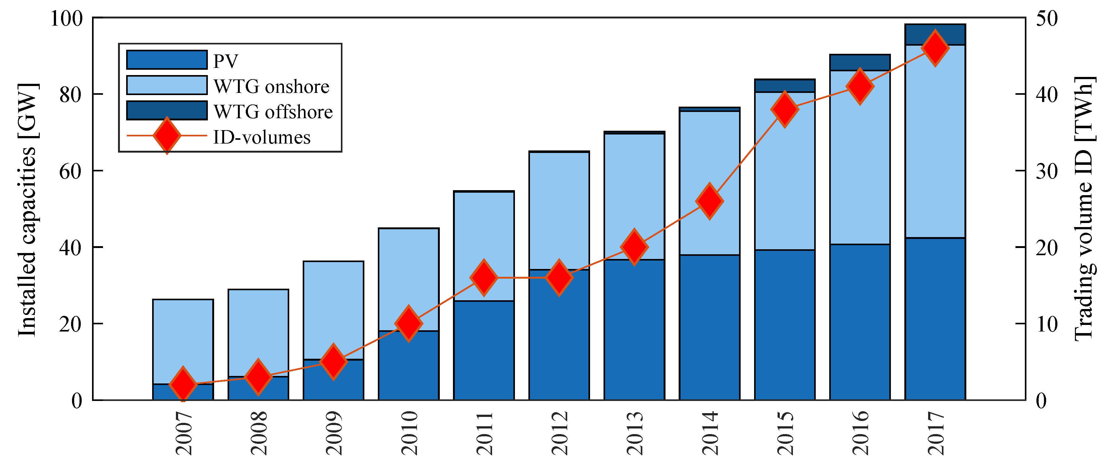It allows for the possibility of re-trading up to five minutes before delivery [7]. In contrast to the DA market, trading on the ID market, except for the ID opening auction, takes place as continuous trading. Moreover, it is possible to trade on a quarter hourly basis on the ID market. In proportion to the increase in variable renewable energies (VRE) in recent years, the absolute forecasting errors and thus the trading volume and liquidity on the ID market have grown steadily by 40% per year on average (see Figure 1) [8]. Over the same period, the volume traded on the DA market has grown by an average of 12% per year [8]. However, while the ID market has steadily grown in trading volume from year to year, there has been a decline in trading volumes on the DA market in 2013, 2016 and 2017 [8]. In total, the trading volume on the DA market increased by two and a half times in 10 years and by twenty-two times on the ID market [8]. While the ID market accounted for only 2% of the trading volume of the DA market in 2007, this share has now grown to 21%.

Even if the forecasting quality improves, this development will be further reinforced by the expected REN expansion rates [9]. Participation in the ID market is becoming increasingly important due to high price volatility and the resulting opportunities, especially for flexible power plants as they are often no longer viable on the DA market [10]. In addition to attractive revenue opportunities, power plants face a significant risk exposure on the volatile ID market. For example, in 2016 the volatility (defined as the hourly price difference relative to the base price) of the DA market price returns is 11.5% whereas the volatility of the ID market is 12.3%. (We applied that measure according to [11] for the volatility because electricity prices close or equal to zero result in extremely large price returns, if calculated according to the common practice. Thus, the usual standard deviation as a measure of the volatility of such returns would not be reliable.).

Modeling the power system’s behavior bottom-up is vital to evaluating regulatory interventions, strategic decisions for market participants and energy system planning. Due to the crucial importance in the decision-making process of power plants and the functionality of the market design, the consideration of the ID market is highly relevant for bottom-up modeled electricity market models. This results in the following core characteristics that such an approach has to take into consideration: Power plant operators face a two-stage decision-making process when operating in the spot market. The optimal bid for the DA market has to take into account all possible ID price scenarios and their associated risks. Due to the ex-ante uncertain ID volumes and prices, this results in a stochastic two-stage decision-making process. In addition, the integration of risk metrics becomes necessary, since economic decision makers generally act in a risk-averse manner [12,13,14]. Furthermore, the consideration of both the detailed techno-economic power plant parameters, e.g., start-up costs, and the market-coupling of power markets within the European interconnected power system (ENTSO-E area) is essential for the model quality [15].

Several bottom-up approaches model the unit commitment (UC) in large-scale energy systems. Additionally, some models further calculate the associated electricity market prices. Beside bottom-up approaches, statistical approaches for modeling ID prices were proposed [16], which are inherently not applicable for long-term forecasting. As outlined in [17], available bottom-up approaches can be divided into deterministic models (omitting the stochasticity of the VRE), and stochastic models:

• Deterministic mathematical optimization approaches: A wide range of electricity market models use mathematical optimization to generate individual power plant schedules simulating the interconnected pan-European power system or rather its electricity markets [18,19,20,21]. Some not only use simplified linear models but also include detailed constraints resulting in mixed integer problems allowing for UC decisions [15,22,23,24]. Simplified multistage decisions are rarely taken into account as they are insignificant if uncertainty is neglected [25]. Those decisions usually comprise a coarse yearly energy planing, which is subsequently updated by a finer monthly energy planing and finally adjusted by an hourly unit commitment.
• Stochastic meta-heuristic approaches: Meta-heuristic approaches are often used if mathematical optimization becomes computationally critical but lacks the guarantee of optimality. Paradoxically, the only applications of such models in the literature so far are small test systems [26,27,28].
• Stochastic mathematical optimization approaches: In contrast to meta-heuristic approaches, mathematical optimization guarantees an optimal solution, if the problem is convex, and in contrast to meta-heuristics, also transparent and parametrization-independent. The included uncertainties can be modeled as i.i.d. [29,30,31,32], or modeled time-dependently, either through Markov-chains [33] or time series analysis approaches [34,35,36,37,38]. The computational burden of high-dimensional models can be reduced by applying scenario reduction methods, which are partly integrated in existing approaches [39,40,41,42]. The integration of risk measures associated with the depicted uncertainties results in a significant increase in computational complexity; therefore such approaches are still used in test systems only [30,31,42]. There are hardly any approaches considering complex power plant restrictions depending on integer decision variables, such as start-up costs, minimum down/up times, or minimum load so far. These constraints were approximated through linear formulations in [39]. In addition to the unit schedules, a price signal is also necessary in electricity market models to enable subsequent economic assessments. However, it is of crucial importance that modeled prices and modeled unit schedules are mutually coherent, i.e., that the resulting market signal can reflect the behavior of market participants without distortion. This requires detailed modeling of the causal relationships, so that, for example, the influence of start-up costs on electricity prices can be represented [34,40]. The number of variables and constraints in a mathematical optimization model of a stochastic unit commitment formulation grow linearly with the number of considered scenarios, thus requiring extensive computing resources. Therefore, market zones considered in the literature are predominantly limited to test networks or small supply areas [29,30,31,32,33,34,38,40,42]. So far, only publications based either on the Wilmar Joint Market Model [35,36,39] or a second approach [41] allow the representation of real-scale systems such as the German or Irish market areas [37], albeit without integer related and thus complex restrictions.

In summary, established real-scale electricity market models do not encompass uncertainties because of the computational complexity. Stochastic approaches based on mathematical optimization can only be applied to real-scale systems if relevant power plant parameters are simplified. As a result, there is currently no procedure for simulating the electricity market, taking into account short-term forecast uncertainties, and depicting real decision-making processes of market participants. The modeling of this two-stage decision situation requires the integration of a risk measure, so that the indifference between uncertain and secure returns can be resolved. The consideration of detailed power plant characteristics using unit commitment approaches is important for reproducing realistic operation behavior. Likewise, the endogenous consideration of the interconnections of all markets in the European integrated grid is indispensable to reproduce the market design.

This paper presents an approach to model large-scale, detailed electricity spot markets, taking into account the uncertainties of renewable energy forecasts and the electrical system load. For this purpose, the unit commitment decisions are modeled bottom-up, i.e., for each hydro-thermal power plant greater than ten megawatts. This allows the consideration of power plant-specific characteristics that reflect the technical and economic constraints. In addition, the modeling of the real decision calculus under uncertainty—i.e., The optimal distribution of marketing volumes between the DA and ID market—is made possible by integrating risk aversion into the decision process individually for each plant. The impact of international electricity trading on national market results is significant, which is why all market areas within the European interconnected grid are considered. In contrast to the current state of research, the following process for bottom-up modeling DA and ID markets is derived: The forecast uncertainties of VRE and the system load are modeled using methods of time series analysis and scenario reduction. The two-stage decision-making process for large power plants is realistically represented in a mathematical optimization process, taking into account the conditional value-at-risk (CVaR) as a risk measure. The inclusion of complex technical and economic constraints in power plant operation is necessary [43], as such restrictions play a major role in real-life-commitment decisions. The implicit market coupling of trading capacities across all market areas within the European interconnected grid must be taken into account in the decision-making process [44].

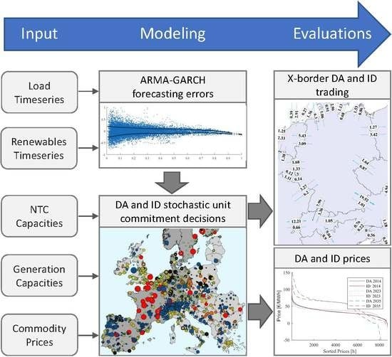
The remainder of the paper is organized as follows. Section 2 gives a brief overview of modeling the forecasting errors for wind, pv and load, which represent the ID volumes in the bottom-up electricity market simulation. In Section 3, an existing Lagrangian relaxation approach is extended to a stochastic two-stage approach, where the modeled units optimize against a certain DA price and an uncertain ID price. The (European) ID market is based on continues trading, whereas an overall system-optimizing model corresponds to the characteristics of an auction. Nonetheless, it is permissible to model the ID market without distorting the results because, especially for larger markets such as the spot market, both market forms (auction-based and continuous trading) converge into one another [45,46,47]. We therefore conclude that the continuous ID market can be approximated by optimization models. Due to the functional relationship between the forecast error and the price spread between the DA and ID markets, which can be observed in empirical studies, it can be deduced that the ID market can be modeled by defining forecasting errors as the dominating trading volume [48].

The stochastic Lagrangian approach is further extended in Section 4 through the integration of the CVaR as a risk measure that enables modeling risk-averse behavior of power plants. The block-angular structure of the thermal power plants allows for applying Benders decomposition, although the coupling CVaR-constraint is further complicating. Therefore, an extended Benders decomposition approach is developed in Section 5 and applied to a scenario envisioning the power system in 2023 and in 2035 in Section 6. The paper concludes with a summary and an outlook in Section 7.

2. Modeling Forecasting Errors

ID trading was created to integrate VRE, i.e., to compensate for forecasting errors [49,50]. Assuming a steadily increasing cumulative supply function, it follows that forecasting errors traded on the ID market lead to a price difference between the DA and ID markets. This relationship can be shown empirically [48]. Thus, the bottom-up modeling of the ID market requires the modeling of forecasting errors. In addition to the VRE forecasting errors, which mainly consist of errors in the wind and PV forecasts, the electrical load also has a stochastic character. On this basis, the present approach generates the ID volume from the modeled forecasting errors of PV, wind and electric load.

We use empirical data on day-ahead feed-in forecasts and actual feed-in from 2015–2016 on the basis of transparency data supplied by EEX to determine the empirical forecasting error [51]. For this purpose, we do not use the absolute forecasting errors, but the forecasting errors related to the forecast. The forecasting error distributions are standardized by removing the offset (expected value) and normalized to the standard deviation of one. This enables us to later roll out the findings gained later on forecast time series for future scenarios. The time series of the forecasting errors are first examined for deterministic components. We have shown that the time series of the forecasting errors have a purely stochastic character and can be modeled using time series analysis methods [52]. Furthermore, a dependence of the distribution moments of the forecasting error on the forecast, a dependence of the forecasting error on itself, and a time-dependent variance of the forecasting error was determined. The dependencies properties can be categorized as follows:

• Dependent moments: The expected value and especially the standard deviation or dispersion of the normalized forecast errors depend on the forecast level of the underlying time series.
• Autoregression: The level of the current forecasting error depends on the past forecasting errors—it is auto-correlated. The reason for this lies in the fact that on the DA market all 96 quarter hours of the following day are traded simultaneously and are therefore based on the same forecast. However, a cross-correlation, such as for example a dependency of the forecasting error of wind, on the forecasting error of PV, cannot be determined.
• Heteroskedasticity: Even after filtering the standard deviation caused by the forecast level, a non-variance-stationary process remains, i.e., a time series with time-dependent standard deviation.

The following is a brief overview of the modeling of forecasting errors focusing on optimal ARMA-GARCH model orders (by using [53]) and optimal scenario quantities. For a better understanding of the context and a more detailed description of the model formulations and the results, we refer to [52].

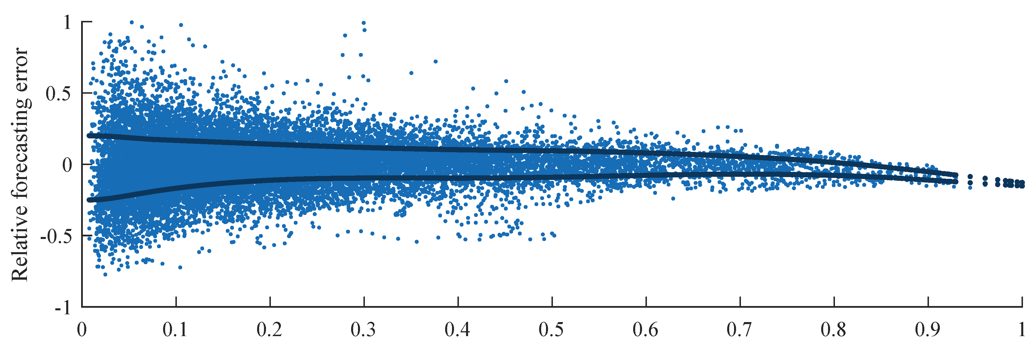
Despite the absence of classical trends and seasonal effects, we have identified a dependence of the forecast error on the feed-in forecast (see Figure 2). Both the mean error and the variance of the error depend on the forecast level. Using regression analysis we were able to filter this dependence from the data. For estimation, we use multivariate adaptive regressions splines (MARS) (by using [54]), because they can estimate the nonlinear dependence on linear polygon trajectories [55,56]. (The regressand is the amplitude of the predicted feed or load. An optimal number of basis functions, each for wind, PV and load, was found to be 12 [52]. A further increase of the basic functions leads to the non-monotonous behavior of the resulting polygons, which seems counter-intuitive. The parameter estimation provides the coefficients of the basis functions and the parameters of the associated hockey stick functions of the MARS model, which are used for the later deconvolution of the simulated forecasting errors [52]).

The residual of the MARS filtering shows an autocorrelation which is subsequently filtered by fitting ARMA-models to the residual. A method for evaluating the significance of parameters in regression models are statistical tests, especially the evaluation of the p-value. However, it is advised that model selection itself and therefore the amount and combination of the relevant parameters should be based on other measures, such as cross evaluation or information criteria or cross-validation [57]. 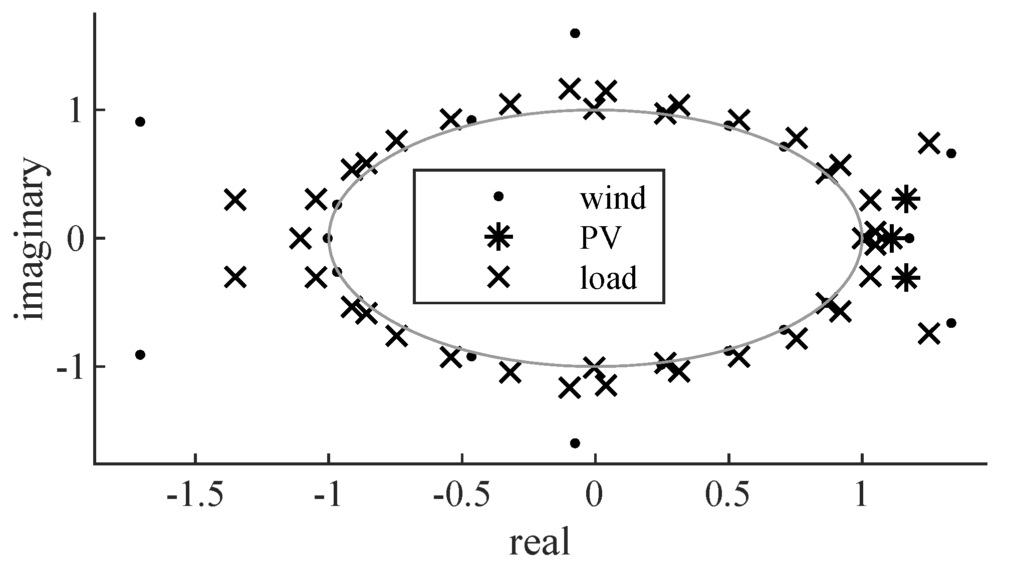Therefore, the model selection (different parameter settings) in this paper was performed using the SBIC information criterion [58]. This leads to an ARMA(21,15) model for wind, an ARMA(3,3) model for PV and an ARMA(40,10) model for the load capturing the autocorrelation (The parameters of the ARMA models are shown in

Table A1. Parameter for ARMA models for wind, pv, and load.

Lag	Wind		PV		Load
	AR	MA	AR	MA	AR	MA
1	4.192	−2.876	0.743	−0.002	1.962	−0.961
2	−9.618	5.366	0.772	−0.790	−2.494	1.443
3	15.303	−6.839	−0.542	−0.018	2.725	−1.193
4	−18.879	7.214			−1.626	0.304
5	19.610	−6.648			1.203	−0.794
6	−18.852	6.419			−1.395	0.602
7	18.475	−6.634			1.521	−0.874
8	−19.025	7.081			−2.109	1.217
9	19.878	−7.281			1.693	−0.430
10	−20.120	7.042			−0.930	0.410
11	19.440	−6.531			0.419
12	−17.541	5.358			−0.024
13	14.241	−3.821			0.007
14	−9.726	1.929			−0.042
15	5.137	−0.678			0.063
16	−1.799				−0.039
17	0.227				0.009
18	0.120				0.045
19	−0.115				−0.022
20	0.065				0.020
21	−0.017				−0.034
22					0.064
23					−0.104
24					0.200
25					−0.257
26					0.243
27					−0.251
28					0.112
29					−0.066
30					0.104
31					−0.095
32					0.182
33					−0.111
34					−0.019
35					0.097
36					−0.152
37					0.119
38					−0.068
39					0.032
40					−0.013

and the stability test of the AR term in Figure A1 in the Appendix A). The absence of autocorrelation in the ARMA filtering residuals, which is a necessary condition for a sufficiently estimated model, is proven by applying the Ljung Box portmanteau test.

However, the ARMA residuals show heteroskedastic behavior, proven by an ARCH-test, so that after the ARMA filtering a GARCH filtering is performed (The parameters of the GARCH models are shown in

Table A2. Parameter of GARCH(1,1) models for wind, pv and load, where $\omega$ is the constant, $\alpha$ the arch coefficient and $\beta$ the garch coefficient.

Wind			PV			Load
$\mathit{\omega }$	$\mathit{\alpha }$	$\mathit{\beta }$	$\mathit{\omega }$	$\mathit{\alpha }$	$\mathit{\beta }$	$\mathit{\omega }$	$\mathit{\alpha }$	$\mathit{\beta }$
0.043	0.197	0.568	0.017	0.135	0.778	0.348	0.645	0.077

in the Appendix A). A GARCH(1,1)-model was shown in the literature to be the superior model order (cf. [59]) and is therefore singled out for this paper. An ARCH test carried out again after the GARCH filtering shows that the GARCH residuals show homoscedastic behavior and therefore the filtering is sufficient.

Finally, the GARCH residuals follow a white noise process and are approximated using a theoretical Student’s t-distribution, so that they can be sampled afterward.

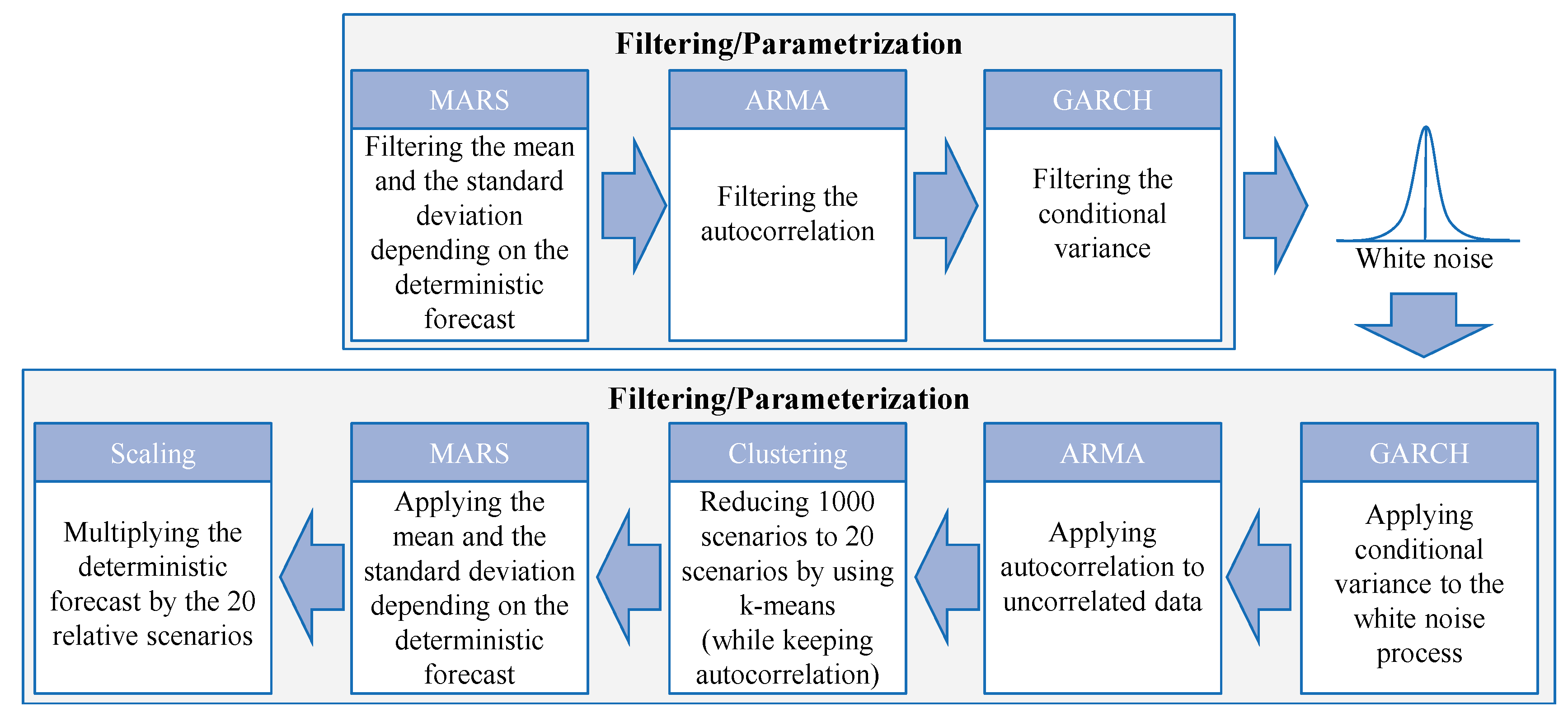
To simulate forecasting errors, the process is performed in reverse. For this purpose, a scenario is generated by sampling from the theoretical distribution. The time series generated in this way corresponds to white noise, shows no autocorrelation and is homoscedastic. The heteroscedastic property is then implanted by applying the previously estimated GARCH process. In the same way, the autocorrelative property is implanted subsequently by applying the previously estimated ARMA process. This Monte Carlo simulation generates an hourly time series for an entire simulation year is performed n times to generate n scenarios. In the following, the ID market is modeled on an hourly basis, analogous to the DA market, and is therefore aggregated here from the quarter-hourly products to hourly products. The modeling quality can be determined by measuring the distance between the simulated distribution (from the Monte-Carlo simulation) and the empirical distribution (relative forecasting errors in 2015 and 2016). This finding is needed to determine the necessary number of scenarios, or what added value the addition of more scenarios provides. A metric that measures the equality of two distribution functions is the Hellinger distance [60]. 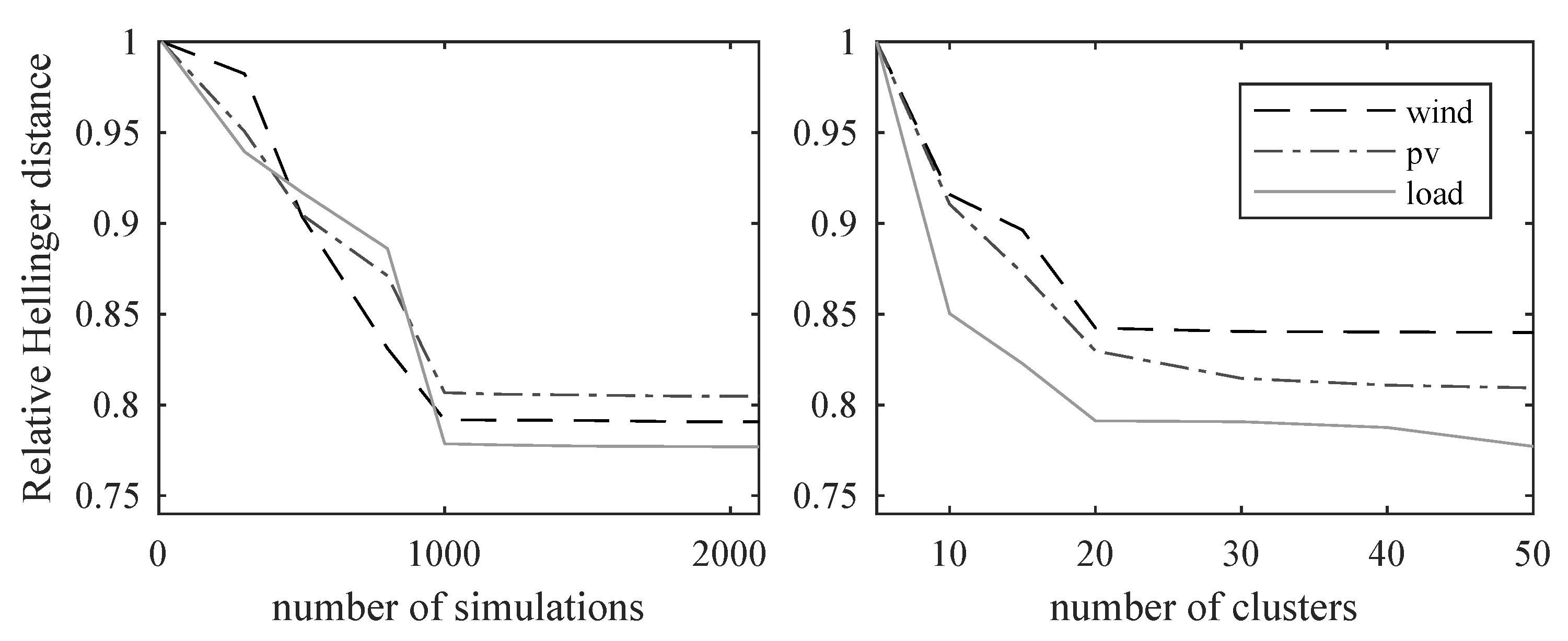It proposed to be a valid metric for comparing probability distributions especially in weather models [61]. By comparing the marginal benefit of adding further scenarios increases steeply at first, but only marginally from 1000 scenarios onwards (see Figure 3). This information can be used as a measure which indicates that 1000 Monte Carlo simulations for wind, PV and load being the best trade-off between the accuracy and model parsimony. This principle is comparable to the so-called elbow criterion from cluster analysis [60]. Another possibility for model selection are scoring rules, which, related to the divergence function proposed here, evaluate the model quality over the distance between a modeled random variable and empiric realizations [62,63].

To reduce the n scenarios, the k-Means algorithm is chosen from the class of partitioning cluster procedures. It selects k-clusters in such a way that the Euclidean distance between the scenarios and the resulting cluster centroids is minimal. Usually, the resulting cluster centroids are chosen as the archetype for the cluster and are reused. However, the cluster centers of gravity distort the properties modeled above, such as conditional moments, autocorrelation, and heteroskedasticity, to such an extent that they become obsolete. Therefore, the scenario with the smallest Euclidean distance to the cluster center of gravity is chosen as the archetype of the cluster. The relative Hellinger distance and the elbow criterion suggest 20 clusters as the best balance between considered scenarios and parsimony (see Figure 3). This procedure, therefore, results in 20 clusters or scenarios, which are time series selected from the pool of Monte Carlo simulated time series. They thus include both the autocorrelations modeled using ARMA and the conditional variance modeled using GARCH. Their probability is derived from the ratio of the time series assigned to a cluster from the k-means clustering. The generated scenarios are then transferred to a future year by multiplying the deterministic forecast time series for wind, PV and load by the 20 associated stochastic scenarios. The workflow of the process is shown in Figure 4.

3. Lagrangian Relaxation of the Pan-European Unit Commitment Problem

Bottom-up energy system models based on UC approaches are usually designed as optimization problems to minimize the total system’s costs [15]. In reality, however, electricity generation is not provided via a centrally planned-economy approach, but is freely traded on the market. Nonetheless, market participants in markets with full competition and uniform pricing offer at marginal cost, so that, with approximate full competition, the real market and a cost-minimizing overall planning approach converge into the same market outcome [64]. 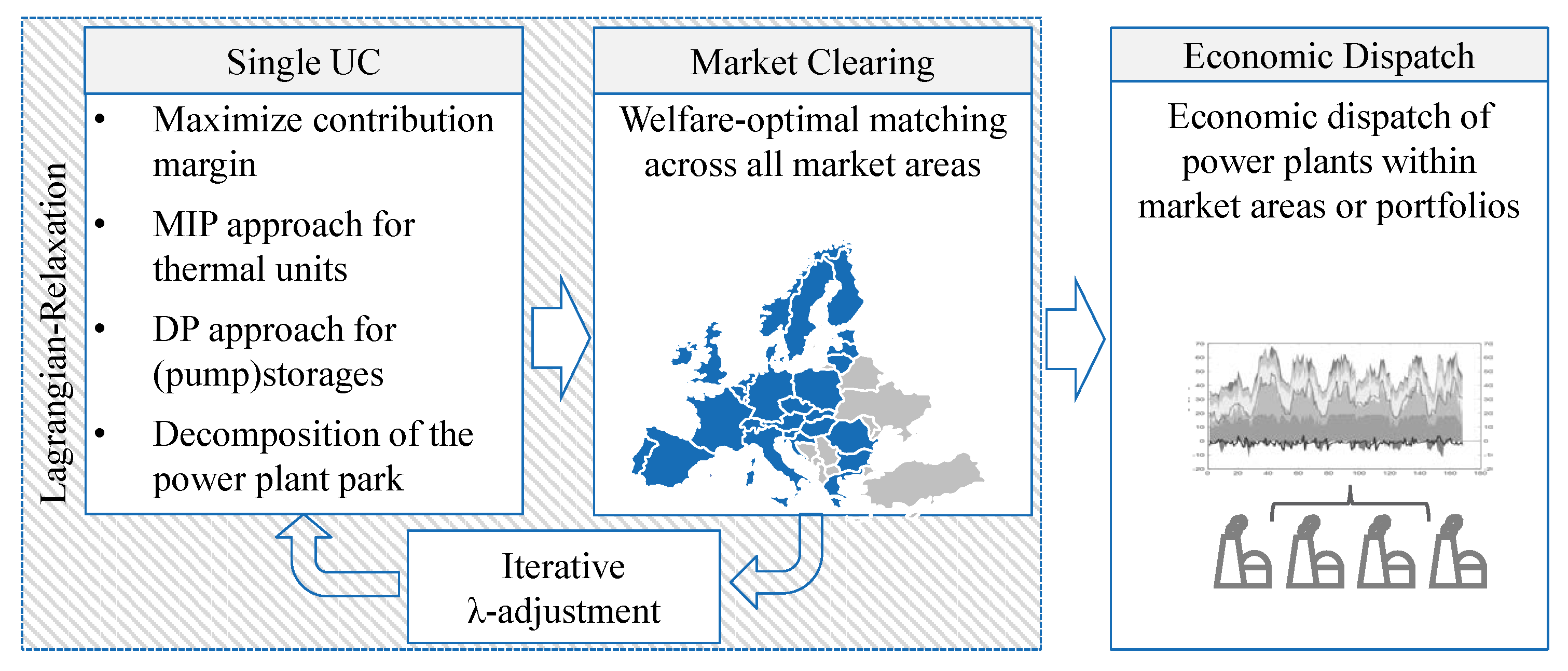The approach developed in [15] is an UC approach, which solves the cost minimal load coverage across all ENTSO-E market areas by applying Lagrangian relaxation while simultaneously considering market coupling. This enables decoupled optimization of individual power plants against a shadow price. The commitment of thermal units is determined by a mixed-integer linear programming (MILP) approach and the hydraulic units by a dynamic programming (DP) approach, whereas distributed generation is determined exogenously. The bids of the units are auctioned at welfare-optimal pricing by means of a market coupling algorithm based on the EUPHEMIA algorithm [65], which is used in the European spot market. In the update of the Lagrangian multipliers, unused transmission capacities resulting from market coupling are taken into account so that cross-border trading is integrated within the Lagrangian process (flowchart see Figure 5).

The integration of the ID market into a unit commitment optimization model by considering forecasting errors can be realized through a two-stage linear stochastic programming approach [14] (for readability, decision variables are denoted bold within the following optimization problem formulations). The first-stage consists of the deterministic part of objective function $g^T\mathit{x}$ subject to the set of constraints from (3). The second-stage, the stochastic part, consists of the ${\pi }_{\omega }$-weighted objective functions $q_{\omega }^T{\mathit{y}}_{\omega }$ representing a set $\Omega$ of discrete scenarios. The second stage is subject to the recourse matrix W and the technology matrix ${\mathcal{T}}_{\omega }$, which in sum must correspond to the vector $h_{\omega }$. The latter, ${\mathcal{T}}_{\omega }$, couples first stage decisions to the second stage.

$$\begin{array}{c}\underset{\mathit{x},{\mathit{y}}_{\omega }}{min}{g}^{\mathrm{T}}\mathit{x}+\sum _{\omega \in \Omega }{\pi }_{\omega }{q}_{\omega }^{\mathrm{T}}{\mathit{y}}_{\omega }\hfill \end{array}$$

(1)

$$\begin{array}{c}\mathrm{s}.\mathrm{t}.\hfill \end{array}$$

(2)

$$\begin{array}{cc}\hfill A\mathit{x}& \le b\hfill \end{array}$$

(3)

$$\begin{array}{cc}\hfill {\mathcal{T}}_{\omega }\mathit{x}+W{\mathit{y}}_{\omega }& =h_{\omega },\omega \in \Omega \hfill \end{array}$$

(4)

$$\begin{array}{cc}\hfill \sum _{\omega \in \Omega }{\pi }_{\omega }& =1\hfill \end{array}$$

(5)

$$\begin{array}{c}\hfill \mathit{x}\ge 0,{\mathit{y}}_{\omega }\ge 0,\omega \in \Omega \end{array}$$

(6)

Applying this generic structure to the pan-European unit commitment problem, where the DA-load is considered ex-ante certain and the ID-load ex-ante uncertain, leads to the following objective function, with K single units in C markets with a simulation horizon of T time steps:

$$min\sum _{c\in C}\sum _{k\in K_c}\sum _{t\in T}\underset{\text{DA-Costs}\left({\mathit{x}}_{k,t}^{\mathrm{DA}}\right)}{\underbrace{\phantom{{\sum }_{\omega \in \Omega }}\left(a_k{\mathit{\nu }}_{k,t}^{\mathrm{DA}}+{\mathit{suc}}_{k,t}^{\mathrm{DA}}\right)}}+\sum _{c\in C}\sum _{k\in K_c}\sum _{t\in T}\underset{\text{Expected ID-Costs}\left({\mathit{y}}_{k,t,\omega }^{\mathrm{ID}}\right)}{\underbrace{{\sum }_{\omega \in \Omega }{\pi }_{\omega }\left(m_{k,t}{\mathit{P}}_{k,t,\omega }^{\mathrm{Phy}}\right)}}.$$

(7)

The binary commitment decision ${\mathit{\nu }}_{k,t}^{\mathrm{DA}}$ (with $\mathit{\nu }\in \mathbb{B}=\{0,1\}$) is calculated in the first stage causing fixed costs $a_k$ and, if the unit is switched on (${\mathit{\nu }}_t=0\to {\mathit{\nu }}_{t+1}=1$), causing start costs ${\mathit{suc}}_{k,t}^{\mathrm{DA}}$. The start-up costs are usually set depending on the current down time of the power plant. For the sake of brevity, the extensive formulation of this and other techno-economic unit constraints is omitted in this paper but can be found in [43]. The unit’s physical power output ${\mathit{P}}_{k,t,\omega }^{\mathrm{Phy}}$ is calculated within the second-stage for each probability-weighted scenario considering linear marginal costs of generation $m_{k,t}$. Moreover, the (positive or negative) bids on the DA ${\mathit{P}}_{k,t}^{\mathrm{DA}}$ and ID market ${\mathit{P}}_{k,t,\omega }^{\mathrm{ID}}$ market must correspond to the sum of its physical output (The market bids are not relevant for the here displayed objective function as their coefficients equal zero). Therefore, power plant operators are subject to a make-or-buy decision on how to fulfil their DA schedule in each scenario $\omega$:

$$\begin{array}{cc}\hfill {\mathit{P}}_{k,t}^{\mathrm{DA}}+{\mathit{P}}_{k,t,\omega }^{\mathrm{ID}}={\mathit{P}}_{k,t,\omega }^{\mathrm{Phy}},& \hfill c\in C,k\in K_c,t\in T,\omega \in \Omega .\end{array}$$

(8)

The central constraints of the optimization problem are the load balancing constraints (9) and (10), ensuring that the power output of all endogenously optimized units equals the system load $D_{c,t}^{\mathrm{DA}/\mathrm{ID}}$ including exogenously defined REN-feed-in ${\mathit{EE}}_{c,t}^{\mathrm{DA}/\mathrm{ID}}$ and market coupling decisions ${\mathit{MC}}_{c,t}^{\mathrm{DA}/\mathrm{ID}}$.

$$\begin{array}{ccc}\hfill D_{c,t}^{\mathrm{DA}}& =\sum _{k\in K_c}{\mathit{P}}_{k,t}^{\mathrm{DA}}+{\mathit{EE}}_{c,t}^{\mathrm{DA}}+{\mathit{MC}}_{c,t}^{\mathrm{DA}},\hfill & c\in C,t\in T\hfill \end{array}$$

(9)

$$\begin{array}{ccc}\hfill D_{c,t,\omega }^{\mathrm{ID}}& =\sum _{k\in K_c}{\mathit{P}}_{k,t,\omega }^{\mathrm{ID}}+{\mathit{EE}}_{c,t,\omega }^{\mathrm{ID}}+{\mathit{MC}}_{c,t,\omega }^{\mathrm{ID}},\hfill & c\in C,t\in T,\omega \in \Omega .\hfill \end{array}$$

(10)

Furthermore, each additionally considered scenario leads to a quadratic increase of the MILP’s size, which represents a key influencing factor for its solvability and computing time. Therefore, Langrangian relaxation according to [15] is applied to parallelize power plant optimization and advanced by integrating its stochastic extension to

$$\begin{array}{c}{\displaystyle \underset{{\mathit{\lambda }}_{c,t}^{\mathrm{DA}},{\mathit{\lambda }}_{c,t,\omega }^{\mathrm{ID}}}{max}}\{min{\displaystyle \sum _{c\in C}\sum _{k\in K_c}\sum _{t\in T}}\left(a_k{\mathit{\nu }}_{k,t}^{\mathrm{DA}}+{\mathit{suc}}_{k,t}^{\mathrm{DA}}\right)+{\displaystyle \sum _{c\in C}\sum _{k\in K_c}\sum _{t\in T}\sum _{\omega \in \Omega }}{\pi }_{\omega }{m}_{k,t}{\mathit{P}}_{k,t,\omega }^{\mathrm{Phy}}\\ -{\displaystyle \sum _{c\in C}\sum _{t\in T}}{\mathit{\lambda }}_{c,t}^{\mathrm{DA}}\left({\displaystyle \sum _{k\in K_c}}{\mathit{P}}_{k,t}^{\mathrm{DA}}+{\mathit{EE}}_{c,t}^{\mathrm{DA}}+{\mathit{MC}}_{c,t}^{\mathrm{DA}}-D_{c,t}^{\mathrm{DA}}\right)\\ -{\displaystyle \sum _{c\in C}\sum _{t\in T}\sum _{\omega \in \Omega }}{\pi }_{\omega }{\mathit{\lambda }}_{c,t,\omega }^{\mathrm{ID}}\left({\displaystyle \sum _{k\in K_c}}{\mathit{P}}_{k,t,\omega }^{\mathrm{ID}}+{\mathit{EE}}_{c,t,\omega }^{\mathrm{ID}}+{\mathit{MC}}_{c,t,\omega }^{\mathrm{ID}}-D_{c,t,\omega }^{\mathrm{ID}}\right)\}.\end{array}$$

(11)

$${\mathit{\lambda }}_{c,t}^{\mathrm{DA}},{\mathit{\lambda }}_{c,t,\omega }^{\mathrm{ID}}\in \mathbb{R}\text{:}\text{Lagrangian-Multiplier}\mathrm{DA}/\mathrm{ID}$$

The contribution margin of each single unit is maximized (corresponds to minimizing the unit’s costs) subject to its specific Lagrangian multipliers. The Lagrangian multipliers $\mathit{\lambda }$ of a relaxed demand constraint can be interpreted as uniform market prices [66]. Subsequently, the Langrangian multipliers are adjusted in an iterative process using a subgradient approach until convergence is achieved. Convergence is defined here when the deviation between the load on the DA market and within the ID-scenarios compared to the aggregated power plant bids on those markets drops below a threshold value. To account for realistic bidding behavior of power plants in ID markets, the risk aversion in the uncertain markets need to be taken into account. Therefore, the risk-averse stochastic UC formulation is outlined in the following section.

4. Risk-Averse Stochastic Unit Commitment

Each power plant subproblem $k\in K_c$ can be optimized independently in each Lagrangian iteration with regard to the Lagrangian multipliers $\lambda$:

$$min\sum _{t\in T}\left(a_k{\mathit{\nu }}_{k,t}^{\mathrm{DA}}+{\mathit{suc}}_{k,t}^{\mathrm{DA}}-{\lambda }_{c,t}^{\mathrm{DA}}{\mathit{P}}_{k,t}^{\mathrm{DA}}\right)+\sum _{t\in T}\sum _{\omega \in \Omega }{\pi }_{\omega }\left(m_{k,t}{\mathit{P}}_{k,t,\omega }^{\mathrm{Phy}}-{\lambda }_{c,t,\omega }^{\mathrm{ID}}{\mathit{P}}_{k,t,\omega }^{\mathrm{ID}}\right).$$

(12)

In the following, indices for market areas c and units k are omitted for brevity since only a single power plant model is considered. The objective function according to (12) leads to an optimization of the expected value and assuming risk-neutral behavior of the power plant operator.

However, power plant operators act risk-averse and thus try to limit potential losses on the ID-market by integrating suitable risk measures into their marketing decision process. This paper models this decision process through an optimization approach. The CVaR is a coherent risk measure and therefore suitable for limiting risks in optimization problems [67]. It can be interpreted as the conditional mean of the cost distribution Z greater than the $\alpha$-quantile. This $\alpha$-quantile is named value at risk (VaR). The CVaR of a random variable R is then given by

$$CVa{R}^{\alpha }\left(R\right)=inf\left\{Va{R}^{\alpha }\left(R\right)+\frac{1}{1-\alpha }\mathbb{E}\left({[R-Va{R}^{\alpha }\left(R\right)]}_{+}\right)\right\},$$

(13)

where ${[R-Va{R}^{\alpha }\left(R\right)]}_{+}=max(R-Va{R}^{\alpha }\left(R\right),0)$ and the infimum is reached at a $\alpha$-quantile of R according to [68].

Let $z(\mathit{x},\omega )$ be the objective value resulting in a specific scenario $\omega$

$$z(\mathit{x},\omega )=\underset{\text{DA-Part}}{\underbrace{{\displaystyle \sum _{t\in T}}\left(a·{\mathit{\nu }}_t^{\mathrm{DA}}+{\mathit{suc}}_t^{\mathrm{DA}}-{\lambda }_t^{\mathrm{DA}}{\mathit{P}}_t^{\mathrm{DA}}\right)}}+\underset{\text{ID-Part}Q(\mathit{x},\omega )}{\underbrace{{\displaystyle \sum _{t\in T}}\left(m_t·{\mathit{P}}_{t,\omega }^{\mathrm{Phy}}-{\lambda }_{t,\omega }^{\mathrm{ID}}{\mathit{P}}_{t,\omega }^{\mathrm{ID}}\right)}},$$

(14)

then the risk neutral behavior follows through the inherent optimization of the expected value as in (12)

$$Z_{\mathbb{E}}\left(\mathit{x}\right)=\mathbb{E}\left(z\left(\mathit{x}\right)\right).$$

(15)

Risk averse behavior can be achieved by additively integrating the CVaR into the objective function weighted by the coefficient $\beta$:

$$Z_{CVaR}\left(\mathit{x}\right)=\mathbb{E}\left(z\left(\mathit{x}\right)\right)+\beta ·{\mathrm{CVaR}}^{\alpha }\left(z\left(\mathit{x}\right)\right).$$

(16)

The translation invariance of the CVaR allows for the integration of (16) into (12) as follows:

$$\begin{array}{cc}\hfill Z_{CVaR}\left(\mathit{x}\right)=& (1+\beta )\sum _{t\in T}\left(a·{\mathit{\nu }}_t^{\mathrm{DA}}+{\mathit{suc}}_t^{\mathrm{DA}}-{\lambda }_t^{\mathrm{DA}}{\mathit{P}}_t^{\mathrm{DA}}\right)\hfill \\ & +\sum _{\omega \in \Omega }\sum _{t\in T}{\pi }_{\omega }\left(m_t·{\mathit{P}}_{t,\omega }^{\mathrm{Phy}}-{\lambda }_{t,\omega }^{\mathrm{ID}}{\mathit{P}}_{t,\omega }^{\mathrm{ID}}\right)+\beta ·{\mathrm{CVaR}}^{\alpha }\left(Q\left(\mathit{x}\right)\right).\hfill \end{array}$$

(17)

with ${\mathrm{CVaR}}^{\alpha }\left(Q\left(\mathit{x}\right)\right)$ according to [68,69]:

$${\mathrm{CVaR}}^{\alpha }\left(Q\left(\mathit{x}\right)\right)={\mathit{VaR}}^{\alpha }+\frac{1}{1-\alpha }\sum _{\omega \in \Omega }{\pi }_{\omega }{\mathit{\eta }}_{\omega }$$

(18)

$${\mathit{\eta }}_{\omega }\ge \sum _{t\in T}\left(m_t·{\mathit{P}}_{t,\omega }^{\mathrm{Phy}}-{\mathit{\lambda }}_{t,\omega }^{\mathrm{ID}}{\mathit{P}}_{t,\omega }^{\mathrm{ID}}\right)-{\mathit{VaR}}^{\alpha },\omega \in \Omega$$

(19)

$${\mathit{VaR}}^{\alpha }\in \mathbb{R},{\mathit{\eta }}_{\omega }\ge 0.$$

(20)

In this formulation, ${\mathit{VaR}}^{\alpha }$ is a decision variable that models the $Va{R}^{\alpha }\left(Q\left(\mathit{x}\right)\right)$ endogenously. The VaR over the different scenarios depends on the ex-ante unknown first-stage decision x and thus needs to be modeled endogenously. It was shown in [68,69] that this variable formulation corresponds to the analytical VaR.

To optimize large time horizons, i.e., yearly optimizations in hourly resolution, a rolling optimization scheme is applied where the optimization time horizon for each power plant k is divided into time slices. Each time time slice $\kappa$ is then solved after one another with an overlap to account for future earning opportunities in the following time slice $\kappa +1$. The length of the time slices is determined based on the physical ramping constraints of power plants as well as minimum downtimes. We have thus used a slice length of one week with an overlap of three days which was empirically shown to be appropriate. Therefore, 52 time slices are calculated for each power plant. Furthermore, the variables describing the physical state of the power plant (physical output, on/off decisions) at the beginning of the overlap are transferred to the next time slice to model the time-dependency of each scenario. Each physical intraday decision is thus conditional on the previous time slice decision in that scenario. For example, a power plant that is at its maximum power output in one scenario $\omega$ at the beginning of an overlap t is still considered to be at maximum power in that scenario $\omega$ at the beginning t of the next time slice $\kappa +1$.

The resulting optimization problem of thermal power plants for each time slice is intractable as a closed problem due to the binary start-up decisions. Therefore, in the subsequent Section 5, a decomposition method for the complex subproblems of thermal units is developed.

In contrast to thermal power plants, hydraulic power plants exhibit different characteristics, which have a significant impact on the modeling. Hydraulic power plants do not require integer decision variables, and the modeling of seasonal effects is essential. Therefore, the storages for DA operation are solved in a non-decomposed way for a whole year using DP. For the integration of the ID market, it is not possible to transform the overall problem into a two-level stochastic (linear) problem, because a decomposition in the time domain would leave seasonal effects unconsidered and a non-decomposed LP is not manageable due to the complex time-coupling constraints. Therefore a two-stage approach is applied.

First, an annual energy planning of the storage unit over the entire simulation period is carried out using DP. The results of the energy planning are the specific turbine and pumping schedules of the storage power plants in the individual hours and the resulting filling level curves of the storage basins. In the second stage, the levels are fixed at the start and endpoints of sub-intervals of the simulation period and transferred as boundary values to a linear optimization model, taking ID decisions into account. The hydraulic power plants can thus adapt their schedules to the marketing opportunities on both markets within the fixed storage limits. Thus, the filling levels of the storage reservoirs at the support points remain the same but can be varied in between. It was shown that for these problems that a Benders-decomposition does not offer any advantages concerning the solution time, which can be explained by the fact that pure LPs can be solved very efficiently by solvers despite the addition of the ID market as a closed linear program according to the structure in Figure 6.

5. Benders Decomposition of Thermal Power Plants

The above introduced power plant model shows a block-angular structure of the constraint matrix, which comprises both decision stages according to (3) and (4) (see Figure 6). Therefore, one part of the constraints—represented by the matrix A and the right-hand side b—exclusively refer to the first-stage, i.e., DA, variables, whereas other constraints—represented by the matrices $T_{\omega }$ and W and the right-hand side $h_{\omega }$—have to be satisfied conjointly and are thus coupling the ID decisions per scenario $\omega \in \Omega$ to the DA decisions.

Following the problem structure in Figure 6 yields a quadratic growth of the problem size with an increasing number $\Omega$ of ID scenarios. Furthermore, UC problems exhibit a high model complexity due to their binary decision variables. Respective implications for the computing requirements (storing and solving the models) render decomposition approaches indispensable for complexity purposes. The block-angular structure suggests the application of a Benders decomposition, also known as the L-shaped algorithm [70]. Apart from the requirements associated with the specific problem structure, the standard Benders decomposition requires the second-stage variables to be all continuous, which is fulfilled in our case since the binary decision to determine if a power plant will be online or not is already made in the first-stage (standard Benders decomposition requires continuous variables in the second stage as the Benders cuts applied in the first stage are generated using dual solutions of the second stage problem). When considering the risk measure CVaR in the decision process of the power plants, the classic Benders decomposition framework exhibits a significant disadvantage in the sense that for some model instances the number of required algorithm iterations is inadmissibly high. This can be explained by the fact that in the classic Benders decomposition the second-stage recourse—that means both expected costs and ID CVaR—are estimated by a single class of constraints and thus cannot adequately reflect the heterogeneity of the two measures for particular model instances. As a consequence the classic Benders decomposition was adapted and extended according to the method proposed in in [68]. The algorithm and the exact formulation of this new approach for our single UC problem is outlined in detail below. Note, that the thermal power plant optimization problem is not solved for the entire optimization horizon at once, but is separated in overlapping time slices, which are solved successively. This is a common way to reduce computational complexity without distorting results [15].

5.1. General Decomposition Process

The general process of the extended decomposition algorithm is identical to the one of the standard Benders decomposition. As a first step, the extensive formulation as given in Section 3 is split along its block-angular structure into a master problem (MP) and $\Omega$ subproblems (SP) for each discrete ID scenario. Hereby, the master problem reflects the decision making process of the first stochastic stage, whereas the subproblems represent the second stochastic stage. The second stage decisions depend on the first-stage decisions on the one hand and on the scenario-specific parameters on the other hand. The general idea of the algorithm is to iteratively determine an optimal solution for the master problem and to pass it on to the subproblems. Based on the fixed first-stage decision variables, we subsequently try to optimally solve the subproblems. Depending on the feasibility of the subproblems for the particular first-stage decision, different classes of cutting planes (optimality cuts or feasibility cuts) are added to the master problem. With each cut the first stage solution space is reduced step by step such that the combination of the first- and second-stage decisions will converge towards the overall optimum. The mathematical description of the master problem for our particular and extended case is given by:

$$\begin{array}{c}\underset{{\mathit{x}}^{\mathrm{DA}},{\mathit{\theta }}^{\mathbb{E}},{\mathit{\theta }}^{\mathrm{CVaR}},{\mathit{VaR}}_i^{\alpha },{\mathit{\eta }}_{i,\omega }}{min}(1+\beta )\sum _{t\in T}\left(a·{\mathit{\nu }}_t^{\mathrm{DA}}+{\mathit{suc}}_t^{\mathrm{DA}}-{\lambda }_t^{\mathrm{DA}}{\mathit{P}}_t^{\mathrm{DA}}\right)+{\mathit{\theta }}^{\mathbb{E}}+\beta ·{\mathit{\theta }}^{\mathrm{CVaR}}\hfill \end{array}$$

(21)

$$\begin{array}{ccc}s.t.\hfill & \hfill A{\mathit{x}}^{\mathrm{DA}}& \le b\hfill \end{array}$$

(22)

$$\begin{array}{ccc}\hfill {\theta }^{\mathbb{E}}& \ge e_i-E_i{\mathit{x}}^{\mathrm{DA}}\hfill & i\in \tau \hfill \end{array}$$

(23)

$$\begin{array}{ccc}\hfill 0& \ge f_j-F_j{\mathit{x}}^{\mathrm{DA}}\hfill & j\in \sigma \hfill \end{array}$$

(24)

$$\begin{array}{cc}\hfill {\mathit{x}}^{\mathrm{DA}}& ={\left({\mathit{\nu }}^{\mathrm{DA}},{\mathit{suc}}^{\mathrm{DA}},{\mathit{P}}^{\mathrm{DA}}\right)}^{\mathrm{T}}\hfill \end{array}$$

(25)

$$\begin{array}{ccc}\hfill {\mathit{\theta }}^{\mathrm{CVaR}}& \ge {\mathit{VaR}}_i^{\alpha }+\frac{1}{1-\alpha }\sum _{\omega \in \Omega }{\pi }_{\omega }{\mathit{\eta }}_{i,\omega }\hfill & i\in \tau \hfill \end{array}$$

(26)

$$\begin{array}{ccc}\hfill {\mathit{\eta }}_{i,\omega }& \ge {\widehat{e}}_{i,\omega }-{\widehat{E}}_{i,\omega }{\mathit{x}}^{\mathrm{DA}}-{\mathit{VaR}}_i^{\alpha }\hfill & i\in \tau ,\omega \in \Omega \hfill \end{array}$$

(27)

$$\begin{array}{ccc}\hfill {\mathit{\eta }}_{i,\omega }& \ge 0\hfill & i\in \tau ,\omega \in \Omega \hfill \end{array}$$

(28)

$$\begin{array}{ccc}\hfill {\mathit{VaR}}_i^{\alpha }& \in \mathbb{R}\hfill & i\in \tau .\hfill \end{array}$$

(29)

Apart from the first-stage decision variables ${\mathit{x}}^{\mathrm{DA}}$, the master problem comprises the additional auxiliary variables ${\mathit{\theta }}^{\mathbb{E}}$ and ${\mathit{\theta }}^{\mathrm{CVaR}}$, which represent an approximation of the expected second-stage recourse cost over all ID scenarios and the resulting second-stage CVaR, respectively. $\sigma$ and $\tau$ denote the sets of feasibility cuts (24) and optimality cuts (23)–(26) that are generated in previous iterations. In opposition to the standard Benders decomposition, the extended method features different classes of optimality cuts for ${\mathit{\theta }}^{\mathbb{E}}$ and ${\mathit{\theta }}^{\mathrm{CVaR}}$ in order to build distinct linear approximations for both the expected recourse and the CVaR of the second stage. The CVaR optimality cuts in (26) are supported by the auxiliary constraints (27)–(29). Note that with every optimality cut i we introduce separate instances of the auxiliary variables ${\mathit{VaR}}_i^{\alpha }$ and ${\mathit{\eta }}_{i,\omega }$. Thus, the extended Benders decomposition constitutes a combined column and row generation procedure.

Let ${\left(x^{{\mathrm{DA}}^l},{\theta }^{{\mathbb{E}}^l},{\theta }^{{\mathrm{CVaR}}^l},Va{R}_i^{\alpha ,l},{\eta }_{i,\omega }^l\right)}^{\mathrm{T}}$ be the optimal solution to the master problem for Benders iteration l. The fixed optimal value for $x^{{\mathrm{DA}}^l}$ is passed on to the subproblems, which are then solved to find an optimal decision for their respective ID scenario $\omega \in \Omega$ depending on the given DA decision and the scenario specific parameters. The subproblems for $\forall \omega \in \Omega$ are given by

$$\begin{array}{c}\underset{{\mathit{y}}_{\omega }^{\mathrm{ID}}}{min}Q\left(x^{{\mathrm{DA}}^l},\omega \right)=\sum _{t\in T}\left(m_t·{\mathit{P}}_{t,\omega }^{ID}-{\lambda }_{t,\omega }^{\mathrm{ID}}{\mathit{P}}_{t,\omega }^{\mathrm{Phy}}\right)\hfill \end{array}$$

(30)

$$\begin{array}{ccc}s.t.\hfill & \hfill W{\mathit{y}}_{\omega }^{\mathrm{ID}}& \le h_{\omega }-{\mathcal{T}}_{\omega }{x}^{{\mathrm{DA}}^l}\hfill \end{array}$$

(31)

$$\begin{array}{cc}\hfill {\mathit{y}}_{\omega }^{\mathrm{ID}}& ={\left({\mathit{P}}_{\omega }^{ID},{\mathit{P}}_{\omega }^{\mathrm{Phy}}\right)}^{\mathrm{T}}.\hfill \end{array}$$

(32)

When solving the subproblems, two cases can occur:

• All subproblems $\omega \in \Omega$ can be solved to optimality: If the stopping condition of the algorithm (see below) is not yet fulfilled, the solutions of the subproblems may be optimal for the given first-stage decision $x^{{\mathrm{DA}}^l}$, but the combined solution ${\left(x^{{\mathrm{DA}}^l},y_{\omega =1}^{{\mathrm{ID}}^l},\dots ,y_{\omega =\Omega }^{{\mathrm{ID}}^l}\right)}^{\mathrm{T}}$ is not yet optimal for the overall problem. To generate a better combined solution in the next iteration $l+1$ we introduce distinct optimality cuts for the linear approximations of the expected recourse cost and the CVaR of the second-stage. These cutting planes use the retrieved dual solution of the subproblems to delimit the solution space of the master problem. Let ${\rho }_{\omega }^l$ be the associated optimal dual solution of the linear program (30)–(32). The coefficients of the (23) and (27) are then calculated as

  $$\begin{array}{cc}{e}_i=\sum _{\omega \in \Omega }{\pi }_{\omega }{\rho }_{\omega }^{l^{\mathrm{T}}}{h}_{\omega }\hfill & E_i=\sum _{\omega \in \Omega }{\pi }_{\omega }{\rho }_{\omega }^{l^{\mathrm{T}}}{\mathcal{T}}_{\omega }\hfill \end{array}$$

  (33)

  $$\begin{array}{cc}{\widehat{e}}_{i,\omega }={\rho }_{\omega }^{l^{\mathrm{T}}}{h}_{\omega }\hfill & {\widehat{E}}_{i,\omega }={\rho }_{\omega }^{l^{\mathrm{T}}}{\mathcal{T}}_{\omega }.\hfill \end{array}$$

  (34)
• At least one of the subproblems $\omega \in \Omega$ is infeasible: Such an infeasibility arises when $x^{{\mathrm{DA}}^l}$ satisfies the first-stage constraints, but violates second stage constraints. In this case we want to generate a cutting plane forbidding the particular solution $x^{{\mathrm{DA}}^l}$ in the next iteration $l+1$. To obtain such a feasibility cut as in (24) we consider a modification of the infeasible subproblem $\omega$ with additional slack variables for all constraints and a penalization of the slack variables by a the unit vector:

  $$\begin{array}{c}\hfill \underset{{\mathit{y}}_{\omega }^{\mathrm{ID}},{\mathit{s}}^{-}}{min}{u}^{\mathrm{T}}{\mathit{s}}^{-}\end{array}$$

  (35)

  $$\begin{array}{ccc}s.t.\hfill & \hfill W{\mathit{y}}_{\omega }^{\mathrm{ID}}-𝟙{\mathit{s}}^{-}& \le h_{\omega }-{\mathcal{T}}_{\omega }{x}^{{\mathrm{DA}}^l}\hfill \end{array}$$

  (36)

  $$\begin{array}{cc}\hfill {\mathit{y}}_{\omega }^{\mathrm{ID}}& ={\left({\mathit{P}}_{\omega }^{ID},{\mathit{P}}_{\omega }^{\mathrm{Phy}}\right)}^{\mathrm{T}}\hfill \end{array}$$

  (37)

  $$\begin{array}{cc}\hfill {\mathit{s}}^{-}& \ge 0.\hfill \end{array}$$

  (38)
  Let ${\rho }_{\omega }^l$ again be the associated optimal dual solution for the now modified subproblem (35)–(38). We can then determine the coefficients of the feasibility cut (24) as

  $$f_j={\rho }_{\omega }^{l^{\mathrm{T}}}{h}_{\omega },F_j={\rho }_{\omega }^{l^{\mathrm{T}}}{\mathcal{T}}_{\omega }.$$

  (39)
  Subsequently, the master problem is solved in the next iteration $l=l+1$ with the newly added feasibility cut.

If all subproblems have been solved to optimality, the convergence check is performed. As long as the stopping condition is not yet fully satisfied we go back to solving the master problem with the newly added optimality cuts. In this paper we are using an $\epsilon$-relaxed stopping condition to abort the iterative decomposition algorithm. We therefore define an absolute tolerance level ${\epsilon }_{\mathrm{abs}}$. In [68] it is shown that the two introduced optimality cuts are supporting hyperplanes for the expected recourse costs and the CVaR of the second stage. Thus, it follows that at any iteration l of the algorithm ${\theta }^{{\mathbb{E}}^l}$ and ${\theta }^{{\mathrm{CVaR}}^l}$ represent lower bounds of the actual second stage terms

$$\underset{{\theta }^l}{\underbrace{{\theta }^{{\mathbb{E}}^l}+\beta ·{\theta }^{{\mathrm{CVaR}}^l}}}\le \underset{{\theta }^{*}}{\underbrace{\left(\mathbb{E}\left(Q\left(x^{{\mathrm{DA}}^l}\right)\right)+\beta ·CVa{R}^{\alpha }\left(Q\left(x^{{\mathrm{DA}}^l}\right)\right)\right)}},$$

(40)

where the components of ${\theta }^{*}$ are defined the following way:

$$\mathbb{E}\left(Q\left(x^{{\mathrm{DA}}^l}\right)\right)=\sum _{\omega \in \Omega }{\pi }_{\omega }Q\left(x^{{\mathrm{DA}}^l},\omega \right)$$

(41)

$$\begin{array}{c}CVa{R}^{\alpha }\left(Q\left(x^{{\mathrm{DA}}^l}\right)\right)=Va{R}^{\alpha }\left(Q\left(x^{{\mathrm{DA}}^l}\right)\right)+\frac{1}{1-\alpha }{\displaystyle \sum _{\omega \in {\Omega }^{\prime }}}{\pi }_{\omega }\left(Q\left(x^{{\mathrm{DA}}^l},\omega \right)-Va{R}^{\alpha }\left(Q\left(x^{{\mathrm{DA}}^l}\right)\right)\right)\\ \mathrm{where}{\Omega }^{\prime }=\left\{\omega Q\left(x^{{\mathrm{DA}}^l},\omega \right)\ge Va{R}^{\alpha }\left(Q\left(x^{{\mathrm{DA}}^l}\right)\right)\right\}.\end{array}$$

(42)

In (42), the $Va{R}^{\alpha }$ can be analytically determined by finding the $\alpha$-quantile of the underlying distribution function for the discrete realizations $Q\left(x^{{\mathrm{DA}}^l},\omega \right)$ for all $\omega \in \Omega$. Considering the findings in (40) it immediately follows that

$$z_{MP}^l\le z_{MP}^{*},$$

(43)

where $z_{MP}^l$ is the optimal objective value of the master problem at a given iteration l and $z_{MP}^{*}$ can be calculated as

$$z_{MP}^{*}=z_{MP}^l-{\mathit{\theta }}^l+{\mathit{\theta }}^{*}.$$

(44)

The stopping condition is eventually given by

$$z_{MP}^{*}-z_{MP}^l\le {\epsilon }_{\mathrm{abs}}.$$

(45)

Additionally, we introduce a stopping condition based on a relative tolerance ${\epsilon }_{\mathrm{rel}}$ and let the algorithm finish as soon as either the absolute or the relative condition is satisfied:

$$\frac{z_{MP}^{*}-z_{MP}^l}{z_{MP}^l}\le {\epsilon }_{\mathrm{rel}}.$$

(46)

5.2. Multi-Cut Benders

The optimality cuts in (23) and (26) aggregate the dual information retrieved by the subproblems by weighting them with their respective scenario probability and thus generating one single cut. In opposition to this so-called single-cut Benders, the dual information can also be used to generate a distinct cutting hyperplane for each of the ID scenarios, accounting for the name multi-cut Benders. With regard to the nature of the underlying subproblem models it is generally beneficial to consider using the multi-cut method when the subproblems show a high variance in their stochastic Lagrangian multipliers. In this case, single-cut Benders suffers from a loss of information on extreme ID scenarios. The above stated single-cut version can be transferred to a multi-cut version by changing (23) and (26) respectively to

$$\begin{array}{c}{\mathit{\theta }}_{\omega }^{\mathbb{E}}\ge {\widehat{e}}_{i,\omega }-{\widehat{E}}_{i,\omega }{\mathit{x}}^{\mathrm{DA}},i\in \tau ,\omega \in \Omega \end{array}$$

(47)

$${\mathit{\theta }}_{\omega }^{\mathrm{CVaR}}\ge {\mathit{VaR}}_{\mathit{i}}^{\alpha }+\frac{1}{1-\alpha }{\mathit{\eta }}_{i,\omega },i\in \tau ,\omega \in \Omega .$$

(48)

Here, the definition of the coefficients ${\widehat{e}}_{i,\omega }$ and ${\widehat{E}}_{i,\omega }$ does not change compared to (33). Furthermore, ${\mathit{\theta }}^{\mathbb{E}}$ will be replaced by ${\sum }_{\omega \in \Omega }{\pi }_{\omega }{\mathit{\theta }}_{\omega }^{\mathbb{E}}$ and ${\mathit{\theta }}^{\mathrm{CVaR}}$ by ${\sum }_{\omega \in \Omega }{\pi }_{\omega }{\mathit{\theta }}_{\omega }^{\mathrm{CVaR}}$ in the objective function (21) of the master problem.

5.3. MILP Starts and Branch-and-Bound Cut-Offs

The master problem represents a computational bottleneck due to the complicating binary decision variables ${\nu }_t^{\mathrm{DA}}$ for the UC decisions. This situation is aggravated by the fact that the master problem has to be resolved as soon as new optimality cuts are added (provided there is no direct access to the decision tree in the solution process (Branch-and-Bound/Cut)). To reduce the computing time, especially for those power plant models that require more Benders iterations, the solver can be provided with a MILP start (mixed integer programming start) for the master problem, which serves as an initial and feasible starting point for the black-box branch-and-bound algorithm. As a result of the newly introduced optimality or feasibility cuts, the last obtained master problem solution—in particular the old values for ${\theta }^{\mathbb{E}}$ and ${\theta }^{\mathrm{CVaR}}$—is no longer feasible for the updated master problem. Using the identity in (40) one can nevertheless construct a valid MILP start with the help of the subproblem solutions. Let an optimal solution to the master problem in iteration l for the two Benders methods (single-cut and multi-cut) be given by

$$x^{{\mathrm{singlecut}}^l}=\left(\begin{array}{c}{x}^{{\mathrm{DA}}^l}\hfill \\ {\theta }^{{\mathbb{E}}^l}\hfill \\ {\theta }^{{\mathrm{CVaR}}^l}\hfill \\ Va{R}_i^{\alpha ,l},i\in \tau \hfill \\ {\eta }_{i,\omega }^l,i\in \tau ,\omega \in \Omega \hfill \end{array}\right)x^{{\mathrm{multicut}}^l}=\left(\begin{array}{c}{x}^{{\mathrm{DA}}^l}\hfill \\ {\theta }_{\omega }^{{\mathbb{E}}^l},\omega \in \Omega \hfill \\ {\theta }_{\omega }^{{\mathrm{CVaR}}^l}\omega \in \Omega \hfill \\ Va{R}_i^{\alpha ,l},i\in \tau \hfill \\ {\eta }_{i,\omega }^l,i\in \tau ,\omega \in \Omega \hfill \end{array}\right).$$

(49)

Together with the values obtained from (41) and (42) we can then construct a valid MILP start for the next iteration $l+1$

$$x_{\mathrm{MILP}\mathrm{start}}^{\mathrm{singlecut}}=\left(\begin{array}{c}{x}^{{\mathrm{DA}}^l}\hfill \\ \mathbb{E}\left(Q\left(x^{{\mathrm{DA}}^l}\right)\right)\hfill \\ CVa{R}^{\alpha }\left(Q\left(x^{{\mathrm{DA}}^l}\right)\right)\hfill \\ Va{R}_i^{\alpha ,l},i\in \tau \hfill \\ Va{R}^{\alpha }\left(Q\left(x^{{\mathrm{DA}}^l}\right)\right)\hfill \\ {\eta }_{i,\omega }^l,i\in \tau ,\omega \in \Omega \hfill \\ {\eta }_{\tau +1,\omega },\omega \in \Omega \hfill \end{array}\right)x_{\mathrm{MILP}\mathrm{start}}^{\mathrm{multicut}}=\left(\begin{array}{c}{x}^{{\mathrm{DA}}^l}\hfill \\ Q\left(x^{{\mathrm{DA}}^l},\omega \right),\omega \in \Omega \hfill \\ {\widehat{\theta }}_{\omega },\omega \in \Omega \hfill \\ Va{R}_i^{\alpha ,l},i\in \tau \hfill \\ Va{R}^{\alpha }\left(Q\left(x^{{\mathrm{DA}}^l}\right)\right)\hfill \\ {\eta }_{i,\omega }^l,i\in \tau ,\omega \in \Omega \hfill \\ {\eta }_{\tau +1,\omega },\omega \in \Omega \hfill \end{array}\right),$$

(50)

where

$${\eta }_{\tau +1,\omega }=max\left\{0,Q\left(x^{{\mathrm{DA}}^l},\omega \right)-Va{R}^{\alpha }\left(Q\left(x^{{\mathrm{DA}}^l}\right)\right)\right\}\omega \in \Omega ,$$

(51)

and

$${\widehat{\theta }}_{\omega }=max\left\{max{\left\{Va{R}_i^{\alpha ,l}+\frac{1}{1-\alpha }{\eta }_{i,\omega }^l\right\}}_{i\in \tau },Va{R}^{\alpha }\left(Q\left(x^{{\mathrm{DA}}^l}\right)\right)+\frac{1}{1-\alpha }{\eta }_{\tau +1,\omega }\right\}\omega \in \Omega .$$

(52)

The $Va{R}^{\alpha }\left(Q\left(x^{D{A}^l}\right)\right)$ and $CVa{R}^{\alpha }\left(Q\left(x^{D{A}^l}\right)\right)$ are derived analytically by an ex-post evaluation of the discrete scenarios for the given solution $x^{D{A}^l}$. Note that the fifth and the seventh vector entry of the generated MILP start—both for the single-cut and the multi-cut version—are the newly introduced variables in the course of the column generation method of the extended Benders approach. In addition to the MILP start, a cut-off value can be passed to the solver. Because we try to minimize the master objective function, a cut-off value represents an upper bound to the optimal objective value. The solver can then neglect all nodes in the branch-and-bound tree whose relaxation values are higher than the cut-off value and hence significantly reduce solving time. In our context an upper bound to the optimal value of the overall problem is always given by $z^{*}$ as defined in (44).

5.4. Hybridization of Extensive Formulation

One of the overall goals of the applied decomposition approach is to achieve a reduction in computing time. However, for some instances of our UC problem the extensive, i.e., closed, model formulation is solved faster, especially when only considering few ID scenarios. We therefore apply a hybridization concept which exploits the fact that the overall computing time of a model generally correlates with the number of Benders iterations needed. We were able to empirically identify a threshold $\gamma$ of Benders iterations for which the closed solution outperforms the extended Benders decomposition in terms of solving time. With this knowledge we can implement a hybridization of the two solution concepts without having to test the solving times ex ante. The procedure starts by solving every power plant k for every time slice $\kappa$ using the extended Benders decomposition at the start of the superordinate Lagrangian iterations. Let $N_{k,\kappa }^{\mathrm{Benders}}$ then be the number of Benders iterations needed for the specific model $(k,\kappa )$ in a Lagrangian iteration. In case that $N_{k,\kappa }^{\mathrm{Benders}}>\gamma$, the respective power plant model $(k,\kappa )$ will henceforth be solved as a closed model in all following Lagrangian iterations, but only for the particular time slice $\kappa$.

6. Results

In this section, we show results from a back-test of the proposed model before we apply the approach to a future scenario.

In [17], the approach was applied to a scenario according to [15] representing the energy market conditions of 2014 including detailed data of ex-post known power plant non-availabilities, must-runs, NTC-capacities, VRE-feed-ins, fuel- and emissions prices for model parameterization. The present model follows an NTC approach to model market coupling. This is state of the art, as the literature search in Section 1 shows, to model market coupling analogously to large system studies, e.g., the TYNDP [71]. However, from 2015 market coupling in real operation was changed to a flow-based approach. Other system studies, such as the current Grid Development Plan for Germany, attempt to depict this in a simplified methodology (for a deterministic case) [72]. The extension of our model to a flow-based approach is currently not possible for reasons of complexity but it might be of interest for a possible extension. The forecasting errors where generated based on the same methodology as presented above. The results show that the resulting market prices can approximate real market behavior in terms of both quality and quantity [17]. The average empirical and simulated prices and their standard deviation are shown in

Table 1. Comparison of empiric prices and simulated prices from the 2014 backtest (mean and standard deviation) [17].

All Values in $\left[\frac{\mathbf{€}}{\mathbf{MWh}}\right]$	Mean		Std. Dev.
	DA	ID	DA	ID
Empirical Prices	$32.76$	$33.14$	$12.77$	$13.40$
Stochastic Optimization	$31.37$	$31.76$	$7.73$	$9.14$

. To get a qualitative impression for the prices an excerpt of modeled prices and empiric prices for the second week in January 2014 is displayed in Figure A2 in Appendix B. Figure 7 shows the relationship between the forecasting error and the price spread between the DA and ID markets for 2014. This clearly shows a functional relationship, but, in contrast to [48], many price spreads cannot be explained by the forecasting error. However, in the presented model price spreads result exclusively from forecast variances. Although this relationship is not necessarily linear, the bivariate distribution in Figure 7 is much narrower than in empirical data. Despite this effect, we showed that the average prices differ only marginally between empirical data and simulation, but the standard deviation is slightly underestimated. Furthermore, we showed that the approach is advantageous over a closed approach in terms of its performance.

In this paper the methodology is applied to future scenarios. The analysis focuses on the impact of the ID-market, measured in terms of volumes and price spreads, compared to the DA-market. The influence of cross-border ID trading (XBID) on trading volumes and ID prices is also examined in detail. Finally, the influence of the choice of the CVaR quantile $\alpha$ or the weighting of the CVaR $\beta$ in the objective function on resulting prices is evaluated.

6.1. Scenario Description

The case study in this paper focuses on the scenario years 2023 and 2035 for the European energy system with consideration of the German coal exit. The assumptions regarding installed power plant capacities in Germany are, in general, based on the German grid development plan 2030, version 2019, scenario B [72]. Adjustments are made regarding the coal capacities according to the report of the German coal exit commission [73] such that the decommissioning of all coal power plants in Germany, which will take place no later than 2038, is already assumed in 2035. The installed capacities for Europe, apart from Germany, are taken from the Mid-term Adequacy Forecast 2018 [74] and the Ten Year Network Development Plan (TYNDP) 2018 [71], scenario “Sustainable Transition” for 2035 (as an interpolation of TYNDP scenario years 2030 and 2040) and the scenario “Best Estimation” for 2023 (as an interpolation of TYNDP scenario years 2020 and 2025). The TYNDP capacities are updated according to national energy and climate plans and individual project information, e.g., “La Programmation pluriannuelle de l’énergie” in France and nuclear programs in UK and Belgium. 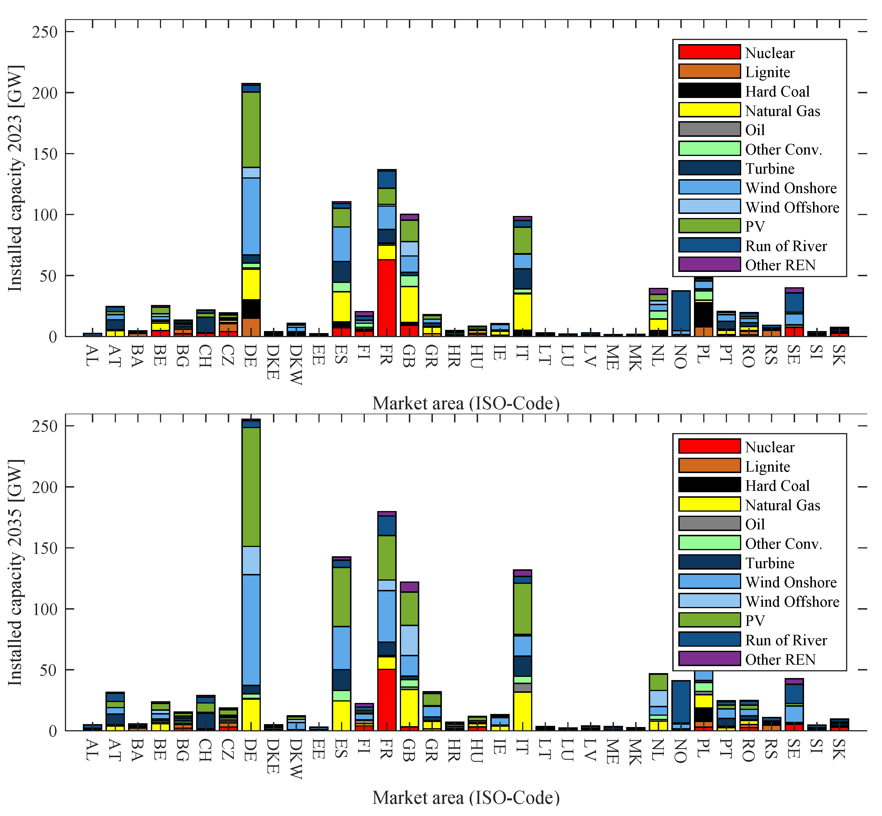The overall installed capacities per country are dis-aggregated to power plants in accordance with the Platts World Electric Power Plants Database [75]. The resulting capacities are shown in Figure 8.

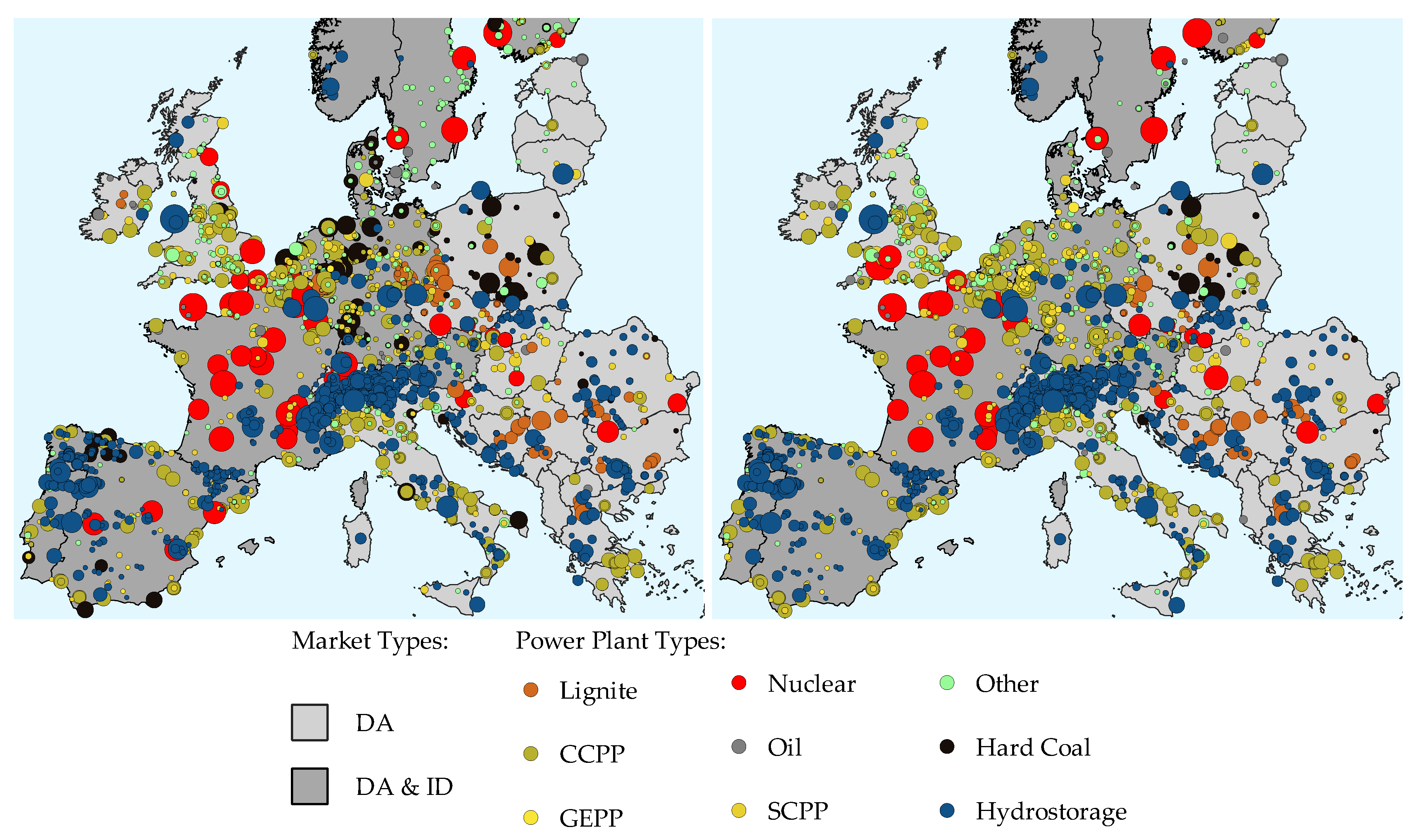
The figure shows a significant increase in installed VRE in major European countries and a decrease of conventional thermal power plants, especially coal fired plants. The regionalization of power plants for 2023 and 2035 is further depicted in Figure 9.

Historical weather data from 2012 is used to generate renewable feed-in and the European demand time series. The demand time series are taken from the ENTSO-E profiles for 2012. Moreover, the demand structure in Germany is based on [76] and the bottom-up modeling approach described in [77] in order to account for a changed load structure due to an expansion of power-to-heat systems.

The net transfer capacities between market zones are derived from [71,72,74]. AC capacities are derived by interpolation, whereas DC capacities are determined specifically for each project currently in planning. Fuel price assumptions for thermal power plants are taken from the IHS Long-Term Planning and Energy Scenarios [78], scenario “Rivalry”, except for lignite prices which are taken from [79]. $C{O}_2$-price assumptions are based on [72].

The market areas considered in this case study for ID and DA markets are depicted in Figure 9. The DA market zones are defined by the ENTSO-E areas and the ID markets by the Cross-Border ID (XBID) market areas. Maintaining the current market coupling layout (XBID) allows for a direct comparative analysis of the empirical data and the considered scenarios.

In the following, in particular, the results of the market simulations are examined from a macroeconomic perspective. The market price—as a central coordination parameter—serves as a comparative indicator for this purpose. First, the influence of the risk factors for a scenario is shown. The scenario for 2035 was selected because it includes the largest share of renewable energy and the expected effects are therefore most significant here. Subsequently, more detailed evaluations are carried out concerning the temporal characteristics of the market price and the influence of the market coupling to a fixed parameter set but for both scenarios.

6.2. Influence of Riskparameters on Optimization Results

The impact of the CVaR within the artificially emulated decision process, as outlined in Equation (16), is controlled by the quantile $\alpha$ and the risk-weighting factor $\beta$. The influence of these parameters is examined in the following subsection. Market prices represent the central coordinator between the individual power plant decisions and are therefore used as an aggregated benchmark parameter between the modeled scenarios. The risk parameter is varied by choosing $\beta \in \{0.5,1,2,5\}$ (to recapitulate Section 4, a risk parameter of 1 represents an equal weighting of the expected value and the incorporated risk). The sensitivity of the risk quantile is examined by setting $\alpha \in \{0.8,0.9\}$. A further increase of the confidence level $\alpha$ to 95% or 99% would require an increase in the number of scenarios. However, this would lead to a significant increase in computational complexity which would not be justifiable by the elbow criterion (see Section 2). In addition, the CVaR insensitive to a further increase in alpha (as shown below).

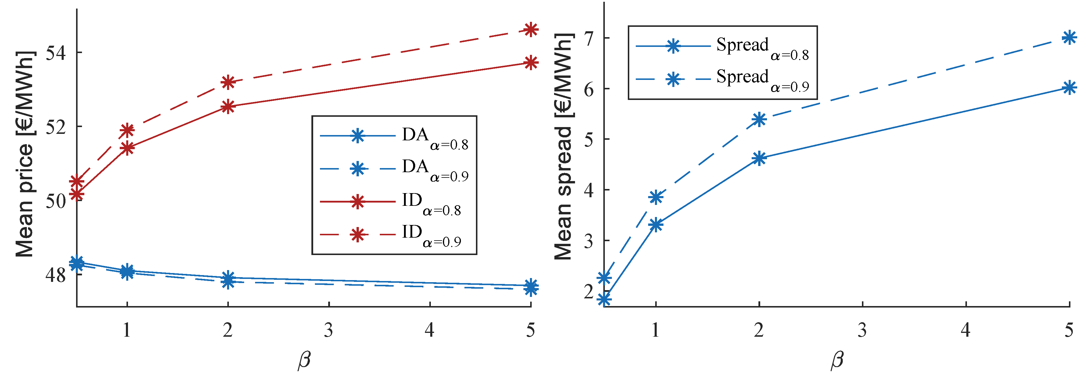
As expected, the ID price is on average higher than the DA price due to the risk aversion of the market participants (see Figure 10). Assuming a beta of 0.5, i.e., if the expected value of the objective function is weighted double as high as the risk, an ID price of 50.17 €/MWh and a DA price of 48.34 €/MWh results for $\alpha =0.8$. By shifting the CVaR quantile from 0.8 to 0.9, the ID price increases to 50.52 €/MWh, while at the same time the DA price decreases only marginally to 48.26 €/MWh. Increasing the market participant’s risk aversion by increasing $\beta$ results in a logarithmically rising average ID price. The converging spread is a plausible result. At a level of beta beyond five a further increase in risk aversion level only slightly alter the price spread because the utility function is already dominated by the CVaR expression. In addition, the stronger weighting of beta increases not only the spread between ID and DA, but also the distance between the spreads (see Figure 10 right).

It follows that the influence of the risk quantile is particularly evident when the risk is heavily weighted in the objective function. This is also plausible because risk-averse decision-makers attach greater importance to a strict risk-measure than more risk-neutral ones. In general, the resulting average market price has a higher sensitivity to the choice of $\beta$ than to the choice of $\alpha$. This result partly reflects the characteristics of the chosen risk measure CVaR. Given a certain confidence level $\alpha$ it already includes all tail elements beyond the value at risk. Conversely, taking into account only the VaR as a risk measure the choice of $\alpha$ could have a higher impact, especially based on a discrete distribution. In contrast, the variation of $\alpha$ has no influence on DA prices and the variation of $\beta$ has little influence on DA prices. The marginal price decrease in the DA market results from the transfer of cheaper generation capacity from the ID market to the DA market. The higher the contribution margin of a power plant, i.e., The lower the marginal costs of a power plant compared to the market price, the higher the risk of such a power plant on the ID market. Therefore, the ID market becomes less interesting with increasing risk weighting, especially for power plants with an average high contribution margin in the DA market. Only if the (risk-weighted) spread between the markets is significantly higher compared to the contribution margin on the certain DA market, engagement on the ID market becomes attractive. Therefore, this spread could also be interpreted as the “market price of risk”. This phenomena is also observable in real commodity markets [80]. The price spread between future quotations and expected uncertain DA prices normally incorporates a market price of risk. However, even though the average price spread between the probability weighted ID price and the DA price over an entire simulation year is positive, there are periods with negative price spreads as well. Those periods occur if there is a negative forecasting error in a major (i.e., probability weighted) part of the scenarios (a negative forecasting error is defined as a realization of more generation than forecasted.). This behavior can be derived qualitatively in the figures Figure A4.

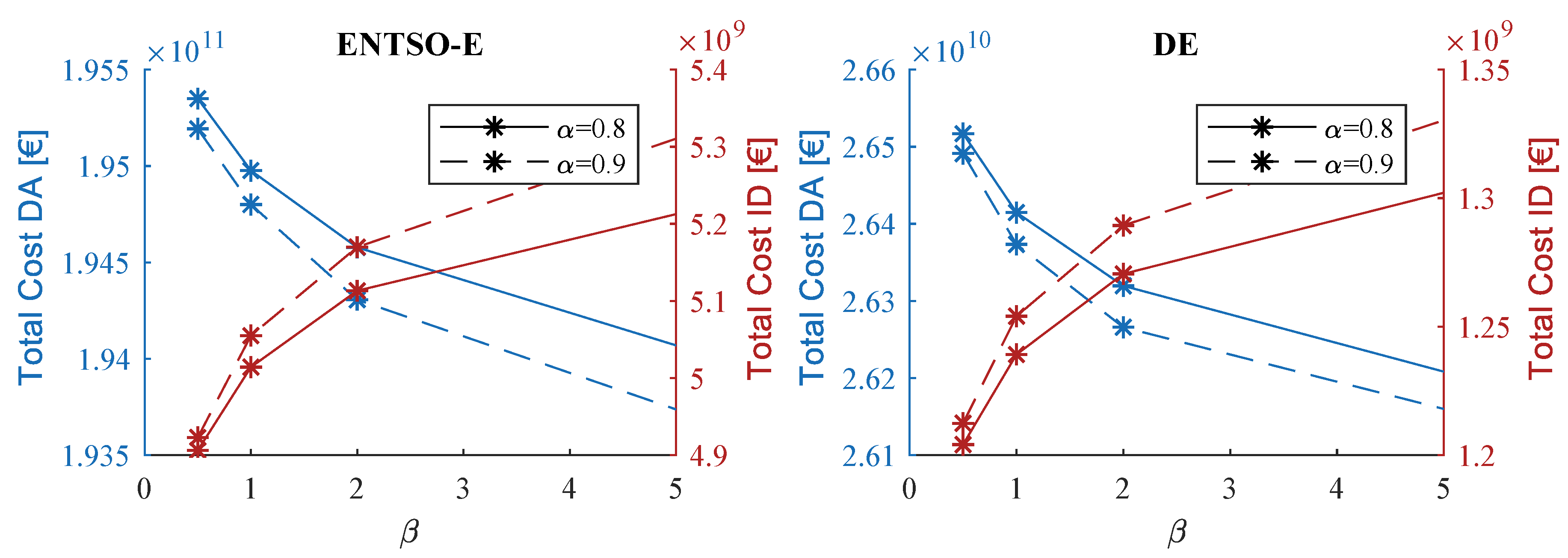
When comparing the total cost for electricity generation—both for the entire energy system (ENTSO-E) and the German market zone (see Figure 11)—the variation of the risk parameters shows a similar impact (increasing costs on ID and decreasing costs on DA when increasing $\beta$). However, while the ID costs raise by 7.3/8.5% in ENTSO-E (8.7/9.7% in DE), the DA costs only marginally decrease by 0.6/0.7% in ENTSO-E (1.2/1.4% in DE).

6.3. Derivation of Trends on the ID Market

In the following, a more detailed analysis of the optimization results for the scenario 2023 and 2035 is provided. The analysis is solely carried out for a fixed risk parameter set. This is done by setting the parameters of $\alpha =0.9$ and $\beta =1$, as this was shown to be an appropriate parametrization [81]. The comparison is based on the DA and ID market price. Afterwards, the influence of cross-border trade on the ID market is analyzed.

6.3.1. Market Price Structure

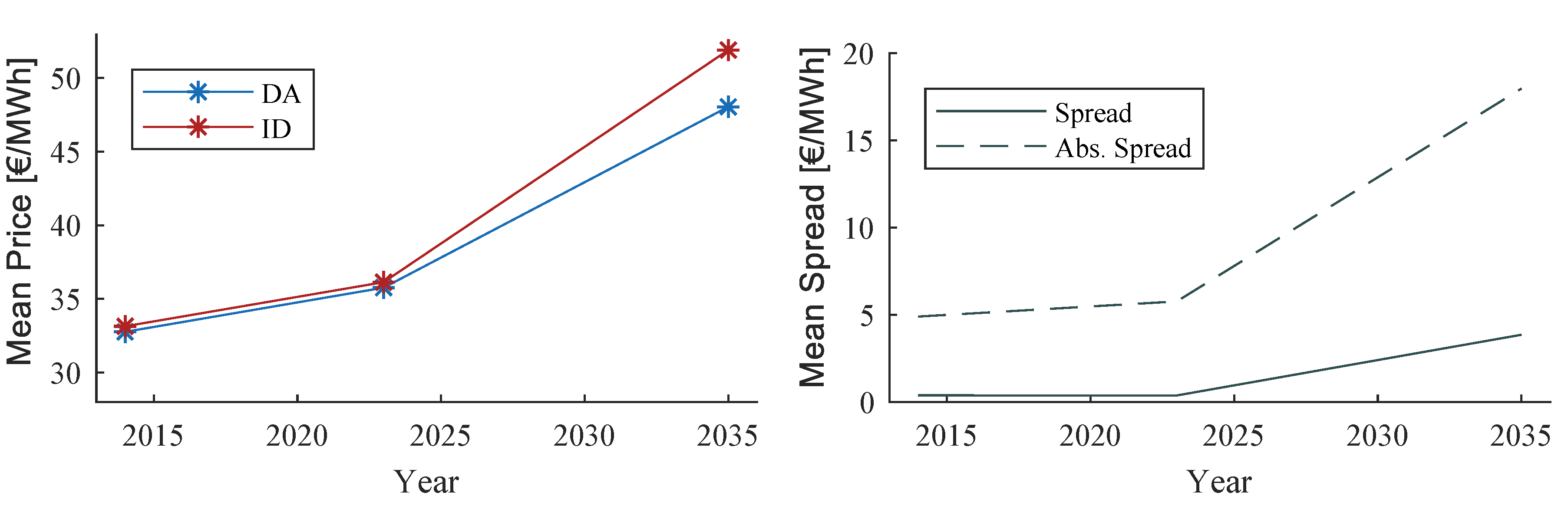
The average market price development from today over 2023 to 2035 is shown in Figure 12 for the German market area. Due to the successive decommissioning of coal-fired power plants, rising commodity- and emission allowances prices and an increasing uncertain feed-in from VRE, both a rising electricity price in general and a widening spread between DA and ID can be observed. The average DA price increases from 32.76 €/MWh (2014) via 34.82 €/MWh (2023) to 47.83 €/MWh (2035). The average ID price, however, increases from 33.14 €/MWh (2014) via 35.27 €/MWh (2023) to 51.84 €/MWh (2035). The ID price fluctuates stochastically around the DA price. Although the spread widens only marginally in the medium term from 0.38 €/MWh (2014) to 0.45 €/MWh (2023), a average positive deviation of 4.02 €/MWh is expected by 2035. In addition, the absolute spread increases according to the model from 4.90 €/MWh (2014) to 5.57 €/MWh (2023) to 17.83 €/MWh (2035). This indicates significant economic opportunities, especially for technologies that benefit from a spread in both directions.

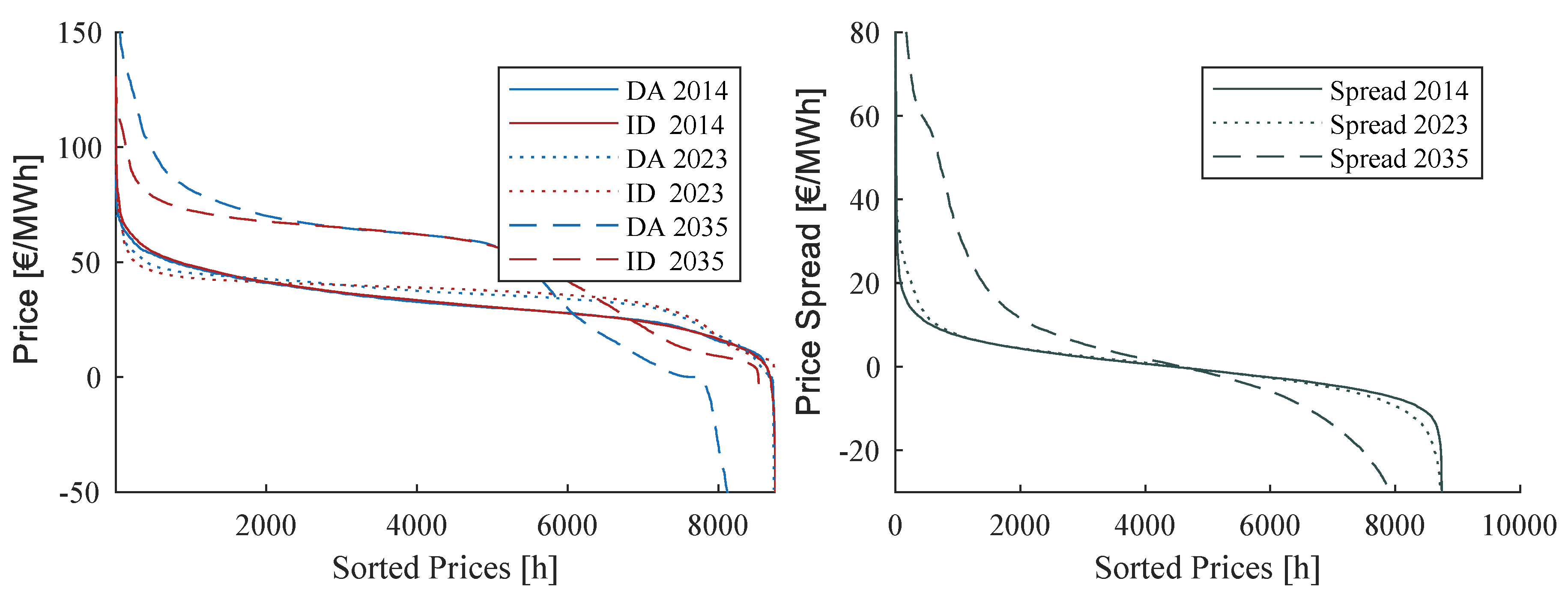
The price duration curves (PDC) of the DA and ID price resp. The price spread depicted in Figure 13. In addition to the back-test, this figure demonstrates the accuracy of the model since in 2023 the modeled spread of DA and ID prices is similar to the observed price characteristic in 2014. Moreover, it shows slightly increasing prices from 2014 to 2023 in a wide range of the PDC, with lower prices and more negative prices. The on average higher prices are due to the fact that until 2023 the phase-out of all German nuclear power plants will have taken place and thus the marginal costs of the power fleet will increase. The lower peak prices can be explained by the price dampening effect of VRE, which will have a higher share 2023. Also, the higher number in negative prices can also be explained by the rising share of VRE, which are largely subsidized by the market premium and thus have an incentive to bid their power even if the market price is negative (VRE are modeled receiving market premia ranging from 0 €/MWh to 50 €/MWh, so that they are taken off the market gradually in times of a negative residual load/negative prices). The prices for the 2035 scenario show a strong parallel shift, which is due to the, now additionally assumed, complete coal exit. This means that only gas-fired power plants with higher marginal costs remain in Germany’s thermal power plant fleet. Moreover, the assumption of a further significant increase in VRE leads to a much more volatile residual load and to more price peaks (power plant starts) and negative prices (negative residual load). Thus, the spread, as shown in Figure 13, also becomes significantly steeper, i.e., more volatile.

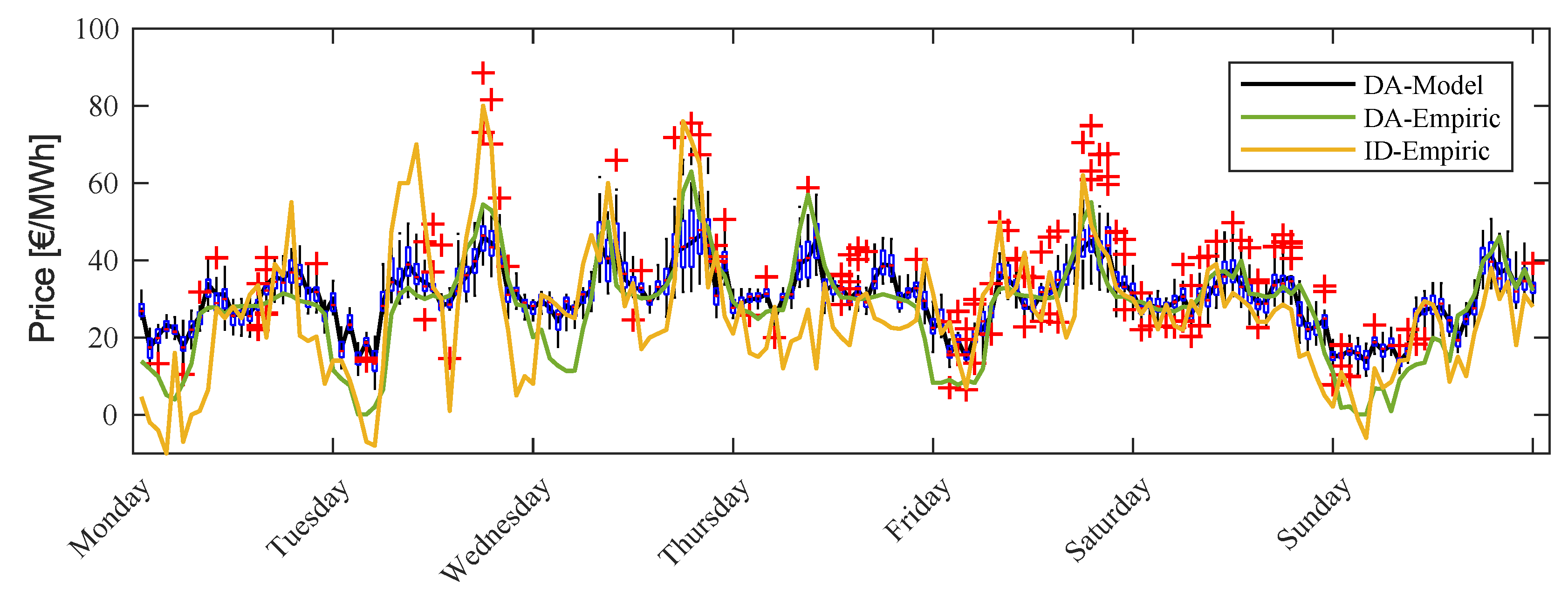
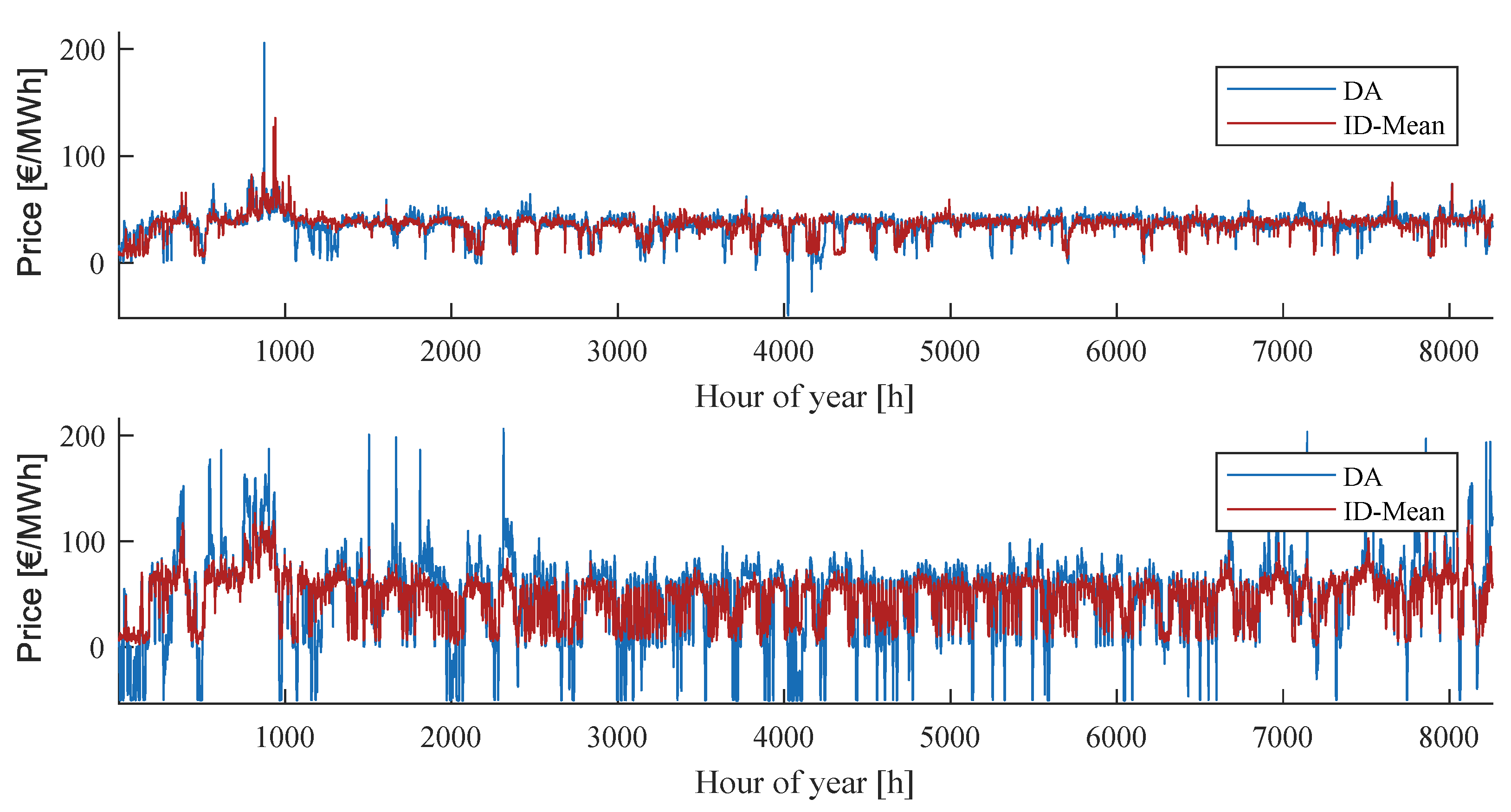
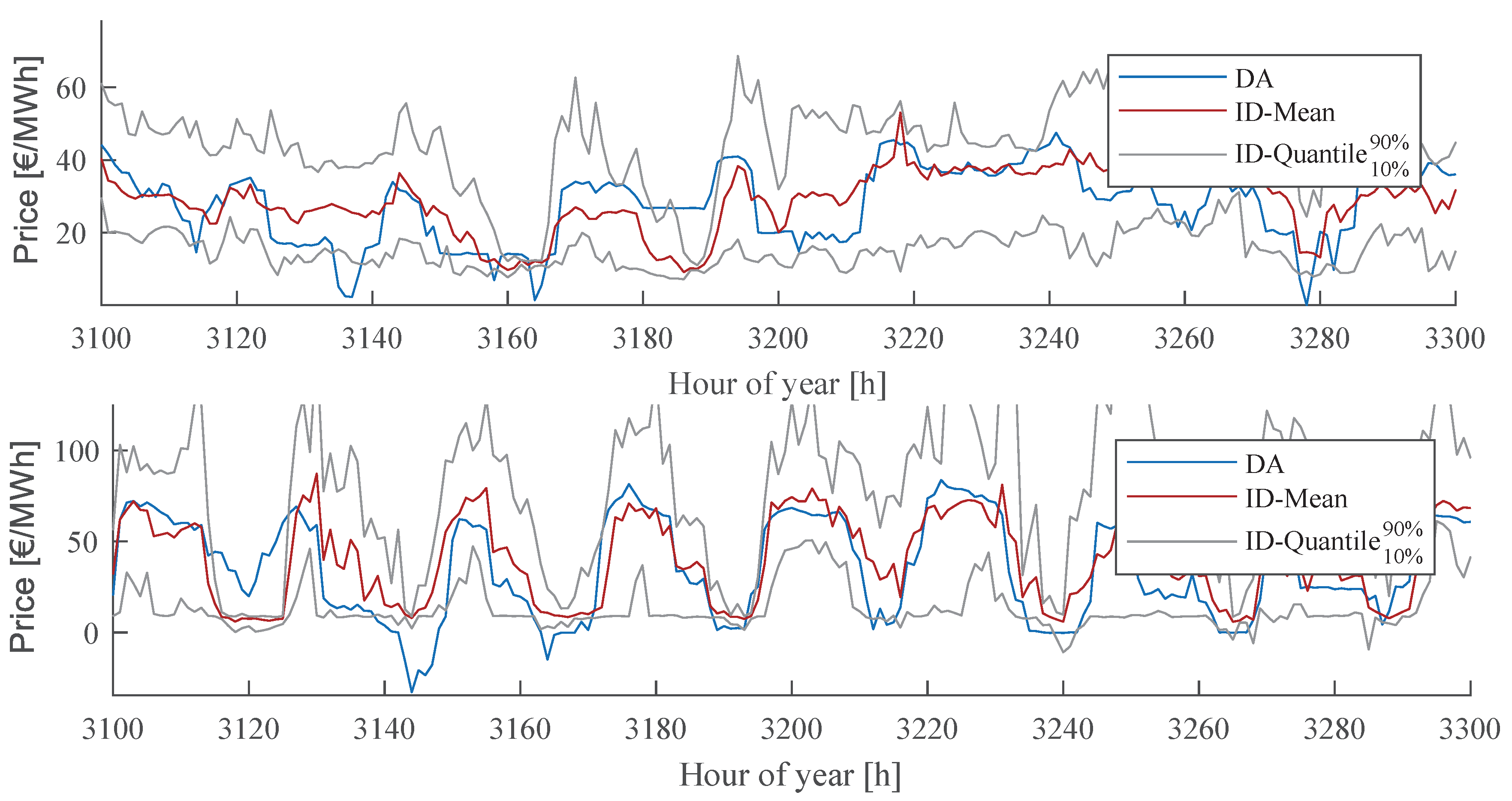
To get a qualitative impression of the dynamics of the price the time series for the electricity price in an hourly resolution for DA and ID is shown in Appendix C. Figure A3 gives an overview of the entire simulation horizon. Figure A4 shows an excerpt of the price time series from which the daily structure of the prices can be taken. In addition, the standard deviation of the ID price within each hour is depicted to better illustrate the volatility of the modeled ID prices.

6.3.2. Cross-Border Intraday Trading

The market coupling of the DA markets via EUPHEMIA was pushed forward with the aim of increasing liquidity and thus an economically more efficient allocation of resources. Following this premise, the XBID project transferred this coupling to the ID markets. In this section, we want to understand the impact of XBID on ID prices and cross-border (CB) trade through modeling the fundamental causal relationships. The scenario used is identical to the one from Section 6.3.1. An attempt was made to measure those relationships using static methods and empirical data finding a significant dependence of XBID on CB trading volumes but without a statistic dependence of XBID on ID prices resp. ID price volatility [82].

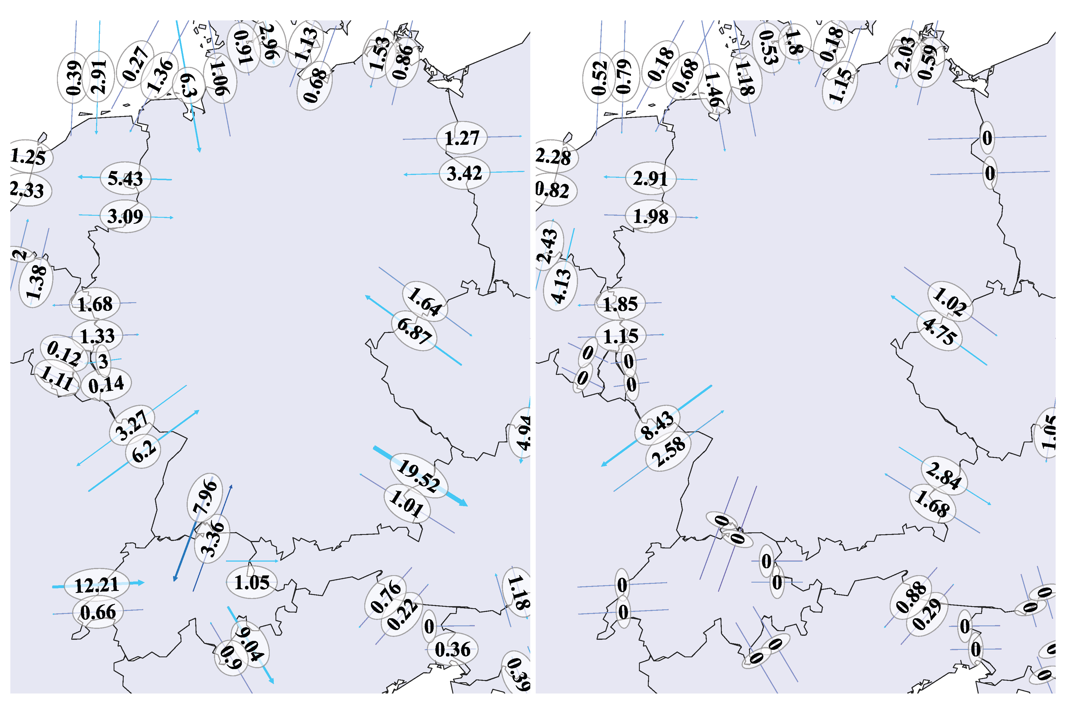
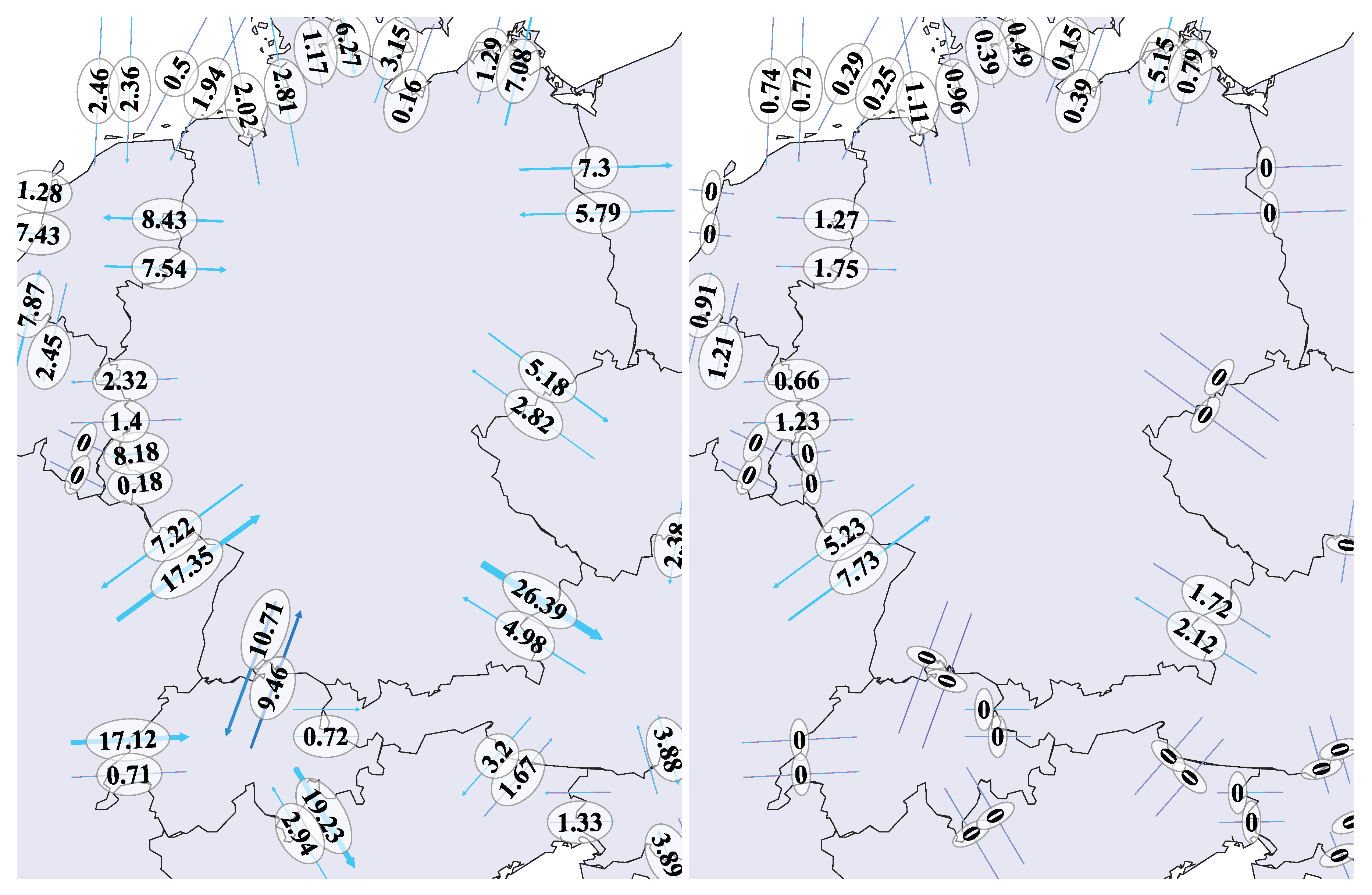
In contrast, Figure 14 shows the CB volumes of Germany and its neighboring market zones aggregated for the entire simulation year 2023. It appears that significant volumes are traded CB on the ID market especially between France and Germany (compared to the DA market). CB flows with zero values indicate non-existent couplings. Therefore, our approach is in line with the findings of [82] regarding CB trading volumes.

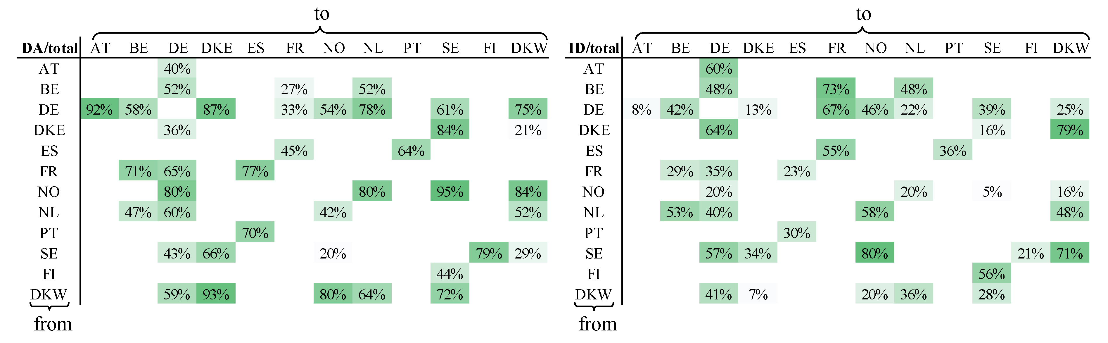
In particular, the links between DE and Scandinavia have only a minor influence on the CB volume of Germany. However, the share of the ID traded volume is particularly dominant in comparison to the DA traded volume (see Figure 15 for Scenario 2023). In principle, the relationships shown do not change over the scenarios (see Figure A5 and Figure A6 in Appendix D).

To determine the influence of XBID on market prices, the market result from above is compared to a calculation in which ID CB trading is disabled. In the analysis of [82], no statistically significant relationship between XBID and the market price was identified. However, in both scenarios, a clear influence of XBID on the price of the ID market can be measured(see

Table 2. Average price of DA and ID with and without ID CB trading (XBID) in Germany.

	2023		2035
	XBID	w/o XBID	XBID	w/o XBID
average DA Price [€/MWh]	35.83	35.91	47.83	47.30
average ID Price [€/MWh]	35.96	38.14	51.85	58.39

).

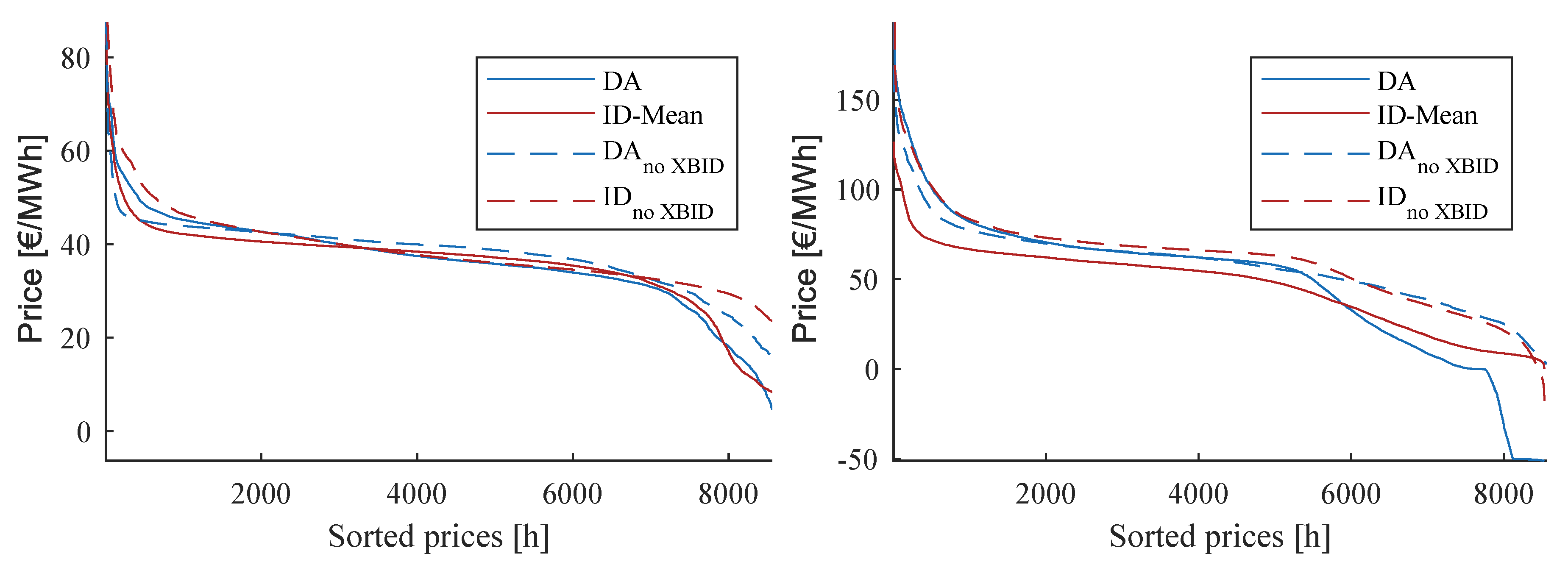
The price duration curves of this sensitivity show that the ID prices in the case with XBID are almost always (on average) below the ID prices without XBID (see Figure 16). Moreover, the spread between ID and DA without XBID is positive over the entire price duration curve, whereas in the case with XBID the spread becomes negative in a similar magnitude in high-price hours.

Due to the dominance of the DA market over the ID market, the overall economic efficiency of XBID is only marginally better in 2023. However, in 2035, when the total volume of the ID market increases due to the continuous VRE expansion, a clear increase in efficiency through XBID becomes apparent (see

Table 3. Economic benefit of CB-ID trading (spread between “w/o XBID” and “XBID”).

	Cost Spread [%]		Cost Spread [bn. €]
	2023	2035	2023	2035
DE	2.3	10.0	0.43	2.78
ENTSO-E	0.1	1.5	0.19	2.99

). With the largest absolute growth of VRE in Germany, the benefits of XBID are most evident here. Thus, this result is in distinct contrast to the empirical analysis from [82], which concludes that XBID does not influence market prices.

7. Conclusions

In this paper, we presented an unit commitment optimization model that allows the simulation of DA and ID electricity markets for large-scale energy systems. The incorporation of real decision behavior is enabled by integrating a risk measure in form of the CVaR. For this purpose, the problem is decomposed on a systemic level using Lagrangian relaxation, so that individual power plant SP can be solved independently. These Lagrangian SP are additionally decomposed with regard to their stochastic ID scenarios using Benders decomposition, which is extended by integrating cuts representing the expected second-stage recourse cost and a second set of cuts representing the second-stage CVaR.

The approach is applied to a pan-European scenario representing 2023 (considering a full nuclear phase-out in Germany) and 2035 (considering a full coal phase-out in Germany). The analyses in this paper thereby focus on the German market area. The influence of the variation in risk parameters $\alpha$ and $\beta$ was illustrated for the 2035 scenario. In that year the result is significantly influenced by the weighting of the risk $\beta$ in the objective function and less by the variation of the confidence level $\alpha$. This result demonstrates that analyses for future time periods have to incorporate uncertainty to adequately reflect the decision behavior of market participants. Given a confidence level of $\alpha =90\%$ and parity of the expected value and the risk in the objective function $\beta =1$, increasing DA and ID prices, as well as an increasing ID-DA spread, can be derived for 2023 and 2035. Finally, the influence of cross-border trading, which was extended from the DA market to the ID market within the XBID project, on trading volumes and prices was evaluated. Concerning these measures, the model is sensitive to ID market coupling.

The applied model has further development possibilities, which allow an even more detailed representation. Currently, a power plant start is only possible on the DA market. This is due to the fact that only the first stage (of the single power plant optimization problem) with the DA decision variables may include integer decision variables. The second stage, on the other hand, must fulfill the necessary condition of including only continuous variables, since otherwise no Benders cuts can be generated due to the lack of dual solutions to the optimization problem. Thus, only a power plant start stimulated by the ID market is possible, provided that this is reasonable in the expected value of the scenarios. Therefore, the power plant start in individual scenarios and consequently the ID prices in individual scenarios can be distorted. There exist approaches that approximate a dual solution in mixed-integer problems and thus enable an ID start modeling [83]. However, implementing such an approach leads to increased computational complexity. Thus, it must be assessed whether the gain in knowledge is merited by this hindrance.

Furthermore, more sources of uncertainty could be incorporated in the model (e.g., unexpected shut down of power plants or unexpected restrictions in inter-connectors or price uncertainty of ID gas prices). Lastly, different stochastic weather years and a larger simulation sample should be incorporated when future computational limits allow this.

In addition, only large-scale hydro-thermal power plants are currently simulated on the ID market. Especially distributed wind and PV power plants, which essentially dominate the trading volumes on the ID market, are not shown as active market participants. They merely offer their forecasting error on the ID market (and their forecast on the DA market). Moreover, decentralized batteries in households and the bi-directly loading of vehicles could become a potential source of flexibility in the future. Therefore, integrating the decision-making process of these power plants or rather virtual power plants that aggregate such distributed generation units into the presented approach, e.g., by [81], would be an interesting extension of the existing model.