Abstract
Due to its ability to deal with non-determinism and partial observability, represent goals as an immediate reward function and find optimal solutions, planning under uncertainty using factored Markov Decision Processes (FMDPs) has increased its importance and usage in power plants and power systems. In this paper, three different applications using this approach are described: (i) optimal dam management in hydroelectric power plants, (ii) inspection and surveillance in electric substations, and (iii) optimization of steam generation in a combined cycle power plant. For each case, the technique has demonstrated to find optimal action policies in uncertain settings, present good response and compilation times, deal with stochastic variables and be a good alternative to traditional control systems. The main contributions of this work are as follows, a methodology to approximate a decision model using machine learning techniques, and examples of how to specify and solve problems in the electric power domain in terms of a FMDP.
1. Introduction
There are planning problems in electric power plants and systems that have not been efficiently solved using traditional methods. Some of these problems have to do with the uncertain nature of the environment or the possibility of conflicts when achieving a goal. A valve can get stuck and not respond correctly to a signal from the controller, or the wheel of a forklift can skid and not have the expected position effects (uncertainty in the effects of actions). Errors in the measurement of two-phase or multiphase flow in pipes are also common (uncertainty in the state). The level in a steam drum is a variable that cannot be observed directly, it needs special instrumentation and an algorithm that estimates the level of saturated liquid contained based on the pressure and temperature in the vessel (partial observability). There are also difficulties to estimate in short-term horizons the degree of evaporation in a dam by the effect of the ambient temperature, or the amount of pluvial precipitation for a given day in a week (stochastic variables). Markov decision processes are an alternative to solve this kind of problems.
Markov Decision Processes (MDPs) [1] are a standard method for planning under uncertainty. The main advantage of MDPs is their capability to obtain a control strategy that assumes stochastic commands on actuators (uncertainty in the effects of actions). According to a preference function, MDPs optimize the expected utility. They could consider partially observable inputs and solve multiple problems using decentralized representations (multiagents). There exists some applications of MDPs reported in the literature such as power systems restoration [2], transmission system expansion [3], energy market operation [4], maintenance [5], energy resource management [6], unit commitment [7], project management and construction [8], and emergencies [9], among others. MDPs, however, require a clear representation of the state and action spaces, limiting their applicability to real-world problems. One way to address the problem of state and action explosion is through factored representations [10,11,12]. Other disadvantages of MDPs are that (i) they become difficult to solve if the problem is very complex (hundreds of state variables), in this case, abstraction or decomposition strategies might be used [13]; (ii) an adequate model of the problem is required, which can sometimes be difficult to build or approximate using machine learning; and (iii) uncertainty is not considered in the states (only in the effect of actions), fortunately the framework of partially observable MDPs [14] relaxes this limitation.
In this paper, three different planning under uncertainty applications in the electric power domain are studied: (i) optimal dam management in hydroelectric power plants, (ii) inspection and surveillance in electric substations, and (iii) optimization of steam generation in a combined cycle power plant. These problems share in common that they all are solved using the factored MDP approach. The main contributions of this paper are to (a) introduce an effective and simple learning algorithm based on decision trees and dynamic Bayesian networks to automate the factored MDP model construction, (b) emphasize the advantages and robustness of the factored MDP approach for solving planning problems in power plants and systems, and (c) provide examples of an easy problem abstraction and specification.
This paper is structured as follows. Section 2 describes MDPs, factored representations, and related machine learning methods. Section 3, Section 4 and Section 5 specify, test and discuss three applications in the electric power domain. In Section 6, some conclusions are established and future work is presented.
2. Markov Decision Processes
A Markov Decision Process or MDP [15], can be described by a tuple , in which there is a finite set of states (S), a finite set of actions (A), a probabilistic state transition function from a state and action to a probability distribution of the next state (), and a reward function ().
Two additional elements are associated with MDPs: a policy and a value function. A policy is a, possibly probabilistic, function that assigns an action for every state . A value function is the expected accumulated reward that the agent can expect to receive from a state if it follows a particular policy. It can be defined inductively, with and . There could be finite horizon or episodic models or infinite horizon models, in which case, a discounted factor (), is normally used to guarantee a bounded expected value. We can define the value function of a state in terms of other value function, as , which produces a set of linear equations in the values of .
Once an MDP is defined, the objective is to find an optimal value function which is defined in terms of an optimal policy, that satisfies, for the discounted infinite horizon case, the following equation; . The solution of this equation can be obtained using policy iteration or value iteration [15]. In policy iteration, the initial policy is selected at random and is gradually improved by finding actions in each state with higher expected value. This process continues until there is no further improvement. It has been shown that policy iteration converges to an optimal policy [15]. An alternative approach is to successively generate longer finite horizons until reaching a convergence criteria, as in value iteration. An optimal policy can be obtained over n steps , with a value function using the following recurrence association: with initial condition ∀, where is obtained from the policy as previously described. For the discounted infinite case, the optimal policy is found in a number of steps which is polynomial in , , and [15].
Given certain conditions on the rewards and transition probabilities, exists a decision rule which attains the optimal values, this implies the existence of a stationary optimal policy; so if these conditions are satisfied, there is no need for randomization [15].
2.1. Factored Markov Decision Processes
One of the problems with MDPs is that with larger and more complex problems, traditional solutions become too complex, as the space and time complexity to solve them are polynomial in terms of the number of states times the number of actions; this could become impractical for problems with large state and/or action spaces. To deal with such problems factored representations have been developed to avoid enumerating the complete domain state space, and allowing to solve more complex problems.
More formally, we can define a set of states with a set of random variables S = {}, where each variable is associated with some finite domain Dom(). A state x is defined by assigning values to each random variable ∈Dom(). As the number of state variables increases it becomes infeasible to represent explicitly the state transition model. What factored MDPs do is represent this state transition model compactly with Dynamic Bayesian Networks (DBNs) [16]. With DBNs we can represent, with small matrices, the probability distributions of the post-action nodes (at time ) given the values of their parents considering the effects of an action (see Figure 1).
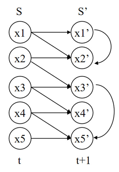
Figure 1.
A basic Dynamic Bayesian Network with 5 domain variables and diachronic and synchronic arcs.
In this representation, we can have two types of arcs: Diachronic arcs, which point from variables at time t to variables at time , and synchronic arcs, which only point between variables at time . An example of a simple DBN is shown in Figure 1, where there are five random variables (at time t and ), with nine diachronic arcs and two synchronic arcs.
A Dynamic Bayesian Network can represent the transition model with the probability distribution of the next state given a current state, following the Markov property. This is represented as a two-layered directed acyclic graph with nodes at time t and nodes at time . Each node is associated with a conditional probability distribution that specifies the probability distribution of its values given the values of its parents (): . Without synchronic arcs, the variables at time are conditionally independent of each other and the probability of each state at time can be evaluated as the product of the probabilities of the relevant variables at time .
Factored Markov Decision Processes (FMDPs) are representations that can be solved using dynamic programming which finds an optimal policy if certain conditions are satisfied, that guarantees a global optimum if it exists. Puterman [15] provides a mathematical argumentation that given an MDP model its solution is optimal. As Factored MDPs are compact representations of MDPs, this fact applies the same.
2.2. Learning Factored Models
A factored Markov Decision Process model might be approximated from data based on a random exploration in a simulated environment. We suppose that the agent can examine the state space, and that for each state–action cycle it might obtain some immediate reward. Using the data collected from this random exploration, the reward and transition functions can be learned. Given a set of N (discrete and/or continuous) random variables denoting a deterministic state, an action performed by an agent from a finite set of actions , and a reward (or cost) related to each state in an instant , we can approximate a factored MDP model [17] as follows.
- Discretize the continuous values from the original data set . This transformed sample is called the discrete data set . For not very large state spaces, use standard statistical discretization methods. In complex state spaces, abstraction methods are more efficient. For additional details see [13].
- From the subset induce a decision tree, , using the algorithm J48 [18]. This approximates the reward function in terms of the discrete domain variables, .
- Order the data such that the attributes follow a temporal causal ordering, e.g., before , before , and so on. The set of attributes should have the following structure , .
- Prepare the data set for the induction of a set of 2-stage dynamic Bayesian networks, splitting the data into subsets of samples, one subset for each action.
- Learn a transition model for each action using the K2 algorithm [19]. The result is a 2-stage dynamic Bayesian network for each action .
The resulting factored MDP model is solved using dynamic programming to obtain the optimal policy. There exists several software tools for solving these representations [20,21]. The methodology presented is applied to three different problems in the electric power domain.
3. Optimal Dam Management in Hydroelectric Power Plants
The development of operation policies for dam management [22,23,24] is a difficult and time-consuming task that requires multidisciplinary expert knowledge. A special challenge is how to manage the inherent uncertainty of the rain behaviour in order to optimize the level of water of the storage containers, and at the same time keep the dam at a safe state while satisfying the energy demand. Water resources planning activities respond to the opportunities to obtain increased benefits from the use of water and related resources. However, the intermittent nature and the uncertainty of these water resources make them hard to solve. Traditionally, Geographic Information Systems (GIS) have been built for resource planning and design studies. In [25], the authors compare some of these tools in the context of small scale hydropower resources. For the dams and reservoirs optimal operation, more powerful stochastic methods of computational intelligence are required [26].
We propose an approach for the problem of creating optimal operation policies for an hydroelectric system. The system is composed of the following elements: (i) a reservoir; (ii) an inflow conduit, regulated by , which can be either a spillway from another dam or a river; and (iii) two outflow spillways: , which is connected to the turbine and thus generates electricity, and , allowing direct water outflow without electricity generation. Consequently, the reservoir has two inflows coming either from the inflow conduit or the rainfall, and two outflows. We quantify all flows to a flow unit L, and consider them as multiples of this unit. We include four discrete reservoir levels: MinOperL, MaxOperL, MaxExtL, and Top, and consider the transition between the different levels.
The unit, L, is the amount of water that is required to move from one level in the reservoir to another, and it is defined by
where is a unit of flow, is the surface of the reservoir, and is a unit of time. Thus, the rainfall, , the inflow, and the outflows are multiples of L,
where is the inflow at , and are the outflows at , and and . The rainfall is classified as follows,
The objective of the optimization is to control , , and so that that the water volume in the reservoir is at the optimum level as close as possible, MaxOperL, given the rainfall conditions. This optimization process helps to find the optimal conditions of operation of the hydroelectrical system, and suggest the best decisions according to the meteorological and hydrological conditions.
To model four interconnected dams, four copies of the previous single dam model are connected. This set-up is depicted in Figure 2, it is a more complex problem, so the decision system has to consider the inflows and outflows of each dam; the rainfall, that can be vary between dams, given there different locations; additionally, it is required to define the operation policies of each one to maintain them as close as possible to the MaxOperL level.
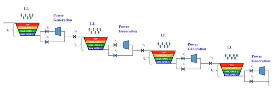
Figure 2.
Multiple dam system.
The consequences of an incorrect decision in the operation of each dam might impact not only a particular dam but all the dams in the system.
3.1. MDP Problem Specification
The specification of a factored MDP requires the definition of (i) the set of states, (ii) the set of actions, (iii) the reward function, and (iv) the state transition functions. We consider a simplified version of the state space including the state variables: rain intensity (Rain) and dam level (Level). Rain can have three different values: Null, Moderate, and Heavy; Level can have eight different values: MinOperL1, MinOperL2, MaxOperL1, MaxOperL2, MaxExtL1, MaxExtL2, Top1, and Top2. Thus, the total number of state is x . The actions correspond to the permitted operations on the control elements (valves or gates): , and . For this case, we include the actions to open or close a valve or a gate.
The definition of the reward function considers: positive reward for the dam levels near the MaxOperL value, and negative reward for the levels near the top limits. The reward is independent of the rainfall intensity. Figure 3 depicts a decision tree of the reward as a function of the dam levels.
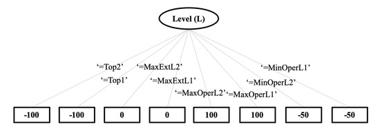
Figure 3.
The reward function is represented as a decision tree. Dam levels of MaxOperL1 or MaxOperL2 are rewarded 100 economic units (best case). MaxExtL1 or MaxExtL2 levels receive a reward of 0 (irrelevant). Top1 or Top2 levels are penalized by −100 (worst case). Level MinOperL receives a reward of −50 (bad).
Figure 4 depicts the transition model for action under three different scenarios. In all of them, the dam level is set to the MaxOperL level (red mark on interval 3–4). In the first column, the Rain variable is instantiated to Null (blue mark in interval 1). In this case, the dam level has no change. Level_1 is maintained in the interval 3–4 (orange mark). In the second scenario (second column), the Rain variable takes the value Moderate (interval 1–2), so that the level increases to reach the interval 4–5 with 80% of probability. Finally, in the last scenario (third column), Rain is heavy (interval 2–3), and as a consequence, with 80% of probability, the dam level increments to the interval 5–6. The last column shows the structure of the two-stage dynamic Bayesian network (DBN) representing the transition model for action .
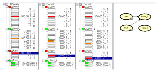
Figure 4.
Transition model for action under three different rainfall scenarios (): null (column 1), moderate (column 2), and heavy (column 3). Last column shows the structure of the dynamic Bayesian network for this action. The model and scenarios are shown using Hugin [27].
3.2. Experimental Results
Using the problem specification for the hydroelectric domain, we solved the corresponding factored MDP to find an optimal action policy. The different policy effects on the dam level are illustrated in Table 1. As example, the effect of the actions Close_, Close_, and Close_ means that the effect on the level is null because the recommended action will maintain the level, given that the rain has no impact on the system. In case of experiencing a low dam level, and independently of the rain condition, the policy will recommend the actions Open_, Close_, and Close_, which increase the dam level ↑. In this case, the rain could increase the level in one or two steps depending on the rain intensity. In the opposite case, when the dam level is high, the effect of the actions Close_, Open_, and Open_ will decrease the dam level as a function of the rain magnitude.

Table 1.
Effects of the policy on the dam level (L) depending on the rain condition ().
In order to demonstrate the effects of the policy in the system, we tracked the optimal policy starting from a random initial state to the goal state, under two scenarios: one-dam system and four-dam system. In this simulation, we generated the next states according to the transition function, considering as the next state that with the highest probability.
In the first scenario, the dam was set to the minimum operation level (level = MinOperL) and with no rain (rain = Null). The optimal policy was executed during 20 steps (time-horizon) to observe the utility behavior. Figure 5 (left) illustrates how the dam initiates with an expected utility of 427.68 units, in the next step the system reaches a utility value of 588.30 units, and in the third step it achieves the maximum utility of 771.23 units.
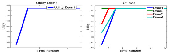
Figure 5.
(left) Utility values for a one-dam system. (right) Utility values for a four-dam system.
In a second scenario, we started with multiple dams at the conditions illustrated in Table 2. In order to check an optimal behavior, twenty steps were simulated. As shown in Figure 5 (right), the (blue line), which was initiated with a low level, achieved the value considered as optimum in three steps. The (green line) started in an optimal or goal state and remained in the same state. The (red line), which initiated with a max extraordinary level, reached the maximum utility value in only two state transitions. Finally, the (light blue line) that was started with a high dam level got the optimal value in three steps.
Table 2.
Initial states (Level (L) and Rainfall ()) and utility values for a four-dam system.
The specified model applies for each dam in isolation. Assuming that the dams have the same characteristics in capacity and that they are located in the same area, the model is fully reusable. Otherwise there would be variations in the model parameters and intervals of the variables. Specifying a model for the dam system in a coordinated manner requires powerful abstraction techniques and supercomputing to deal with the resulting complexity.
3.3. Discussion
Solutions based on physical models like those used in [25] are difficult to build and require longer solution times than factored MDPs. On the other hand, the restoration time is a key issue to minimize the effects of a natural phenomena and avoid economic and human loses. FMDPs provide a rapid restoration time for dams.
The potential use of the shark algorithm is presented in [26] as an optimization algorithm used for single reservoir and for multi-reservoir optimal operations. This algorithm is a stochastic search optimization method that generates an initial set of random potential solutions, from which it selects the best interactively. A weakness with this technique is its vulnerability to be trapped in local optimum. Factored MDPs solutions, on the other hand, guarantee a global optimum, allow to deal with stochastic variables such as Rainfall, and could solve multiple dam systems in a multiagent framework (Decentralized factored MDPs).
4. Inspection and Surveillance in Electric Substations
Substations are facilities located often at remote places so that their inspection, surveillance, and maintenance are complex tasks. Some of the typical activities for the inspection of remote substations are related to fault detection of primary substation equipment such as power interrupters, instrument transformers, power transformers, sectioning switches, and surge arrestors. Typical failures are usually caused by environmental agents or deficient maintenance tasks. In a substation there are high-tension regions and high-temperature components that must be considered as risky zones and interest zones, respectively. Interest components might be collector bars, cooling oil tanks, or transformer windings.
The problem of equipment inspection and surveillance in electric substations has been attacked using mobile robots with capabilities of visual object detection, path planning, visual localization and obstacle detection, positioning, and localization and control [28,29,30].
In this work we use a mobile robot provided with navigation sensors, high voltage testers, and thermal and infrared cameras to inspect a substation installation. This robot must optimize the use of its resources while avoiding risky zones and reaching inspection goals safely. This is why, navigating reliably with autonomy and rationality is always required, although is too a challenging task (Figure 6).
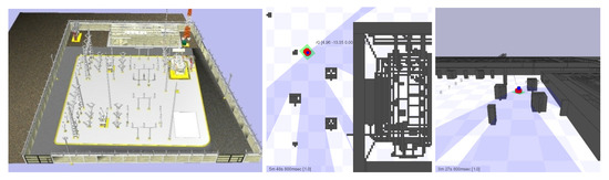
Figure 6.
Virtual scaled environment. (left) 3D substation model. (center) 2D robot approaching the power transformer. (right) 2.5D robot approaching the power transformer.
4.1. MDP Problem Specification
Given that autonomous navigation in outdoors can be stated as a planning problem with multiple goals immerse in an uncertain world, one proper framework for this is based on factored Markov Decision Processes. For this FMDP specification, states are physical locations in the substation area (Figure 7) (left), and the possible actions are orthogonal movements of a mobile robot to the right (R), left (L), up (U), or down (D). Risky zones (−100, −30), inspection areas (10), and other interest points (1) are associated to a reward function that will lead the robot throughout convenient navigation paths (Figure 7) (center). The remaining zones can be assigned with a neutral reward (0).

Figure 7.
(left) Two robots in a simulated navigation area. (center) Reward function. (right) Optimal navigation policy.
The inspection system must be able to distinguish objects with elevated and normal temperature as well as risky zones. In Figure 7 (center), red cells represents risky zones (points with elevated tension) and the blue cells represents points under normal tension. Green cells are locations with normal tension and a great surveillance perspective. When the mobile robot detects a blue or a green cell it has to stop and send information to the central system to notify, from a safe place, the condition of a particular equipment (high/normal temperature). Yellow cells are less risky zones than red cells. Green cells, on the contrary, represent very safe zones with a high concentration of equipment susceptible to failure.
4.2. Experimental Results
To evaluate its behavior, this problem was implemented in a simulated navigation environment using the Player Stage tool [31]. The resulting policy, shown in Figure 7 (right), drives the robot to secure areas (blue and green cells) while preventing the robot from falling into risky zones (red and yellow cells). The utility-time graph shown in Figure 8 demonstrates that the utility for the robot increases progressively and it is steady when the robot achieves the inspection area. For a time step of 2 s, the maximum expected utility is achieved in 88 s (44 steps).
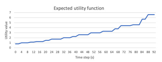
Figure 8.
Utility function for a robot using a factored Markov Decision Processes (FMDP) controller.
The policy for rotating movements is also shown in the topological map of Figure 9. Rotating movements are go_forward →, right_turn ⥁, left_turn ⥀, and the null_action. In this new setting, inspection areas are assigned with positive immediate reward (300), and risky zones with negative reward (−300). In order to simulate real motion, a 10% of Gaussian noise can be added to the robot actuators. The method, that was tested using the SPI tool [21], successfully guides the robot to positions with higher rewards. For instance, assuming that the robot has a discrete orientation s2 at the position (s3, s2), the optimal policy commands the robot to turn right ⥁ until it gets orientation s1 and turn right ⥁ again to get orientation s0. In this new state, the policy indicates the robot to go forward → and achieve the inspection position (s4,s2) with reward = 300.
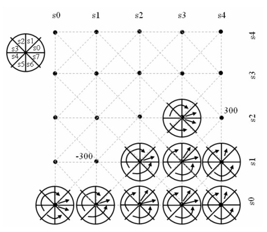
Figure 9.
Resulting policy on an discrete topological map for rotating movements.
Table 3 shows some data related to the evaluation of the processes of learning and inference of factored MDPs for a selected set of experiments of different complexities. Particularly, the number of samples collected in the exploration, learning and inference time, and the size of the state space. The first row of the table shows the results from experiments with the rotating robot. The following rows correspond to experiments with orthogonal movements. In all these experiments, a discount factor of 0.9 was used.
Table 3.
Experimental results of learning and inferring factored MDPs.
The learning times of a factored model vary from 2033 s. for a problem with 64 states, up to 11,697 s. for cases with 900 states. This shows that the learning method is a reasonably quick process that can be considered treatable. On the other hand, it was observed that as the number of samples was increased, the optimal policy is approached, and the value also improved. The solution times of the model with value iteration are standard and depend on both the number of states listed as the processor used in the test. These times vary between 20 ms. and 9.73 s.
Finally, and with the aim to reduce the dimensionality of the problem, we compared factored MDPs versus the approach of qualitative MDPs [13], which combines abstraction and refinement of the state-space. Table 4 shows the results of four different state partitions and reward values. As it can be seen, substantial time reductions can be achieved under different conditions.
Table 4.
Comparison of abstraction-refinement methods versus a discrete factored MDP under different problem configurations.
4.3. Discussion
Focusing on the path planning aspect utilized in related applications, there are significant efforts in trying to solve the navigation problem in substations. In [32], for example, the algorithm and a re-tracking method based on Dynamic Window Approach (DWA) are used to perform the obstacle avoidance and path planning. The problem with the DWA is that, as a local reactive method, in many cases, there is no guarantee that the robot will reach the goal position. It may get stuck in local minima.
In [33], the authors describe an autonomous mobile robot which can interact and plan its motion in an unknown environment based on the information acquired using nine infrared sensors. The obstacle avoidance and goal reaching algorithms proposed are based on fuzzy logic. The obstacle avoidance and goal reaching controllers are connected to a wavelet network-based motion controller through a mobile robot kinematic model to obtain a complete autonomous mobile robot system. In contrast with FMDPs, fuzzy logic systems are not always accurate, it is difficult to acquire and define rules to determine the membership function parameters, and there is no guarantee of optimal solutions.
FMDPs guarantee a global optimum, depending on the size of the discretization, FMDPs can offer more accurate results, and FMDP models can be learned using data applying machine learning techniques.
5. Optimization of Steam Generation in a Combined Cycle Power Plant
In complex processes like power plants, one of the crucial requirements in its operation is to deal with a great amount of information that can be used for the decision-making process. For example, under abnormal or unusual situations, an operator needs to select the relevant information to rapidly identify the source of the problem, and effectively define the decisions or action plan to take the process into safe conditions. Under these conditions, an intelligent system that can assist the operator and provide some support functions becomes a relevant aid. Some of these auxiliary tools are reported in literature. For example, the authors of [34] propose an advisory system to assist operators of a nuclear power plant. The proposed system can detect, validate, diagnose, mitigate, monitor, and recover from faults. More in the direction of aids for power plant control, the authors of [35] state the use of a genetic algorithm to determine optimum operating parameters of the boiler unit as the basis for improving a power plant performance.
In general, two main trends have been followed in modern power plants: (i) leave very few decisions to the operator with high instrumentation and automatization and (ii) operate the plants close to their limits. Nevertheless, the skills and experience of the operators are still required in some maneuvers. For instance, in a steam generation system it is common to have an electric load disturbance. In a combined cycle power plant, the gas turbine is responsible of generating electricity and additional electricity can be generated with the waste heat using a steam turbine. The steam generation system has different components. In order to recover residual energy, the heat recovery steam generator (HRSG) takes the exhaust gases of the gas turbine and uses them to heat water (see Figure 10). A mixture of steam and water is produced from the HRSG (Ffw) which goes through the feedwater valve (fwv) to the steam drum. The steam drum is responsible of separating this mixture and ensure a dry steam flow to the steam engine. The main steam valve (msv) regulates this steam flow. The residual water is extracted from the steam drum by the recirculation pump to supply water into the HRSG. This process produces a steam flow with high pressure (Fms) that goes into the steam turbine to produce electric energy (g).
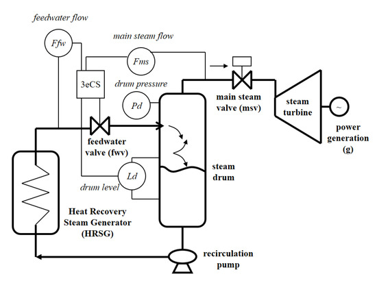
Figure 10.
Main components of the steam generation system. The connection to the gas turbine is not shown.
A state transition can be induced by an electric load disturbance (d). Given this exogenous event, we have to design a control strategy on the valves that maximizes the security in the drum or in the power generation, considering a preference function.
5.1. MDP Problem Specification
The steam generator operation variables can be used to directly define the set of states of a factored MDP. Namely, as controlled variables, the main steam flow (), the feedwater flow (), the power generation (g), and the drum pressure (), and, as uncertain exogenous event, the disturbances (d). The state of the plant is represented by a combination of the possible values of these variables which are previously discretized in a small set of intervals.
The optimal operation of a plant is normally defined by recommended operation curves that express the relation that certain state variables must satisfy. For instance, Figure 11 shows the recommended operation curve between the drum pressure and the main steam flow. These curves can be used to define a reward function for an MDP. States that follow the curve are assigned positive rewards while, the rest of the states are given negative rewards. As soon as the MDP is fully defined for the plant, an optimal policy can be obtained to maintain the plant in its optimal operation curve.
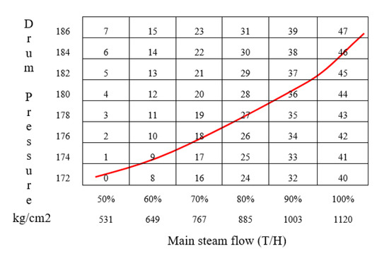
Figure 11.
Recommended operation curve for a Heat Recovery Steam Generator.
In this example, the set of actions consist of opening and closing the feedwater () and main steam valves (), which regulate the feedwater flow and the main steam flow, respectively. We denote, () and (), as the actions to open and close , and () and (), as the actions to open and close . No changes in the valves are denoted by the null action ().
In the example, the state variables were discretized in the following values (shown in parenthesis): , , (2), , and , so the state dimension space is . A two-stage Bayesian network [16] is used to represent the state transition model (see Figure 12). Solid lines represent direct effects over the next state variables when applying a particular action, while dashed lines represent that the next state variables are not affected by that action. The action effects are denoted in this work by , , and for the null action.
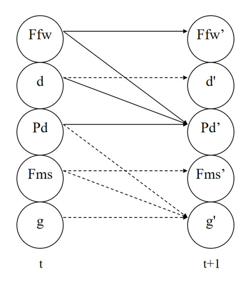
Figure 12.
A two-stage Dynamic Bayesian Network for the steam generation system. The solid lines represent the effects for actions and and the dashed lines the effects for actions and .
Following this approach, it is easy to construct a transition model. We just need to identify, for each action, the state variables and those affected by the action. For instance, for actions and , we need to enumerate the possible states of , d and () and those affected by these actions ( possibilities). Therefore, we do not need to enumerate all the domain variables at time t (evidence variables) or at time (interest variables). Additional savings can be obtained when we specify the reward function, since we only need to specify a reward value for the characteristic states, in this case, and .
5.2. Experimental Results
We tested the factored MPD model in a combined cycle power plant simulator that allows different settings. In particular, it can include states with sudden disturbances (see Chapter 12 [36]). An interface is also provided to see how fast the recommendations from the system transforms an abnormal state into a secure and optimal operation. The experiment consisted of whether or not different operators followed the policy to (i) to optimize the process or (ii) treat a disturbance. During the test, the plant was operated in manual mode and under three different load scenarios: full load (30 MW), medium load (20 MW), and minimum load (15 MW). Figure 13 shows the average of utility for a medium load case to optimize the process. When the operators follow the recommended action (green and blue lines matching), the utility (red line) increases. Otherwise, the utility might decrease or in the best case remains the same.
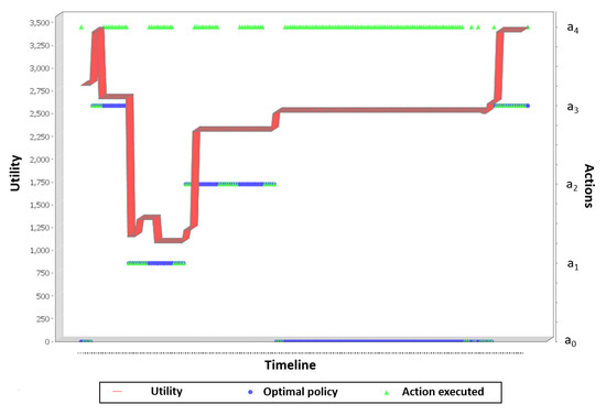
Figure 13.
Utility plot for a plant running at medium load (20 MW). When the operator operator executes the recommended actions , or the utility increases. When the operator does not follow the recommended action and instead applies , the utility remains the same. In other cases, when the operator does not follow the recommended action, the utility decreases.
We solved the same problem by adding two extra variables, the position for valves and , and using nine actions (all the combinations of open-close valves and ). We also redefined the reward function to maximize power generation, g, under safe conditions in the steam drum. Although the problem increased significantly in complexity, the policy obtained is “smoother” than the 5-action simple version presented above. To give an idea about the computational effort, for a fine discretization (15,200 discrete states) this problem was solved in 859.2350 s, while using a more abstract representation (40 discrete states) it took 14.2970 s.
The importance of applying this method in the optimization of a steam generator and from the operation point of view is that a power plant could safely restore from a disturbance with a minimum number of actions, producing time savings and significant risk reductions.
5.3. Discussion
The computerized operator support system (COSS) presented in [34] for using in a Generic Pressurized Water Reactor (GPWR) included a recommender module that monitored multiple sets of sensor data and provided early warnings of emerging system faults (e.g., rapidly lowering level). Given that it is not clear how the recommender system interacts with alarms, procedures and process and instrumentation diagrams (P&IDs) to direct operators to actions, it is assumed that there is not an optimization or intelligent criteria for action selection, and consequently there are not optimal recommended actions. FMDPs provide optimal action policies based on the model.
The main idea in [35] was to determine the thermodynamically optimum size or operating regime of steam boiler using genetic algorithms with a real power plant as a case study. Genetic algorithms have the advantage that they do not require a complete system model and can be employed to globally search for the optimal solution. The disadvantage is that they do not guarantee to find a globally optimal solution. Among other drawbacks are its convergence time, difficulties to fine tune their parameters, and that their solutions are difficult to interpret. FMDPs guarantee (if there exists) an optimum solution and they can be solved effectively.
6. Conclusions
In this paper, three different planning under uncertainty applications in the electric power domain solved with FMDPs were shown. The main contributions of this work are (i) an alternative to specify and solve planning problems under uncertainty in the electric power domain and (ii) a methodology to approximate a decision model using machine learning techniques.
The main results of the FMDP approach for each application might be expressed in terms of operation improvements, efficiency, and robustness:
- Optimal dam management in hydroelectric power plants. Good compilation times and rapid restoration time of hydroelectrical systems. They allow to deal with stochastic variables such as Rainfall. Because factored MDPs find global solutions, it is possible that by using a more abstract approach and restricting system exploration to review only possible states (exclusion of unlikely states), models can be built to manage the operation of multiple dams simultaneously.
- Inspection and surveillance in electric substations. FMDPs guarantee a global optimal path. Depending on the size of the discretization, they can offer accurate results, and good compilation and response times. The relative ease of designing reward functions in this domain prevents inspection robots from causing or having accidents at the facility, thus avoiding economic losses or damage to nearby areas. It is possible to find an optimal or at least suboptimal policy even in the event of possible errors in the execution of the actions of a robot (e.g., tire skidding or jamming). Factored MDPs allow an inspection robot to navigate reliably in outdoor settings (uncertain environments), at the same time that it provides autonomy, rationality and task organization.
- Optimization of steam generation in a combined cycle power plant: (i) it provides optimal action policies (recommendations), (ii) it guarantees a globally optimal solution, (iii) it has good compilation times, and (iv) it is a good alternative to traditional control systems. In cases of load disturbances, such as load rejections, where the steam generator requires quick response, damage to turbines, electric generators and other devices is avoided. FMDPs considers that the valve actuators may not respond exactly to the control system (uncertainty in the effects of the actions), it also considers the utility of the steam generator states through an immediate reward function. Traditional control methods does not consider the uncertainty in the water level sensing in the steam drum, which can be solved using partially observable FMDPs.
These techniques can also be successfully applied to similar domains. For instance, either in the power industry or petroleum industry, there are a number of different chemical processes that are difficult to control because of the uncertainty in actuators and because their states cannot be observed directly. Among them, we could mention: oil refinement, water treatment, cooling systems, and oil production. In electric power systems, the electrical distribution is another problem that could be effectively solved using FMDPs.
As future work, we would like to extend the methodology to divide large problems of the electric power domain into sub-problems that can be solved more efficiently by using a decentralized factored MDP.
Author Contributions
Conceptualization, L.E.S., A.R., and E.F.M.; software, A.R. and P.H.I.; investigation, A.R. and P.H.I.; writing—original draft preparation, A.R.; writing—review and editing, L.E.S., P.H.I., and E.F.M.; project administration, A.R. and L.E.S.; funding acquisition, A.R. and L.E.S. All authors have read and agreed to the published version of the manuscript.
Funding
This research was funded by the National Institute of Electricity and Clean Energy (INEEL)—Mexico project number 14716B, the Portuguese Fundaçao para a Ciência e Tecnologia (FCT) project number 73266, and the FONCICYT project number 95185 (CONACYT-EU).
Acknowledgments
The authors thank the publication sponsors through Project FORDECyT No. 296737 “Consortium in Artificial Intelligence” and students and collaborators for their participation in the systems development.
Conflicts of Interest
The authors declare no conflict of interest.
References
- Bellman, R. Dynamic Programming; Princeton U. Press: Princeton, NJ, USA, 1957. [Google Scholar]
- Ghorbani, J.; Choudhry, M.A.; Feliachi, A. A MAS learning framework for power distribution system restoration. In Proceedings of the Transmission and Distribution Conference and Exposition, Chicago, IL, USA, 14–17 April 2014. [Google Scholar]
- Dusonchet, Y.P.; El-Abiad, A. Transmission Planning Using Discrete Dynamic Optimizing. IEEE Trans. Power Apparatus Syst. 1973, PAS-92, 1358–1371. [Google Scholar] [CrossRef]
- Löhndorf, N.; Minner, S. Optimal day-ahead trading and storage of renewable energies—An approximate dynamic programming approach. Energy Syst. 2010, 1, 61–77. [Google Scholar] [CrossRef]
- Chen, D.; Trivedi, K.S. Optimization for condition-based maintenance with semi-Markov decision process. Reliab. Eng. Syst. Saf. 2005, 90, 25–29. [Google Scholar] [CrossRef]
- Liu, Y.; Yuen, C.; Hassan, N.U.; Huang, S.; Yu, R.; Xie, S. Electricity Cost Minimization for a Microgrid With Distributed Energy Resource Under Different Information Availability. IEEE Trans. Ind. Electron. 2014, 62, 2571–2583. [Google Scholar] [CrossRef]
- Nikovski, D.; Zhang, W. Factored Markov decision process models for stochastic unit commitment. In Proceedings of the 2010 IEEE Conference on Innovative Technologies for an Efficient and Reliable Electricity Supply, Waltham, MA, USA, 27–29 September 2010. [Google Scholar]
- Manjia, M.B.; Kedang, V.F.; Kimbembe, P.L.; Pettang, C. A decision support tool for cost mastering in urban self-construction: The case of Cameroon. Open Constr. Build. Technol. J. 2010, 4, 17–28. [Google Scholar] [CrossRef][Green Version]
- Zhou, L.; Wu, X.; Xu, Z.; Fujita, H. Emergency decision making for natural disasters: An overview. Int. J. Disaster Risk Reduct. 2018, 27, 567–576. [Google Scholar] [CrossRef]
- Boutilier, C.; Dean, T.; Hanks, S. Decision-Theoretic planning: Structural assumptions and computational leverage. J. AI Res. 1999, 11, 1–94. [Google Scholar] [CrossRef]
- Boutilier, C.; Dearden, R.; Goldszmidt, M. Stochastic dynamic programming with factored representations. Artif. Intell. 2000, 121, 49–107. [Google Scholar] [CrossRef]
- Patrascu, R.; Poupart, P.; Schuurmans, D.; Boutilier, C.; Guestrin, C. Greedy linear value approximation for factored Markov decision processes. In Proceedings of the Eighteenth AAAI/IAAI National Conference on Artificial intelligence, Edmonton, AB, Canada, 28 July–1 August 2002. [Google Scholar]
- Reyes, A.; Sucar, L.E.; Morales, E.; Ibarguengoytia, P.H. Abstraction and Refinement for Solving Markov Decision Processes. In Workshop on Probabilistic Graphical Models PGM06; Citeseer: Prague, Czech Republic, 2006; pp. 263–270. [Google Scholar]
- Kaelbling, L.P.; Littman, M.L.; Cassandra, A.R. Planning and acting in partially observable stochastic domains. Artif. Intell. 1998, 101, 99–134. [Google Scholar] [CrossRef]
- Puterman, M. Markov Decision Processes; Wiley: New York, NY, USA, 1994. [Google Scholar]
- Darwiche, A.; Goldszmidt, M. Action networks: A framework for reasoning about actions and change under understanding. In Uncertainty Proceedings; Morgan Kaufmann: Burlington, MA, USA, 1994; pp. 136–144. [Google Scholar]
- Reyes, A.; Spaan, M.T.J.; Sucar, L.E. An Intelligent Assistant for Power Plants Based on Factored MDPs. In Proceedings of the 15th Intl. Conf. on Intelligent System Applications to Power Systems, Curitiba, Brazil, 8–12 November 2009. [Google Scholar]
- Quinlan, J. C4.5: Programs for Machine Learning; Morgan Kaufmann: San Francisco, CA, USA, 1993. [Google Scholar]
- Cooper, G.F.; Herskovits, E. A bayesian method for the induction of probabilistic networks from data. Mach. Learn. 1992, 9, 309–347. [Google Scholar] [CrossRef]
- Chadès, I.; Chapron, G.; Cros, M.J.; Garcia, F.; Sabbadin, R. MDPtoolbox: A multi-platform toolbox to solve stochastic dynamic programming problems. Ecography 2014, 37, 916–920. [Google Scholar] [CrossRef]
- Reyes, A.; Ibarguengoytia, P.H.; Santamaría, G. SPI: A Software Tool for Planning under Uncertainty based on Learning Factored Markov Decision Processes. In Advances in Soft Computing; Lecture Notes in Computer Science Series; Springer: New York, NY, USA, 2019; Volume 11835. [Google Scholar]
- Abdel-hameed, M.; Nakhi, Y. Optimal control of a finite dam using policies and penalty cost: Total discounted and long run average cases. J. Appl. Probab. 1990, 27, 888–898. [Google Scholar] [CrossRef]
- Abramov, V.M. Optimal Control of a Large Dam. J. Appl. Probab. 2007, 44, 249–258. [Google Scholar] [CrossRef][Green Version]
- McInnes, D.; Miller, B. Optimal control of time-inhomogeneous Markov chains with application to dam management. In Proceedings of the 2013 Australian Control Conference, Fremantle, Australia, 4–5 November 2013; pp. 230–237. [Google Scholar]
- Punys, P.; Dumbrauskas, A.; Kvaraciejus, A.; Vyciene, G. Tools for Small Hydropower Plant Resource Planning and Development: A Review of Technology and Applications. Energies 2011, 4, 1258–1277. [Google Scholar] [CrossRef]
- Ehteram, M.; Karami, H.; Mousavia, S.F.; El-Shafie, A.; Amini, Z. Optimizing dam and reservoirs operation based model utilizing shark algorithm approach. Knowl.-Based Syst. 2017, 122, 26–38. [Google Scholar] [CrossRef]
- Andersen, S.K.; Olesen, K.G.; Jensen, F.V.; Jensen, F. Hugin: A shell for building Bayesian belief universes for expert systems. In Proceedings of the Eleventh International Joint Conference on Artificial Intelligence, Detroit, MI, USA, 20–25 August 1989; pp. 1080–1085. [Google Scholar]
- Jian, Y.; Xin, W.; Xue, Z.; ZhenYou, D. Cloud computing and visual attention based object detection for power substation surveillance robots. In Proceedings of the 2015 IEEE 28th Canadian Conference on Electrical and Computer Engineering (CCECE), Halifax, NS, Canada, 3–6 May 2015. [Google Scholar]
- Wu, H.; Wu, Y.X.; Liu, C.A.; Yang, G.T. Visual data driven approach for metric localization in substation. Chin. J. Electron. 2015, 24, 795–801. [Google Scholar] [CrossRef]
- Xiao, P.; Yu, L.X.; Chen, S.H.; Wang, H.P.; Wang, B.H. Design of a laser navigation system for substation inspection robot based on map matching. Appl. Mech. Mater. 2015, 713, 713–715. [Google Scholar] [CrossRef]
- Vaughan, R.T. Massively multi-robot simulations in Stage. Swarm Intell. 2008, 2, 189–208. [Google Scholar] [CrossRef]
- Zhou, M.L.; He, S.B. Research of autonomous navigation strategy for an outdoor mobile robot. Int. J. Control Autom. 2014, 12, 353–362. [Google Scholar] [CrossRef]
- Hamzah, M.I.; Abdall, T.Y. Mobile robot navigation using fuzzy logic and wavelet network. IAES Int. J. Robot. Autom. (IJRA) 2014, 3, 191–200. [Google Scholar] [CrossRef]
- Boring, R.L.; Thomas, K.D.; Ulrich, T.A.; Lew, R.T. Computerized Operator Support Systems to Aid Decision Making in Nuclear Power Plants. Procedia Manuf. 2015, 3, 5261–5268. [Google Scholar] [CrossRef]
- Egeonu, D.; Oluah, C.; Okolo, P.; Njoku, H. Thermodynamic Optimization of Steam Boiler Parameter Using Genetic Algorithm. Innov. Syst. Des. Eng. J. 2015, 6, 53–73. [Google Scholar]
- Sucar, L. Decision Theory Models for Applications in Artificial Intelligence: Concepts and Solutions; Premier Reference Source, Information Science Reference; IGI Global: Pennsylvania, PA, USA, 2011. [Google Scholar]


© 2020 by the authors. Licensee MDPI, Basel, Switzerland. This article is an open access article distributed under the terms and conditions of the Creative Commons Attribution (CC BY) license (http://creativecommons.org/licenses/by/4.0/).