Optimization of a Small Wind Turbine for a Rural Area: A Case Study of Deniliquin, New South Wales, Australia

Abstract

The performance of a wind turbine is affected by wind conditions and blade shape. This study aimed to optimize the performance of a 20 kW horizontal-axis wind turbine (HAWT) under local wind conditions at Deniliquin, New South Wales, Australia. Ansys Fluent (version 18.2, Canonsburg, PA, USA) was used to investigate the aerodynamic performance of the HAWT. The effects of four Reynolds-averaged Navier–Stokes turbulence models on predicting the flows under separation condition were examined. The transition SST model had the best agreement with the NREL CER data. Then, the aerodynamic shape of the rotor was optimized to maximize the annual energy production (AEP) in the Deniliquin region. Statistical wind analysis was applied to define the Weibull function and scale parameters which were 2.096 and 5.042 m/s, respectively. The HARP_Opt (National Renewable Energy Laboratory, Golden, CO, USA) was enhanced with design variables concerning the shape of the blade, rated rotational speed, and pitch angle. The pitch angle remained at 0° while the rising wind speed improved rotor speed to 148.4482 rpm at rated speed. This optimization improved the AEP rate by 9.068% when compared to the original NREL design.

1. Introduction

Energy demands are increasing worldwide and exponentially, given the rising population and needs for economic growth [1]. Consumption of energy is expected to increase by 56% from 553 quadrillion kJ to 855 quadrillion kJ for the period 2010 to 2040 [2]. The extensive consumption of fossil fuels is the primary source of CO₂ emissions into the atmosphere, which is estimated to increase from 31 to 36 billion metric tons during 2010–2020 and may reach 45 billion metric tons by 2040 [3]. The demand for what is termed “clean energy” has increased enormously in recent years due to the fact of people’s environmental awareness, desire for energy security, and governments enacting increasingly strict environmental policies [4]. Of all the renewable energy sources, wind energy seems to be favored due to the fact of its low price and rapid global development [5]. The global power installation from wind energy rose from 296,581 MW in 2013 to 539,291 MW in 2017, and it is predicted to reach 817 GW by 2021 [3].

Location has a significant effect on the power output of wind turbines. Accounting for environmental conditions when designing the HWAT for a specific area or region could improve the power output. Many researchers have optimized the rotor shape of wind turbines to maximize the annual energy output. Optimization of the wind turbine blade shape was undertaken at Gökçeada [6] in Turkey using different blade design parameters, i.e., twist angle and chord length. The results showed that the highest AEP of 92,972 kW-hr was comparable to the combined experiment rotor (CER) test of the National Renewable Energy Laboratory (NREL) with the original design. Darwish et al. [7] improved the AEP for low wind speed regions by selecting, laying out, and matching the most suitable wind turbine system for a case study conducted in Iraq. Liu et al. [8] demonstrated a novel optimal blade design method for the twist angle and chord length radial profiles of a fixed-pitch, fixed-speed wind turbine which performed excellently with lower manufacturing costs. Blade element momentum (BEM) theory helped to design the rotor diameter, nominal speed ratio, and the tip speed ratio of a 300 kW HAWT based on wind speed data in Semnan, Iran [9].

Blade element momentum theory and computational fluid dynamics (CFD) are the most popular methods for estimating the performance and aerodynamic characteristics of wind turbines. Plaza et al. [10] analyzed the aerodynamic performance of a New Mexico wind turbine rotor using the k-ω SST model and compared the results with that of BEM. At low wind speeds, the BEM model achieved better results than the k-ω SST CFD model. However, at high wind speeds, BEM failed in separating the flow conditions when a detachment occurred in the blade. The inaccuracy was due to the three-dimensional effects and blade tip losses. Conversely, CFD agreed well with the experimental data over a wide range of wind speeds.

The literature is abundant with various CFD computation models. For example, Li et al. [11] investigated NREL Phase VI using unsteady Reynolds-averaged Navier–Stokes (RANS) and detached eddy simulation (DES) models. The study found that the RANS results of thrust forces and moments differed from the experimental work. The DES generated considerable improvements in the unsteady flow of wind turbines. Lanzafame et al. [12] and Rajvanshi et al. [13] simulated NREL Phase VI using k-ω SST and transitional k-ω. The results demonstrated that transitional k-ω agreed better with experimental data than k-ω SST. Moshfeghi et al. [14] investigated the effects of near-wall grid treatment on the aerodynamic performance of a wind turbine. The thrust forces results of k-ω SST for eight different cases did not agree well with the test results. In general, the k-ω SST model over-predicted the performance of the wind turbine. Transitional k-ω, on the other hand, confirmed better prediction accuracy and particularly in the inboard regions.

Until now, there was no unique model that could predict all the physical characteristics of turbulent flows. The k-ε turbulence models were used to study the flow around the wind turbine and wake dynamic behavior. Kasmi and Masson [15] and AbdelSalam and Ramalingam [16] executed a full-scale study of three wind turbines based on different k-ε turbulence models and compared results with experimental work. Their findings confirmed that the modified k-ε agreed better with previous experimental measurements than standard k-ε. Abdelsalam et al. [17] simulated the upstream and downstream velocities for a 2 MW HAWT using a modified k-ε turbulence model which showed good agreement between measured and predicted results. Siddiqui et al. [18] studied the dynamic wake behavior of an NREL 5 MW wind turbine with two different approaches, i.e., multiple reference frame (MRF) and sliding mesh interface (SMI). They found that SMI had a better prediction ability near the hub than MRF. However, SMI required a tremendous amount of computational resources to deliver fully converged results. Rütten et al. [19] computed the NREL Phase VI using k-ω and k-ω SST using Open-FOAM code. Their findings revealed that the k-ω model overestimated the turbulent kinetic energy when compared to the k-ω SST turbulence model.

The CFD modelling has been widely used to investigate aerodynamic characteristics concerning the wind turbine. In the present work, the aerodynamic characteristics of a 20 kW wind turbine were investigated using four RANS models including k-ω SST, transition SST, Spalart–Allmaras, and realizable k-ε. In addition, the NREL test results of mechanical torque and blade pressure distribution were used for model validation. Depending on this numerical validation, the best performing CFD model will be used to examine the mechanical output with different rotational speeds and variable pitch angle, so that the optimized blade design can be compared. Location has a significant effect on the wind turbines’ power output. Accounting for the environmental conditions when designing the HWAT for a specific area or region could improve the power output. Research has focused on the aerodynamic optimization of the shape of the wind turbine; this is critical in the manufacturing and design of the wind turbine. Australia has widespread and plentifully distributed wind resources. There is a lack of research about the design of wind turbines that takes into account the prevailing environmental conditions in Australia. This study aims to optimize a 20 kW wind turbine for the rural region at Deniliquin, New South Wales, using the horizontal axis rotor performance optimization (HARP_Opt) code. This paper optimized the wind turbine shape to maximize AEP, depending on the Weibull distribution function. The present study is structured as follows. Section 2 and Section 3 present the numerical modelling and optimization methods, respectively. Section 4 discusses the simulation results, and Section 5 summarizes and concludes the critical findings of this study.

2. Numerical Modeling of HAWT Under Separation Conditions

2.1. Governing Equations of Selected Turbulence Models

The principle of the mathematical concept of the RANS equations is based on the calculation method of the Navier–Stokes equation which is divided into the instantaneous fluctuating part and the average flow part. In the present work, the aerodynamics of the wind turbine is predicted with a commercial CFD code known as Ansys Fluent 18.2 [20]. The flow around a wind turbine blade is considered to be incompressible and is modelled utilizing the RANS method. The software uses the finite volume method for solving the mass and momentum equations in addition to equations of turbulence for each control volume cell. The mass and momentum conservation equations are:

$$\frac{d{\overline{u}}_i}{dx}=0$$

(1)

$$\frac{\partial {\overline{u}}_i}{\partial t}+\frac{\partial }{\partial x_j} \left({\overline{u}}_i {\overline{u}}_j\right)=-\frac{1}{\rho } \frac{\partial \overline{p}}{\partial x_i}+v \frac{{\partial }^2{\overline{u}}_i}{\partial x_j\partial x_j}-\frac{\partial }{\partial x_j} \left(\overline{{\acute{u}}_i {\acute{u}}_j}\right)$$

(2)

where ${\acute{u}}_i$ is the fluctuating velocity, ${\overline{u}}_i$ the mean velocity, and $v$ the fluid kinematic viscosity.

The realizable k-ε [21], k-ω SST [22], Spalart–Allmaras [23], and transition SST [24] models are the four RANS models which were investigated. The governing equations of the four RANS models are described in Appendix A.

This section of the paper aims to investigate the effect of those four turbulence models on predicting the aerodynamic characteristics of the twisted wind turbine where the mechanical torque and blade pressure distribution are used for model validation when compared with the NREL test results. Secondly, the differences among the turbulence models under different wind speeds that include stall conditions are documented through simulation of the wind turbine.

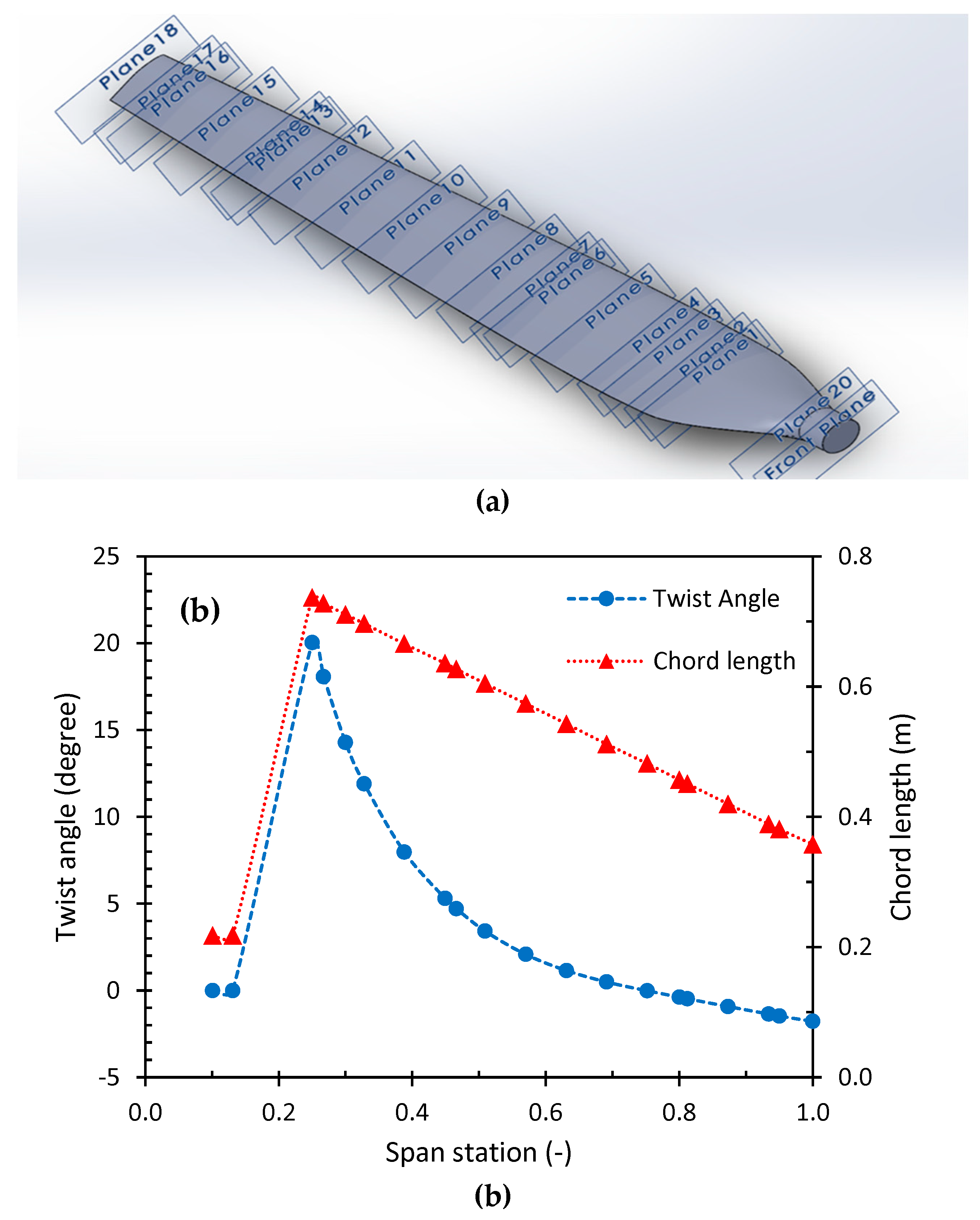
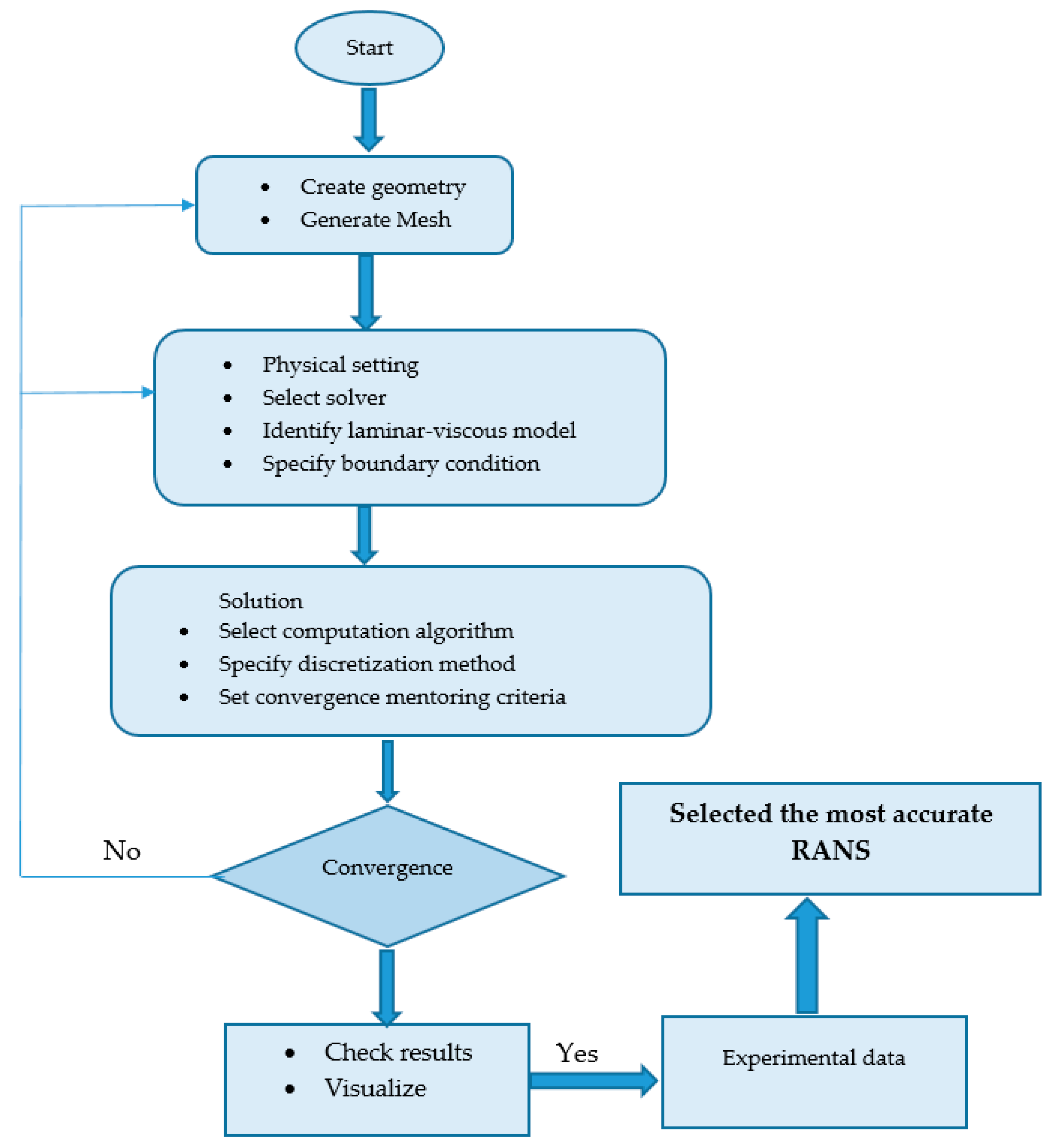
2.2. CFD of Wind Turbine

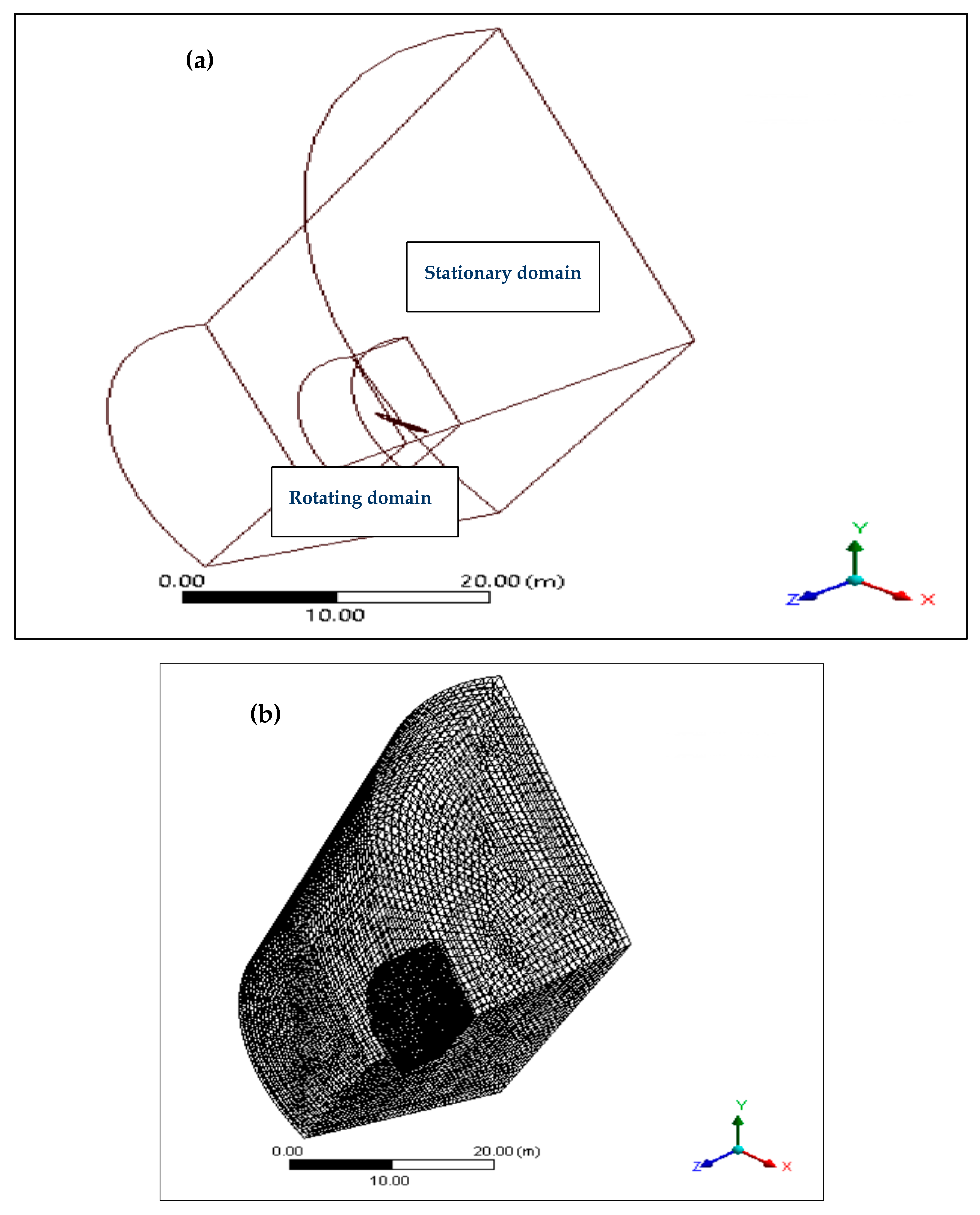
2.2.1. Computational Domain

The NREL (CER) extends the NREL (VI) experiment rotor [25] which was performed in the National Renewable Energy Laboratory. The geometry of the 20 kW wind turbine blade was optimized to maximize the annual energy [26]. The results explained the prediction complexity of the aerodynamic performance of the tapered-twisted HAWT turbine when compared with an untwisted blade. As such, the NREL CER performs excellently compared to the commercial blades. The NREL CER was used as a reference for validating the aerodynamic performance of a three-blade wind turbine with variable speed operations.

Table 1. Specification and operating parameters of the NREL CER.

Parameters	Value
Rated power	20 kW
Blade diameter	10.58 m
Number of blades	3 blades
Hub height	12.192 m
Pitch angle	5°
Rotational direction	Counterclockwise
Rotational speed	72 rpm
Power regulation	Stall regulation

summarizes the main characteristics of the wind turbine blade with S809 airfoil applied from a 25% span at the root to the tip.

The blade geometry was created using SolidWorks [27] and disregarded the effect of the tower and nacelle to reduce computational time and enhance numerical stability [28]. The wind blade consisted of 18 sections as shown in Figure 1a. These sections had different twist angles and chord lengths along the blade as shown in Figure 1b. The geometry of the cylindrical part ended at 0.66 m from the axis of rotation and then started to change until the transition area ended at 1.25 m. From Figure 1b, the maximum twist angle reached 20.040° at 0.25 span and later became zero at a 0.75 span and a negative value at a 1.00 span.

The fluid domain was divided into two zones as shown in Figure 2a. The first zone with a 120° radial stream tube was generated with periodic faces to decrease computational time due to the symmetrical flow around the wind turbine model. The upstream velocity was specified with an 18 m radius, offset 12 m in front of the blade. Meanwhile, the downstream outlet was defined with a 36 m radius, offset 24 m behind the blade, and specified as an atmospheric pressure outlet. The second zone was near the blade with a 10 m radius and 5 m from the center of the root. This zone was created to separate the rotating and stationary zones and to increase the number of mesh cells near the blade. The upstream velocity and upper surface of the domain were specified as free stream wind speed. This conical shape of the domain was used to permit wake conical expansion on the back of the blade. An important step is choosing the most suitable computational domain. First of all, a proper computational domain that permits rotation of the wind turbine blade with a no-slip wall effect is essential when considering the optimization of mesh quality. Consequently, a large computational domain will not permit enough grid generation around the wind turbine. On the other hand, a vast domain would increase the computational time corresponding with an increase in the calculated number of cells.

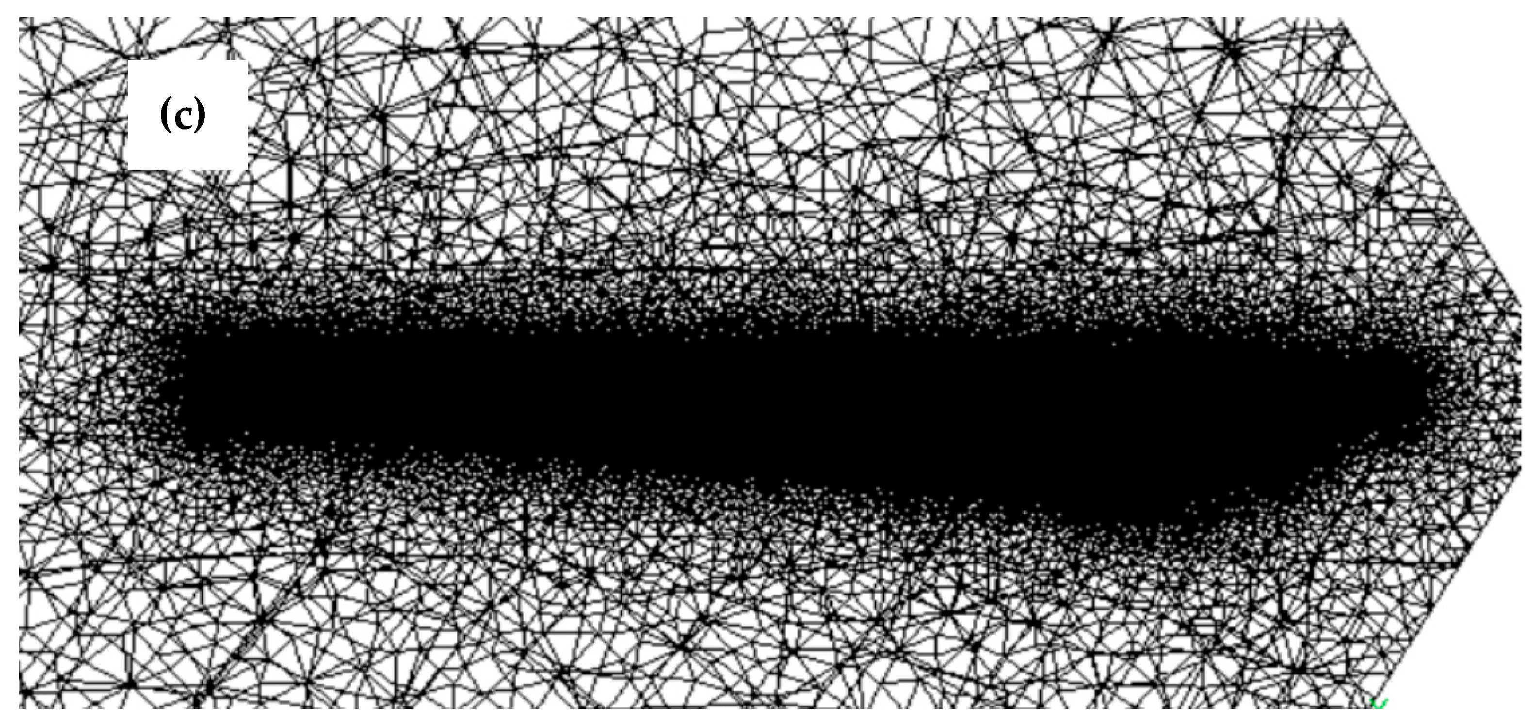
2.2.2. Computational Mesh Generation

The S809 airfoil has a very sharp trailing edge along the blade which produces non-orthogonal face cells [29]. These cells lead to low-quality mesh and inaccurate or unstable CFD solutions. Generating a sharp trailing edge is not possible in the experimental work, so rounding this sharp edge through a radius of 1 mm will improve the quality of the mesh with an insignificant effect on the CFD results.

The present study used different turbulence models to predict the output power and pressure distribution under a variety of wind speed conditions which was crucial to refining the mesh around the blade rotor. As shown in Figure 2b, the cells were refined gradually away from the blade to reduce the computational time. The ANSYS meshing was used to generate unstructured mesh, and a local and global sizing was used to produce a high-quality grid. The minimum mesh size was 0.008 m³ around the blade. After that, inflation was used to refine the prismatic cells at the blade surface, and it generated fifteen prismatic layers with a growth rate of 1.2 as shown in Figure 2c.

Also, he proximity and curvature with the fine relevance center were defined as the specification of the local mesh size function which helped to refine the mesh grid. Mesh quality plays a crucial role in the accuracy of CFD results. However, a smaller mesh size requires a longer computation time and more computer memory. For this reason, it is essential to compromise between accuracy and computational time. On the other hand, it is crucial to achieve mesh independence. Nine meshes were tested at a 7.2 m/s wind speed to achieve grid independence by monitoring the mechanical torque. As shown in Figure 3, the CFD results converged when the number of mesh cells was 3,559,082, which had an error rate of 3.82% when compared with the measurement value. Any further increase in the number of mesh cells will significantly raise the computational time but will lead to no improvement in the accuracy. For this reason, 3,559,082 mesh cells is deemed to be the most suitable mesh configuration in terms of computational time and efficiency.

Three models are used in ANSYS Fluent for handling the rotational effect, namely, dynamic mesh, sliding mesh, and moving reference frame (MRF) models. The sliding mesh model is appropriate for the transient flow problem but requires a full-scale model. Both dynamic mesh and sliding mesh models require high computational resources. The MRF model is the simplest way for modelling the flow of steady-state rotating objects without using rotating mesh to reduce the computational time [30]. Thus, MRF is applied in the small zone near the blade to apply the rotational speed of the wind turbine with periodic boundary conditions. The transformation from a stationary to a moving frame in terms of relative fluid particle velocities, Coriolis, and centripetal accelerations have been used to calculate the MRF model. The MRF was set-up for computation domain by applying a rotational speed of 72 rpm with the absolute reference frame. The blade was assumed to be a non-slip stationary wall that had a zero-relative velocity with other adjacent cells.

2.2.3. Numerical Method and Boundary Conditions

Four turbulence models were used to predict wind turbine aerodynamics. All regions in the domain were applied to the boundary conditions. Domain outlet was applied to the pressure boundary conditions of zero gauges pressure with 101,325 Pa of atmospheric conditions. The current investigation focused on 15 inlet velocities ranging from 4.9m/s to 15.2 m/s which was enough to investigate the prediction of different turbulence models for stall delay phenomena. The air density waas approximately constant due to the assumption of incompressible fluid [11]. In this study, the standard air properties were used, where air density and dynamic viscosity were 1.225 kg/s and 1.7894 × 10⁻⁵ kg/ms⁻¹, respectively.

The steady-state, pressure-based method was used to solve the incompressible RANS models. A semi-implicit method was used to model the velocity and pressure in momentum and continuity equations. The convergence rate is improved when using a combined algorithm rather than a simple algorithm.

The first-order upwind was used for solving turbulent kinetic energy and the turbulent dissipation rate, while a second-order upwind scheme was used for solving the momentum equations. The least squares cell-based method was used in a gradient spatial discretization scheme. A standard discretization scheme was used in the pressure values interpolation.

In the simulation process (Figure 4), it is essential to monitor the convergence of the simulation analysis. In this study, two methods were used to assess the convergence of the fluent analysis. Firstly, the residual values method is a popular method for evaluating the convergence of the CFD solution. In this study, during the calculation process, different variables of the residual values were monitored such as continuity, x-velocity, y-velocity, z-velocity, specific dissipation rate, and turbulent kinetic energy. The solution was considered to be converged when these residual values were below 10⁻⁵. Secondly, a net mass imbalance was used to check the convergence of the solution. This method is the difference between the inlet and outlet mass flows. It was considered to be converged when the net mass imbalance was less than 0.001 kg/s [31].

Due to the non-linear nature of the fluid flow, the solution should be calculated iteratively. In this study, the solution was achieved after the 1500 iterations. Also, the study used the standard initialization method, where the inlet boundary layer was used for calculating the initial values. After the solution was converged, the aerodynamic power output results were validated against experimental data.

The computing system details are discussed in

Table 2. (a) Computing system. (b) Model-related computation time.

(a)
CPU	2.9 GHz Intel Xeon E5-2690 (8 cores) 20 megabytes L3 QuickPath Interconnect (QPI) (max turbo frequency 3.8 GHz, min 3.3 GHz)
Random access memory (RAM)	32 gigabytes 1600 MHz ECC DDR3-RAM (quad channel)
Memory	2 × 1 terabyte 7200 rpm sata III hard drives (raid)
(b)
Realizable k-ε	4.15 h
Transition SST	5.46 h
k-ω SST	4.66 h
Spalart–Allmaras	3.74 h

a. The corresponding computation time is illustrated in Table 2b. As can be seen in the table, the computation times for the four models exhibit no noticeable differences. Consequently, the selected model will depend on the accuracy rather than computational time.

3. Optimization of Wind Turbine

Optimizing the wind turbine design’s operating parameters has significant impacts on the amount of energy output. It is therefore critical when specifying the shape design of wind turbines, taking into consideration the wind data available in the specific location. The following section deals with the modification of the blade geometric parameters to meet wind velocity at the Deniliquin site.

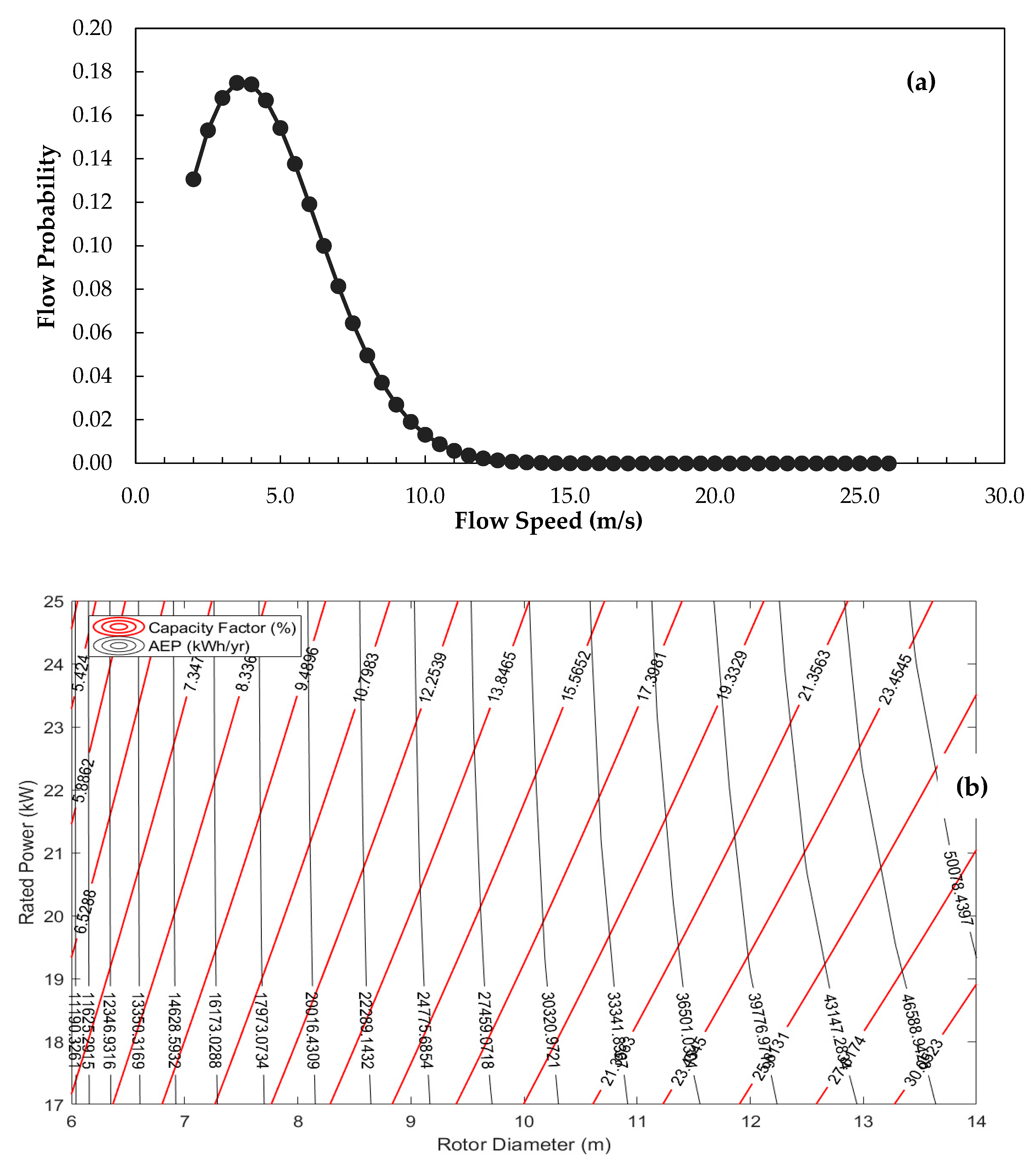
3.1. Wind Data Modelling

Australia has significant wind resources, and many of the best places are located in New South Wales. Wind speed plays a vital role in the performance of the wind turbine, since it is the primary source of energy. Wind speeds at a specific site vary according to annual, seasonal, and daily changes. It is crucial to conduct a statistical analysis with a probability distribution to study the potential of wind resources. Deniliquin is located in the Riverina region of New South Wales close to the border with Victoria, Australia. This area functions economically as a service center for the surrounding agricultural area. Thus, in this area, small wind turbines could be used for a remote, small electrical generation and agricultural application project. The wind data of the Deniliquin Airport AWS station (station number 074258) were chosen to analyze the wind energy potentials in this study. This station has a coordinate of −35.56, 144.95, and an elevation of 94.0 m. It is necessary to use some statistical analysis for the wind data. The probability distribution describes the occurrence frequency of wind speed [32]. Observations for the period from June 2018 to July 2019 were studied using Weibull probability density function. The Weibull probability density function, as shown in Equation 2, depends on two factors: scale and shape factor [33,34].

$$f\left(v\right)=\frac{k}{c} {\left(\frac{v}{c}\right)}^{k-1}\exp \left[-{\left(\frac{v}{c}\right)}^k\right]$$

(3)

where, k is the shape factor (dimensionless), c is the scale factor (m/s), and v is the wind speed (m/s) [35]. The shape parameter decides the curvature of the probability distribution; any variation in the shape parameter is affected by the estimated wind potential. Determination of the Weibull probability density function requires defining the shape and scale parameters, using different estimation methods. Employing the maximum likelihood method is typically done for defining shape and scale parameters as seen in the following equations [36,37]:

$$k={\left(\frac{{\sum }_{i=1}^n{v}_i{}^k\ln \left(v_i\right)}{{\sum }_{i=1}^n v_i{}^k}-\frac{{\sum }_{i=1}^n\ln \left(v_i\right)}{n}\right)}^{-1}$$

(4)

$$c={\left(\frac{{\sum }_{i=1}^n{v}_i{}^k}{n}\right)}^{\frac{1}{k}}$$

(5)

where v_i is the wind speed at (i) time, and n is the number of readings of wind speed data [38,39]. To define the AEP of the wind turbine, the probability distribution f (v) is combined with the power curve of wind turbine P (v) as shown in the following equation:

$$\mathrm{AEP}={{\displaystyle \int }}_{v_{cut,in}}^{v_{cut,out}}P\left(v\right) f\left(v\right)dv$$

(6)

where $v_{cut,in}$ is the cut-in wind speed (m/s), and $v_{cut,out}$ is the cut-out wind speed (m/s).

Assessment of the available resource at Deniliquin was defined by the shape and scale of the Weibull probability density function. The shape and scale factors are used as inputs for the optimization process, of which the objective is to maximize the AEP of a 20 kW wind turbine depending on the wind speed data in Deniliquin. The following section describes the optimization methodology.

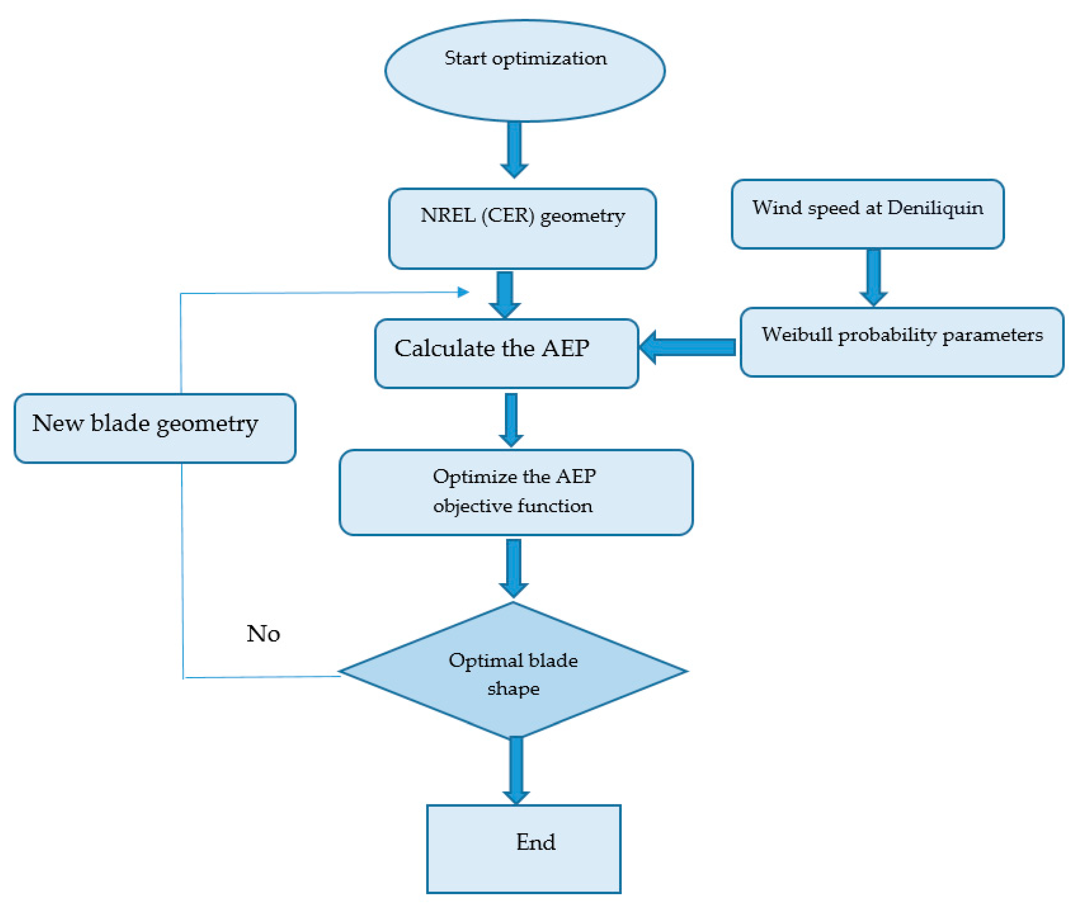
3.2. Optimization Blade Shape Methodology

National Renewable Energy Labs (NREL) developed HARP_Opt in the USA [40]. The HARP_Opt open-source code is used to conduct the horizontal axis rotor performance optimization process. The HARP_Opt gathers a BEM theory code with a genetic algorithm (GA) code to optimize and design the wind turbine’s rotor shape. Genetic algorithms [41] are evolutionary algorithms, and they are robust and reliable search techniques depending on the mechanism of natural selection [42]. The optimization process of the GA is done by iterating a set of individual solutions, where a set of solutions is called a population. An iteration is carried out from one population to the next to obtain subsequent populations of superior individuals. The WT_Perf software (National Renewable Energy Laboratory, Golden, CO, USA) [43] is used as the essential BEM code in HARP_Opt. The WT_Perf is developed to analyze the aerodynamic performance of the wind turbine using the BEM code. The HARP_Opt uses the WT_Perf code to predict the performance of the rotor wind turbine and the MATLAB GA code to carry out the optimization. The HARP_Opt could be used for a single or multiple objective optimization code for the objective function in the HARP_Opt software, either maximization of the AEP of the wind turbine or wind turbine efficiency.

3.2.1. Design Variables and Objective Function

The blade shape of the wind turbine is defined by the airfoil, chord length, and twist angle of each section along the blade. The validated wind turbine model of 20 kW, which has been discussed before, is used as a baseline for the optimization process and the same family of S809 airfoil was used. The airfoil lift and drag polar was done using spreadsheet AirfoilPrep v2.02 (v2.02.03, Windward Engineering, LLC, USA) This type of Excel formatting was used to generate airfoil data to be imported into WT_Perf. After preparing the airfoil data file, the file was imported into HARP_Opt.

The objective of the optimization process was to maximize the AEP of 20 kW wind turbine depending on the wind speed data in Deniliquin using the output of optimal chord length and twist distributions along the wind turbine blade. In this study, a single objective method was considered where the optimization was focused on the optimization of the aerodynamic shape without including structural optimization studies [44,45,46,47,48]. The Bezier curves were used to define the chord length and twist angle distributions to smooth the span-wise distribution along the blade. There were five control points for each chord length and twist angle parameters; thus, the total overall decision variables amounted to 25 control points. The same rated power, the rotor diameter, and the hub height were used as input in HARP_Opt, with the baseline validated wind turbine model as shown in Figure 5. In this study, the variable rotor speed and variable pitch control were used for the control system to produce more energy output [32]. The allowable rotor speeds range from 25 rpm to 150 rpm.

Table 3. Turbine configurations.

Wind Turbine Parameters	Value
Rotor diameter	11 m
Rated power capacity	20 kW
Number of blade segment	30 m
Number of blades	3
Hub diameter	0.6
Hub distance from the bottom surface	13 m
Air density	1.225 kg/s

below summarizes different parameters of turbine configurations.

3.2.2. Constraints

Specific design parameters should be in place to generate acceptable blade geometry [28,49,50] which are described in Appendix A. As shown in

Table 4. Genetic algorithm (GA) configuration.

Radial Position	1.25	1.535	2.345	3.565	5.5
Twist angle (degree)
Minimum	−10	−10	−10	−10	−10
Maximum	25	17	5	3	−1
Chord Length (m)
Minimum	0.5	0.1	0.1	0.1	0.1
Maximum	0.8	0.72	0.65	0.55	0.37

, the lower and upper bounds represent the five control sections’ control twist and chord values, respectively.

Trial and error were used to tune the GA’s parameters. The values input into this optimization run were the final ones after using trial and error.

Table 5. Genetic algorithm configuration.

Optimization Parameters	Value
Population size	200
Generation	150
The cross-over fraction	0.25
Error tolerance for the GA fitness values	1 × 10−6

summarizes the GA configuration employed.

4. Results and Discussion

4.1. Model Validation

This section firstly investigates the effect of those four turbulence models on predicting the aerodynamic characteristics of the twisted wind turbine, where the mechanical torque and blade pressure distribution were used for model validation when compared with the NREL test results. Secondly, the differences among the turbulence models under different wind speeds that included stall conditions were captured by simulating the wind turbine. Thirdly, the main aerodynamic parameters, such as lift coefficient, were extracted at a different span-wise sections along the blade. Fourthly, and finally, the aerodynamic flow of the S809 airfoil was visualized under different angles of attack, and they revealed the variation of the flow from the attached separated flow conditions.

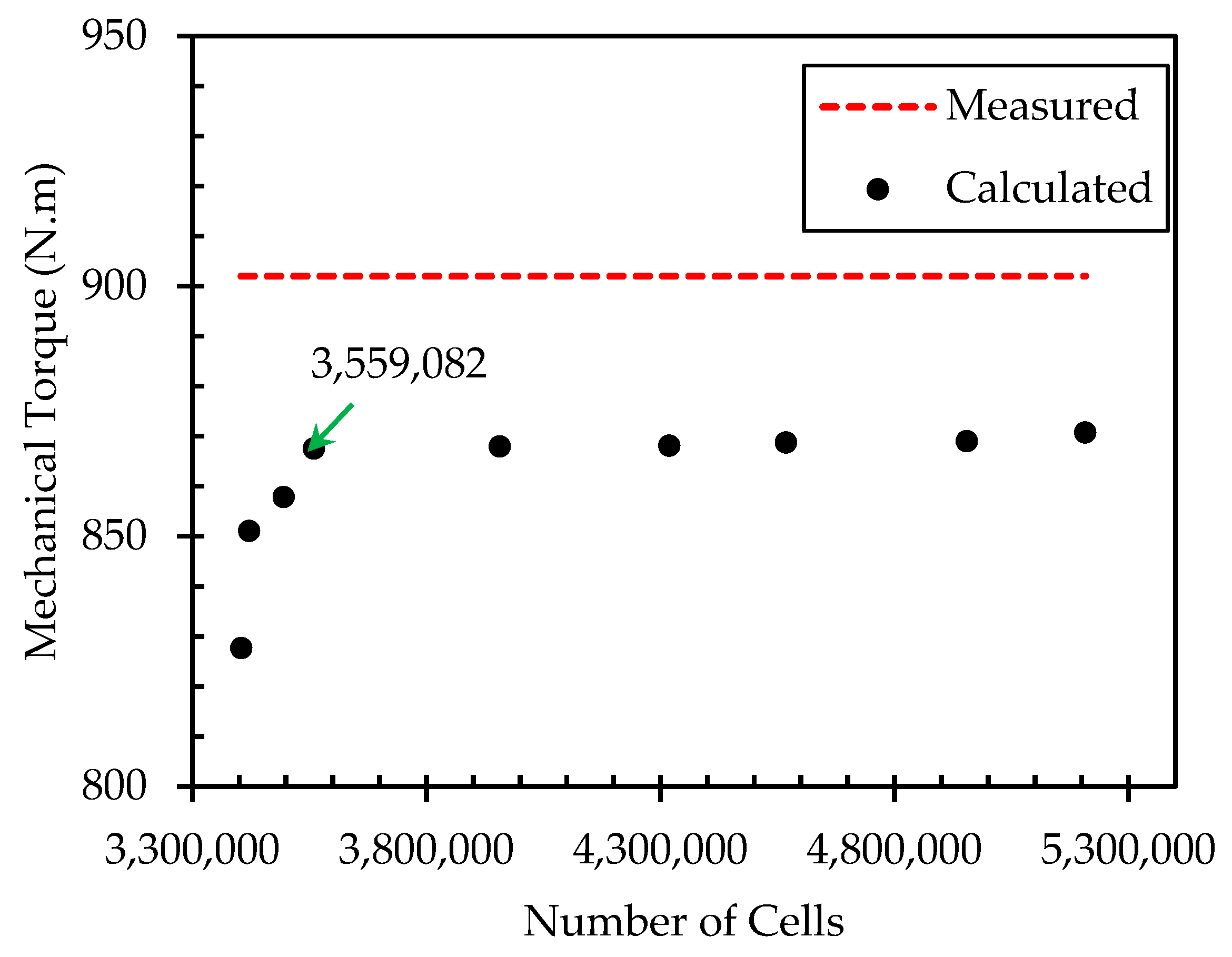
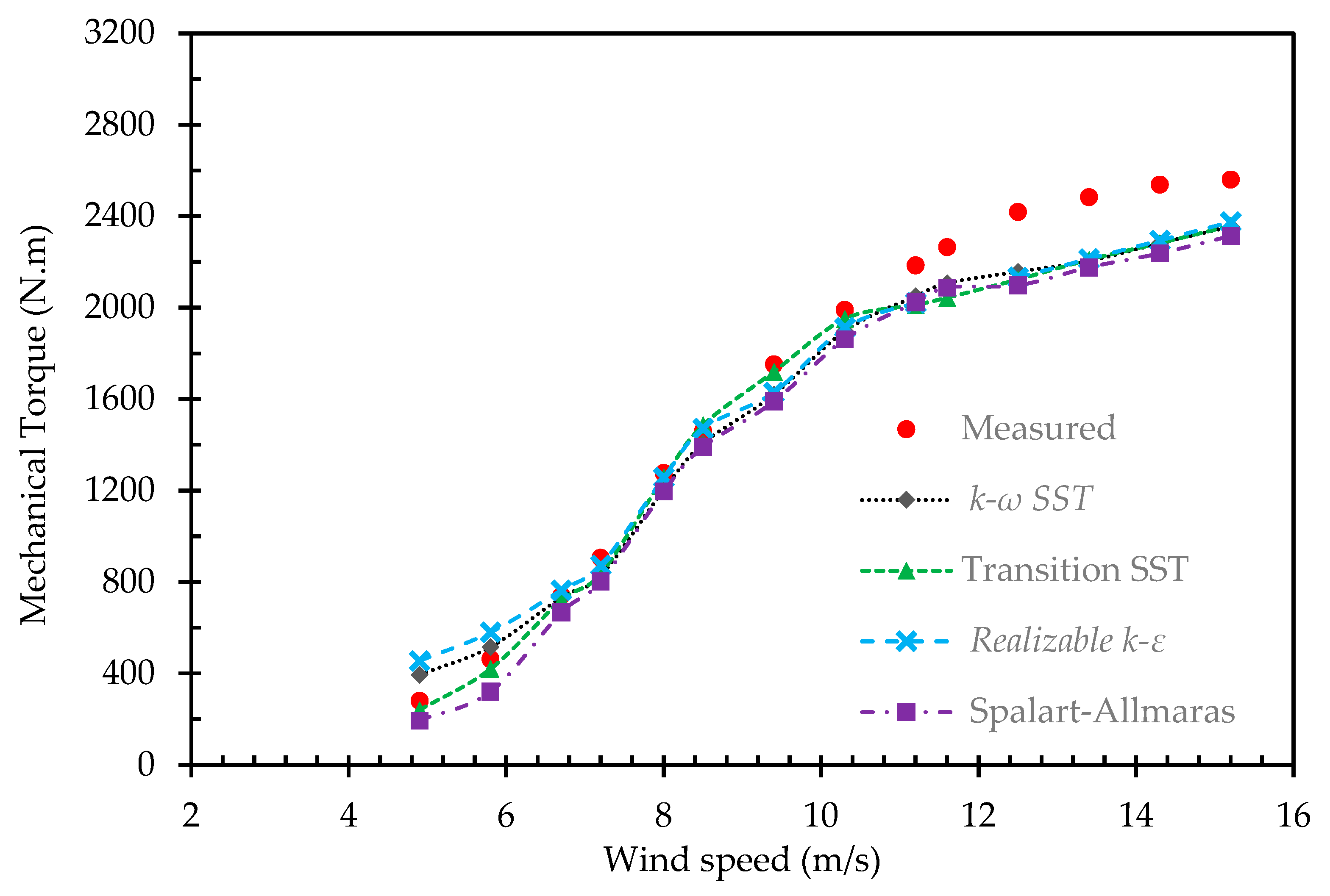
4.1.1. Mechanical Torque

Figure 6 compares the modelled shaft torque values using different RANS models and the measured results for the NREL rotor, which operated at a fixed speed of 72 rpm and a pitch angle of 5°. The CFD results demonstrated good agreement with the measurements at low and medium wind speeds between 4.9 and 9.0 m/s. Transition played an insignificant role in the prediction of the flow behavior of the wind turbine at this speed range. All RANS models made an excellent prediction of the flow around the wind turbine at the area where the flow was still attached.

It is important to note here that at a flow velocity between 9.0 and 10.5 m/s, the boundary layer was driven from the laminar to the turbulent transition area where the onset of a stall occurs. The transition SST model made the best prediction for that region due to the fact of its ability to resolve the laminar transition that considers the turbulent boundary layer which starts at the stall phenomenon. After 10 m/s, the results showed a marked difference for mechanical torque between the measured and RANS models. The significant separation of the flow and stall phenomena played a role in the difficulty of mechanical torque prediction using the RANS models.

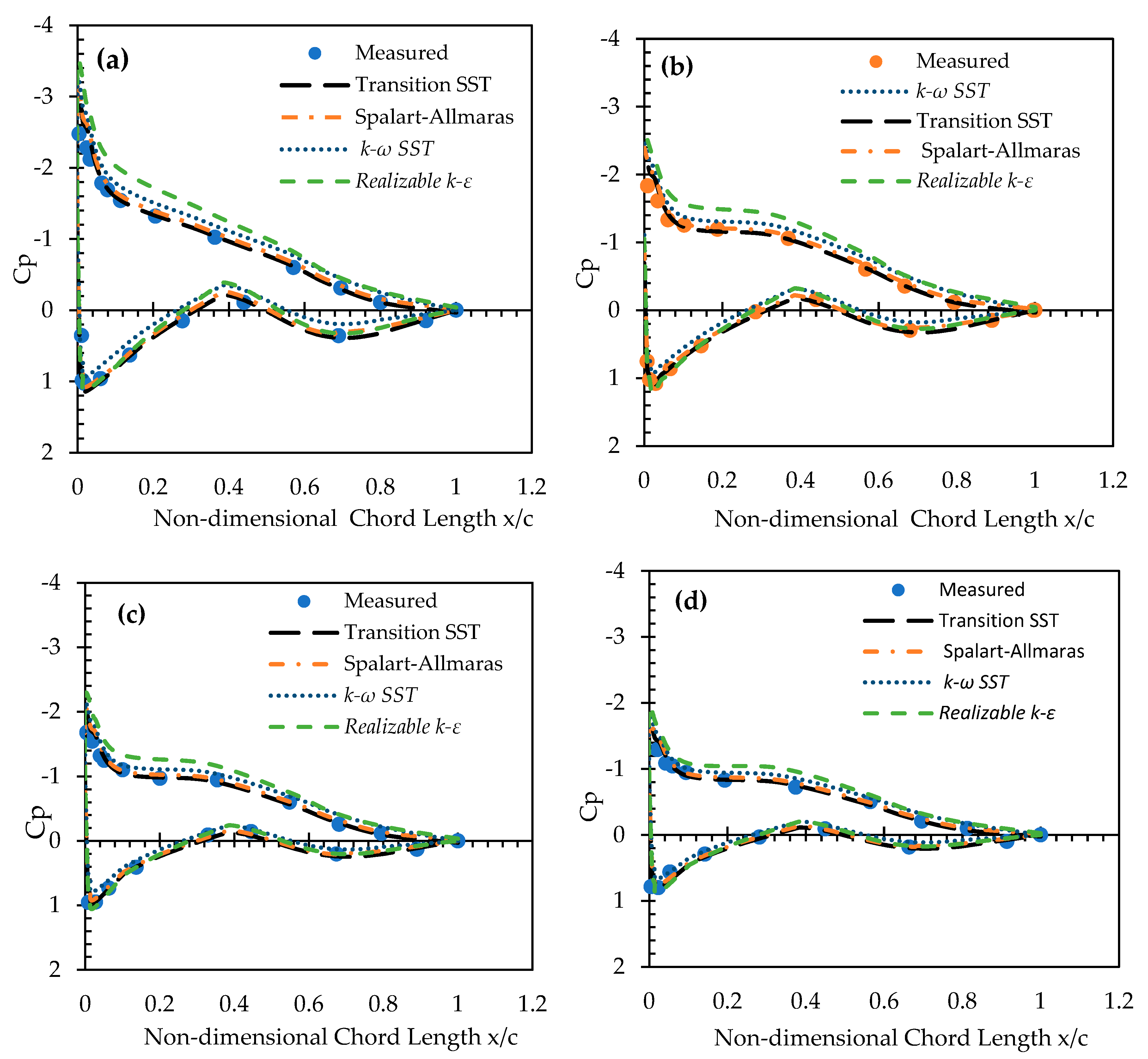
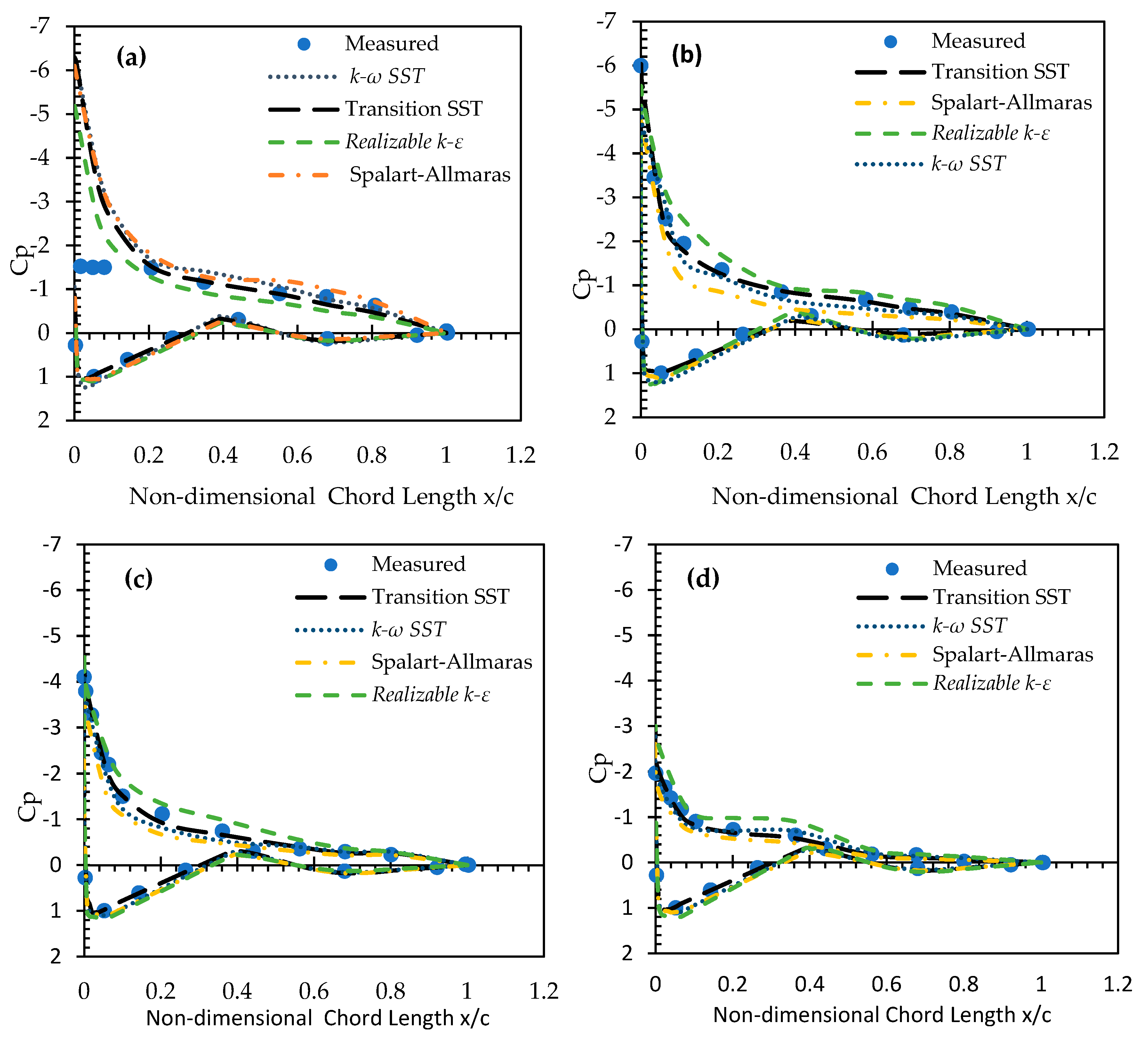
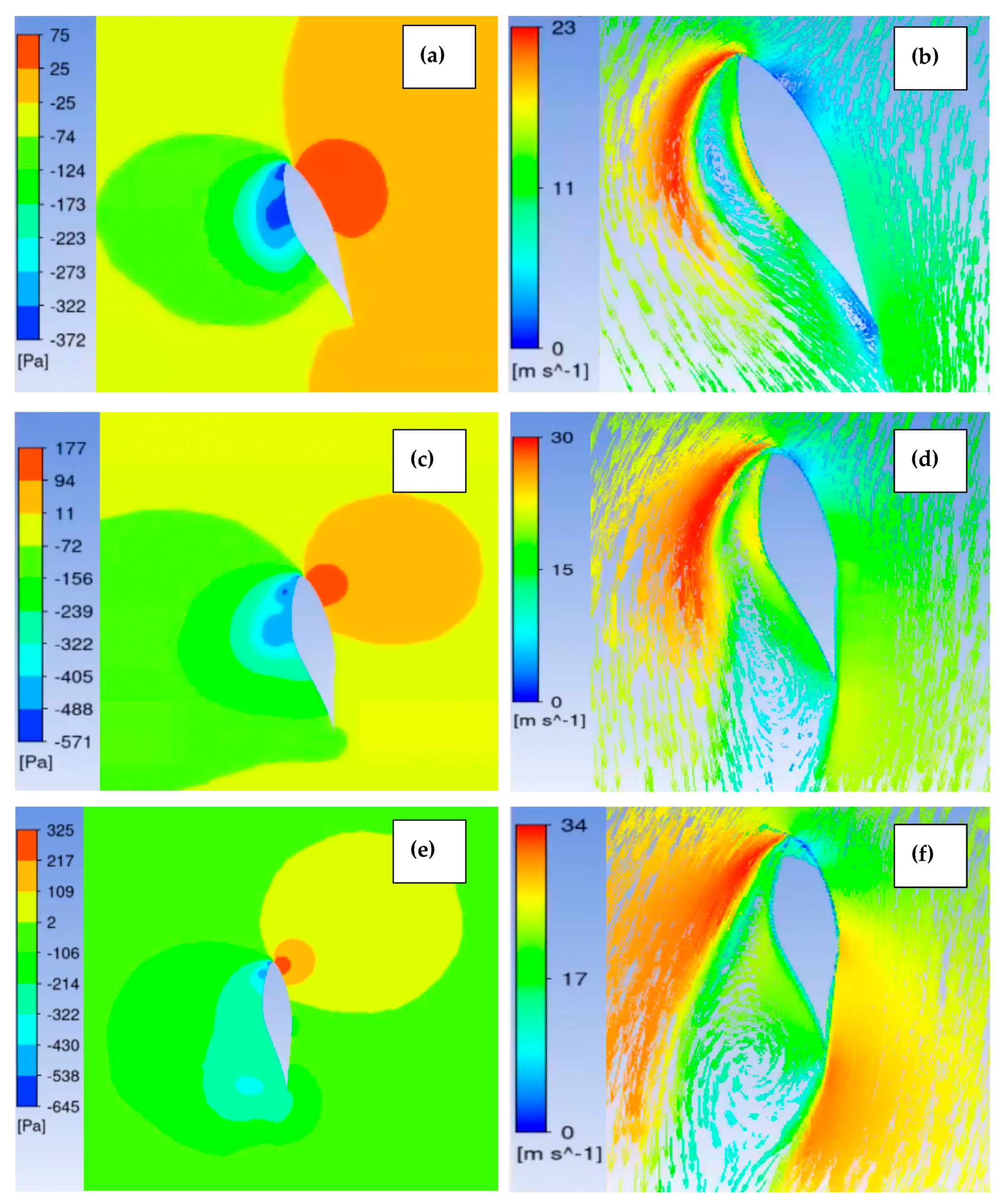
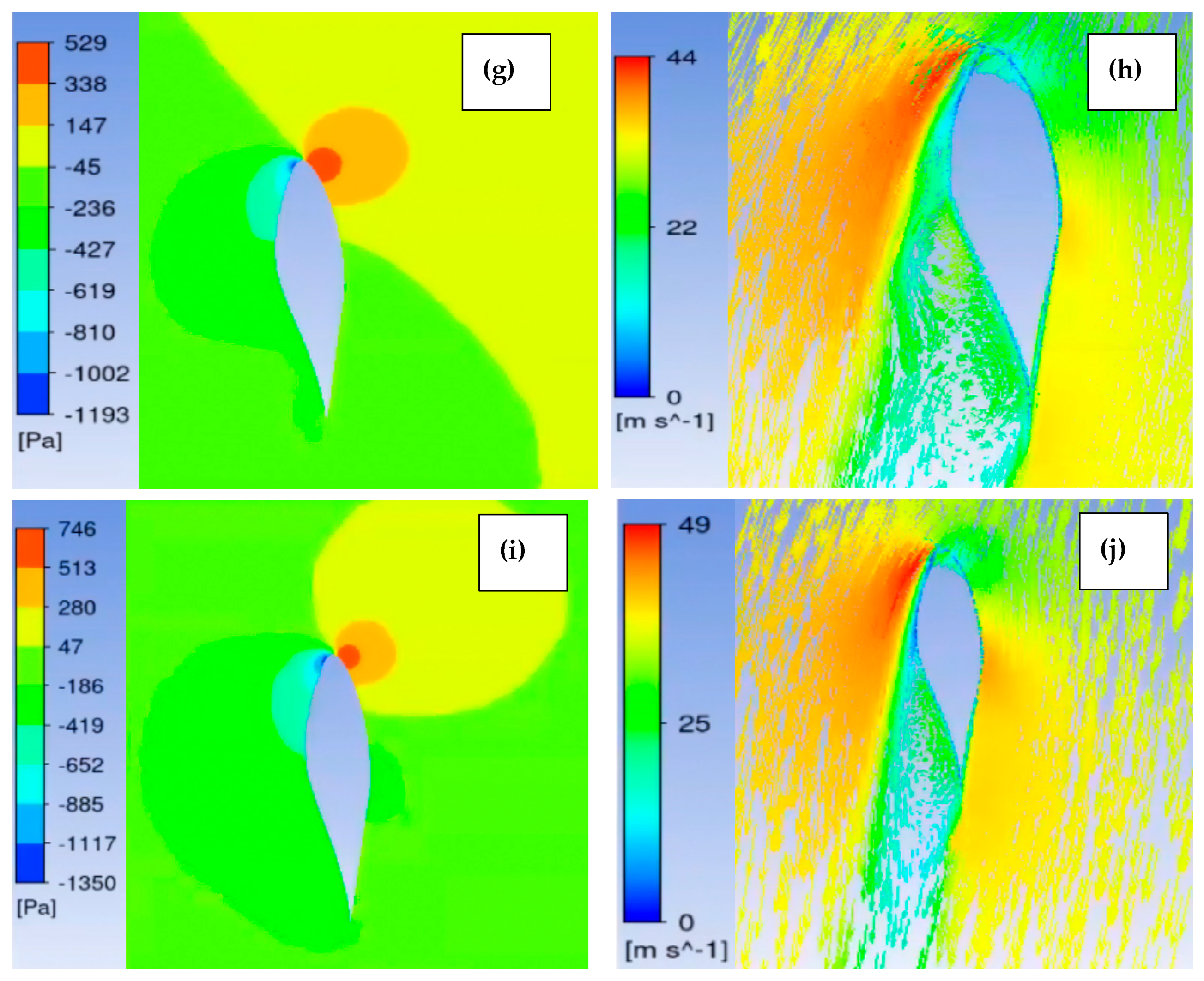
4.1.2. Pressure Distribution

Figure 7 and Figure 8 show comparisons of the measured and computed pressure coefficients at the four most important radial span sections (0.47 R, 0.63 R, 0.8 R, and 0.95 R) for two different wind speeds of 7.2 and 10.2 m/s. The pressure coefficient is calculated as in Equation (7):

$$Cp=\frac{P-P_{rel}}{0.5\rho \left(V_{rel}{}^2+{\left(r\Omega \right)}^2\right)}$$

(7)

where $P$ is the local static pressure, $P_{rel}$ is the free stream pressure, $V_{rel}$ is relative wind speed, Ω is the rotational wind speed (rad/s), $r$ is the radius of the section (m), and $\rho$ is the air density (kg/m³).

For a 7.2 m/s inlet wind speed, as shown in Figure 7, the modelled pressure distributions matched well with the experimental values, where the flow was almost attached to this wind speed with no stall boundary layer separation having yet started. Thus, all RANS models agreed well with the experimental data except realizable k-ε. In effect, this model had some limitations when the domain included two fluid zones, i.e., stationary and rotating zones [51]. In this case, non-physical turbulent viscosities were produced, and these affected the value of the turbulent viscosity. Since the present simulation had two domains, the realizable k-ε was not appropriate for predicting the current wind turbine simulation.

For an inlet wind speed of 10.2 m/s, which was classified as the onset of stall and shown in Figure 8, the best way to predict the airfoil’s pressure coefficient was to use the transition SST model. Any changes in the adverse pressure gradients would be reflected directly on the laminar boundary layer, and hence the early separation for the laminar boundary layer will happen when compared to the turbulent boundary layer. The transition SST model could predict the boundary layer for the flow region that changed from the laminar flow region to the turbulent transition region. Changing between boundary layers enabled the transition SST model to better predict the aerodynamic flow of the wind turbine for a stall wind condition when compared with other RANS models as shown in Figure 8a. At the 47% span location, the stall phenomena begin, and the separation was evident among the RANS models for predicting the wind turbine’s aerodynamics.

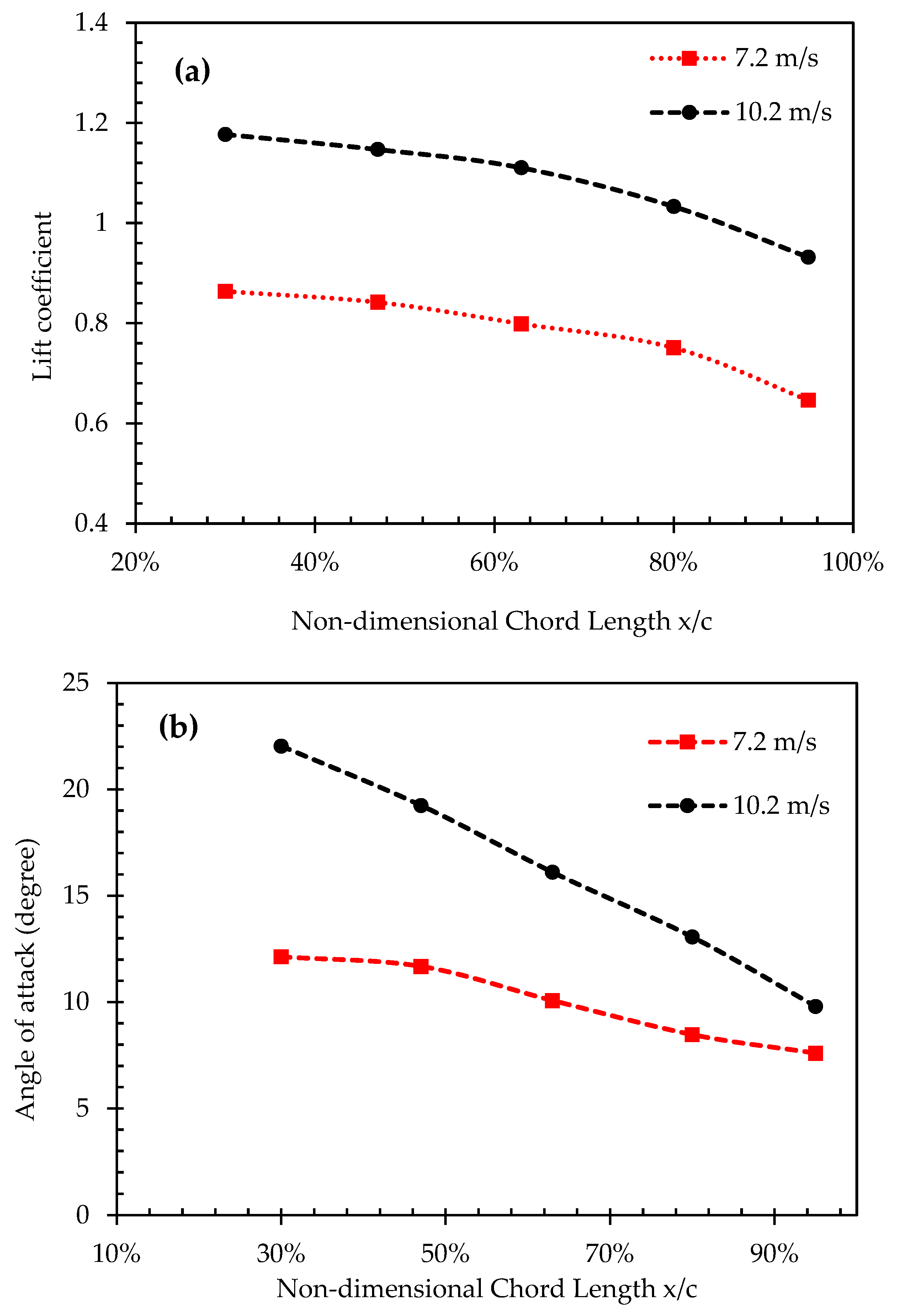
4.1.3. Investigation of the Airfoil Characteristics

It is essential to improve our understanding of the main aerodynamic characteristics of each section along the blade. Determination of the lift and drag coefficient of each airfoil section along the blade is a critical parameter for calculating the angle of attack. The Reynolds number increases as the wind speed rises, which affects the angle of attack and corresponding lift coefficient [52]. The results of the lift coefficient were obtained from simulation over NREL at a pitch angle equal to 5° and wind speeds varied from 4.9 to 15.2 m/s at a fixed angular speed, i.e., 72 rpm. As shown in Figure 9a, the lift coefficient varied with both radial sections and velocities.

As shown in Figure 9b, the calculated angle of attack had a high twist angle of 12.13° at 7.2 m/s wind speed on a plane through the blade at a distance of 1.51 m. At the same length, the angle of attack at 10.2 m/s was 22.04°. Thus, the angle of attack increased with increasing wind speed and decreased with the radial position. At 7.2 m/s near the hub region, minor transition and separation may occur due to the slightly high angle of attack, but the flow was still below the stall region and almost always attached. When increasing the wind velocity, the angle of attack increased at 10.2 m/s to the onset of stall. At this wind speed, the full separation occurred between the hub and 80% of the tip sections. Thus, the separation on the flow from the leading edge to the trailing edge occurred at 47% section of the blade and remained until 80% section.

The flow behavior at different airfoil sections along the blade was visualized around the airfoil with velocity and pressure contours. Transition SST indicated good results amongst the four turbulence models with the measurements shown above. As such, the velocity vectors and pressure contours results were predicted by the transition SST model. The blade cross-section at a 1.51 m radius investigated the flow on the inner region of the blade. In contrast, the blade cross-section at a 4.78 m radius studied the flow on the outer area of the blade. The figures below explain that the pressure fell to a small value as the flow over the airfoil accelerated. As the results in Figure 10a,c,e,g,i illustrate, the pressure coefficient dropped quickly to zero and reached a negative value. As the flow slowed down, the pressure increased, and the magnitude of the pressure coefficient decreased. As a result, the pressure of the lower surface became far more significant than the pressure of the upper surface, causing the blade to rotate. These results confirmed that the values of the pressure coefficient were negative at high air velocity. The separation will start when the flow on the upper surface at the trailing edge of the airfoil decelerates and mixes with the airflow from the lower surface. The point of flow separation happens earlier at larger angles of attack, and as the intensity of the adverse pressure rises, the separation point shifts forward on the airfoil.

As seen in Figure 10b,d,f,h,j, the velocity vectors on the airfoil sections varied following the differences of velocity along the blade. The velocity vectors increased from the root to the tip where the highest velocity vector was achieved by the outer section of the blade which was affected by the boundary layer separation [53]. The axial velocity increased at a uniform pattern along the blade, explaining the effect of the centrifugal force on the rotating blade.

The NREL CER wind turbine will use the original blade geometry design. The numerical modelling of this wind turbine will serve to investigate the mechanical output at different rotational speeds and variable pitch angles. Transition SST is the RANS model that was selected for use when the output power of the original blade geometry was compared with the optimized blade design. Transition SST can predict well the mechanical torque and the pressure distribution of different sections along the blade.

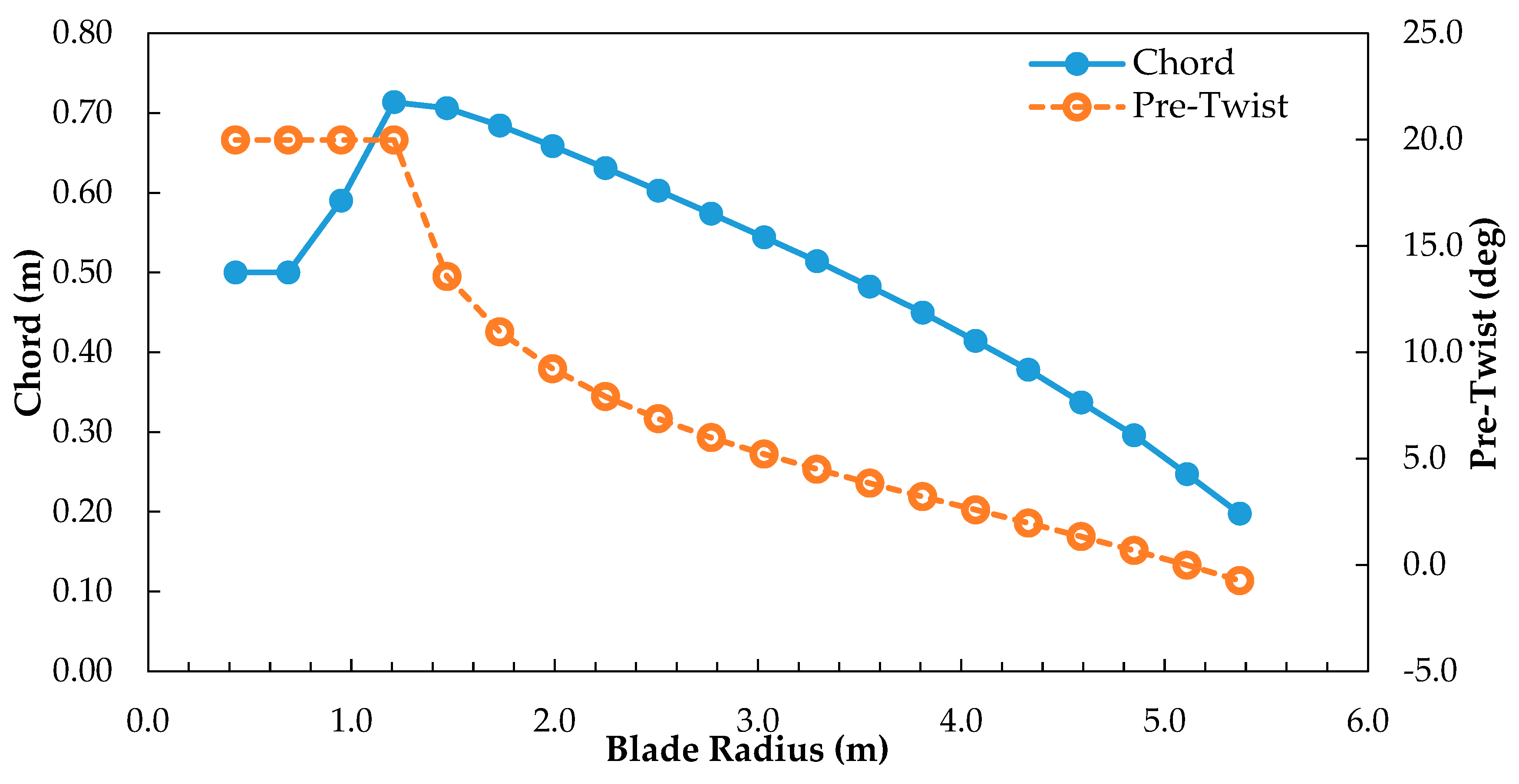
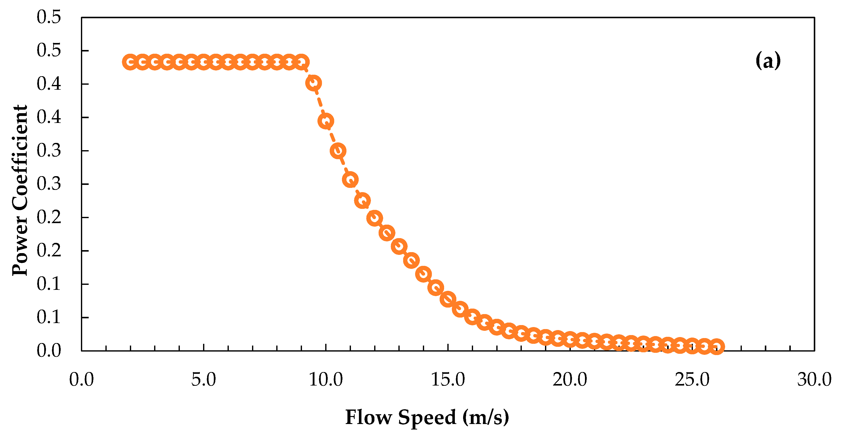
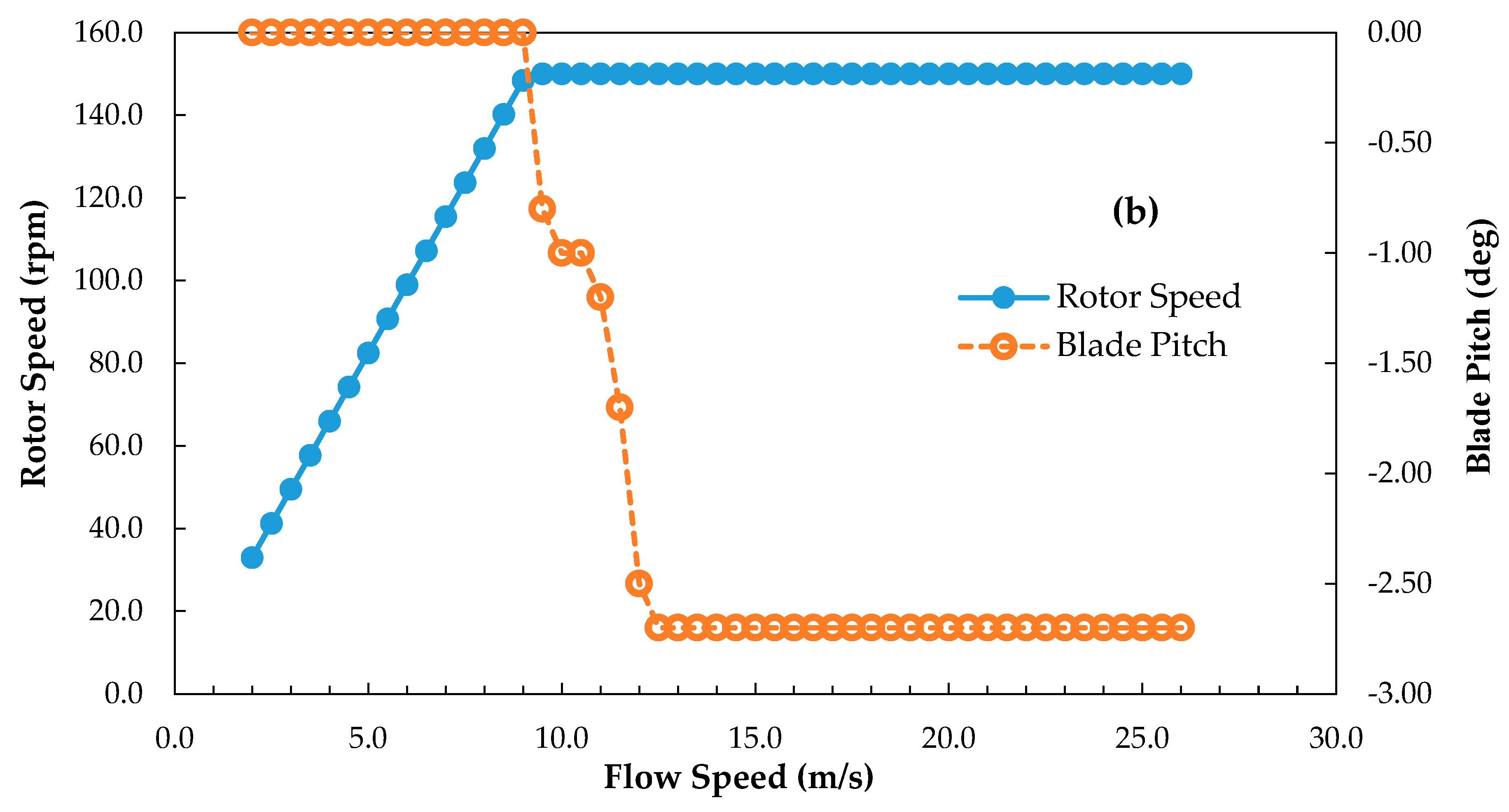
4.2. Optimization of Wind Turbine

The objective of this optimization process is to maximize the AEP at the Deniliquin site. It is essential to obtain the Weibull probability density function (see Figure 11a) to maximize the energy output. The Weibull function shape and scale parameters were defined as 2.096 and 5.042 m/s, respectively. The root mean square error (RMSE) and the coefficient of determination (R²) were used to evaluate the accuracy of the Weibull probability density function. The values of R² and RMSE were evaluated as 0.998587 and 0.013567, respectively. Those values reflected the fact that the Weibull probability distribution was very accurate in representing the recorded wind data. Depending on Weibull function parameters for the selected site and the 20kW rated capacity, the rotor diameter chosen seemed good with AEP as shown in Figure 11b.

In this study, the optimization process modified the shape of the blade design using chord and twist distribution along the blade. The chord and twist distributions of the optimized wind turbine blade are shown in Figure 12. The power coefficient of the optimized rotor with wind speed is depicted in Figure 13a.The power coefficient had the highest value of 0.433108 until the rated wind speed (9.5 m/s). Due to the Weibull probability density function being high in the low wind speed range, it is essential to have a high-power coefficient to increase the AEP. The blade pitch control is the variable pitch to stall angle; the control system will be able to brake the turbine at high winds safely. As shown in Figure 13b, the variation of rotor speed and pitch angle with different wind speeds shows the change of rotor speed and pitch angle with varying speeds of wind. The rotor speed at the cut-in speed (2 m/s) was approximately 32.98848 rpm. The pitch remained at 0°, while the rising wind speed improved the rotor speed to 148.4482 rpm at the rated speed of 9.5 m/s. The active pitch control began at this point and regulated the rotor speed to 150 rpm until 25 m/s was reached.

As seen below in Figure 14, the optimized rotor had a higher power output when compared to the reference rotor. According to Weibull probability density function for the Deniliquin site, 2 m/s speed was a well-suited value for cut-in speed. For the optimized rotor, a cut in the was is producing only 0.201682 kW which was approximately 1% of rated power capacity. As the wind speed rose to 8 m/s, the turbine output was 18.37828 kW with a power coefficient of 0.433108. This output was approximately 76% of the turbine’s rated capacity. At 9.5 m/s, the 20 kW rated power was reached. These differences between the power output of the tested and optimized rotor will be reflected in the AEP for the tested and optimized wind turbine. In this study, the AEP increased from 30,819.3 kW-hr/year in the original turbine to 33,614 kW-hr/year in the optimized wind turbine. Optimization improved the AEP by 9.068% when compared to the initial tested wind turbine design.

5. Conclusions

This study aimed to optimize the NREL (CER) wind turbine by CFD modelling. It investigated the aerodynamic characteristics of a 20 kW wind turbine at three-bladed twisted angles and tapered blades. Grid independence was achieved in terms of mechanical torque. As well, the study investigated the effect of four turbulence models in predicting the mechanical torque and pressure distributions. Simulated wind conditions varied from attached to separated flow conditions. Finally, a HARP_Opt code was used to optimize the wind turbine design using a genetic algorithm, aiming to maximize the AEP at the Deniliquin site. The major findings of this study are summarized as follows:

(1)

All four RANS models agreed well with experimental data at low wind speed ranges. Differences appeared among the four turbulence models as the wind speed increased;

(2)

At the onset of a stall condition of 10.2 m/s, the ttransition SST reported the best accuracy for predicting the pressure coefficient of the airfoil. The angle of attack increased with increasing wind speed and decreased with the radial position. The full separation occurred between the hub and 80% of the tip sections;

(3)

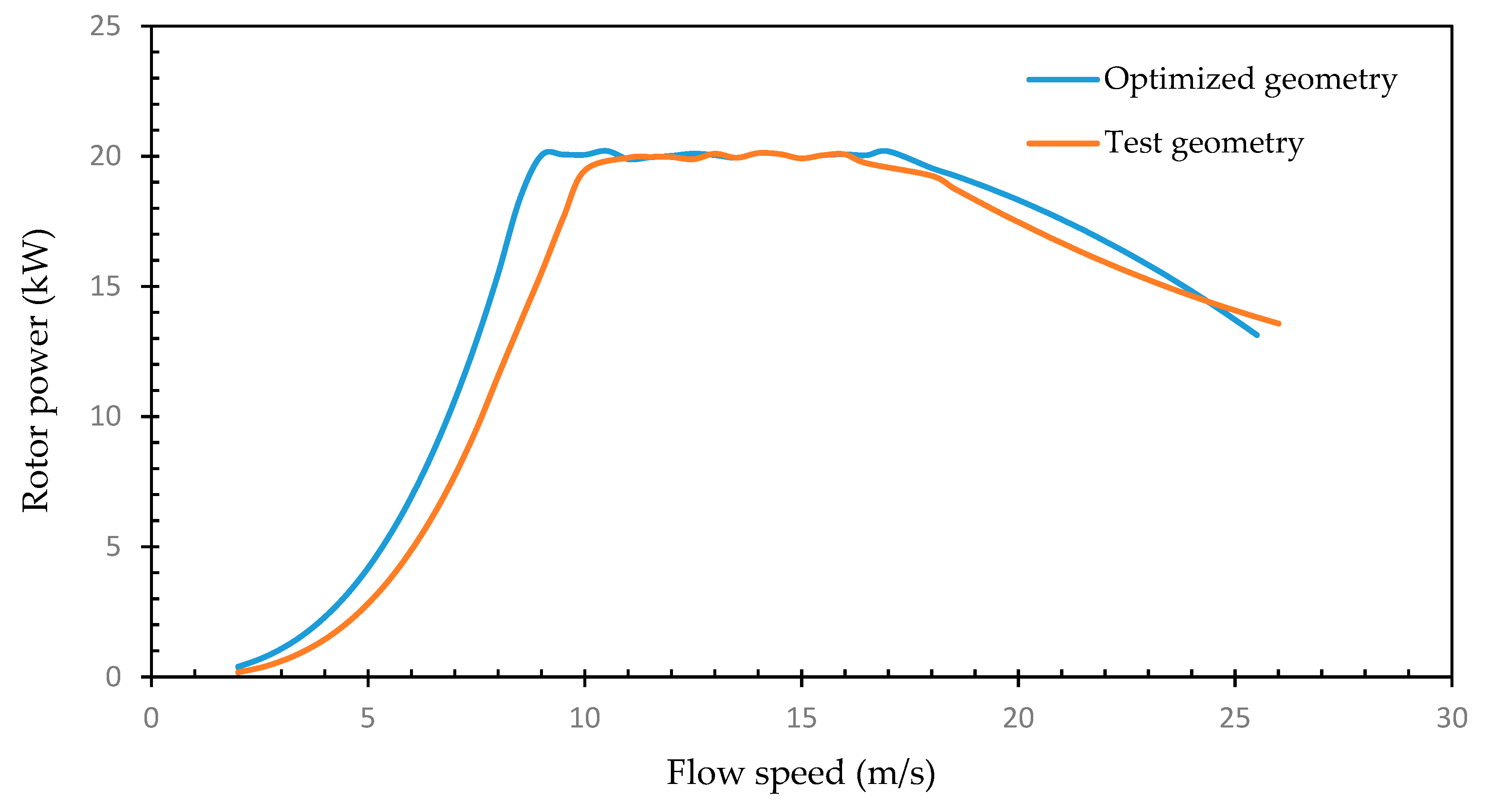
The shape of the rotor was modified by changing the chord and twist distribution along the blade, leading to 9.1% improvement in AEP.

References

1. Conti, J.; Holtberg, P.; Diefenderfer, J.; LaRose, A.; Turnure, J.T.; Westfall, L. International Energy Outlook 2016 with Projections to 2040; USDOE Energy Information Administration (EIA): Washington, DC, USA, 2016.
2. Sims, R.E.; Rogner, H.-H.; Gregory, K. Carbon emission and mitigation cost comparisons between fossil fuel, nuclear and renewable energy resources for electricity generation. Energy policy 2003, 31, 1315–1326. [Google Scholar] [CrossRef]
3. Wind Power Capacity Reaches 546 GW, 60 GW added in 2017; World Wind Energy Association: Bonn, Germany, 2018.
4. Kaviani, H.; Nejat, A. Aerodynamic noise prediction of a MW-class HAWT using shear wind profile. J. Wind Eng. Ind. Aerodyn. 2017, 168, 164–176. [Google Scholar] [CrossRef]
5. Ashrafi, Z.N.; Ghaderi, M.; Sedaghat, A. Parametric study on off-design aerodynamic performance of a horizontal axis wind turbine blade and proposed pitch control. Energy Convers. Manag. 2015, 93, 349–356. [Google Scholar] [CrossRef]
6. Alpman, E. Effect of selection of design parameters on the optimization of a horizontal axis wind turbine via genetic algorithm. In Proceedings of the Journal of Physics: Conference Series, Denpasar, Indonesia, 23–24 August 2016; p. 012044. [Google Scholar]
7. Darwish, A.S.; Shaaban, S.; Marsillac, E.; Mahmood, N.M. A methodology for improving wind energy production in low wind speed regions, with a case study application in Iraq. Comput. Ind. Eng. 2019, 127, 89–102. [Google Scholar] [CrossRef]
8. Liu, X.; Wang, L.; Tang, X. Optimized linearization of chord and twist angle profiles for fixed-pitch fixed-speed wind turbine blades. Renew. Energy 2013, 57, 111–119. [Google Scholar] [CrossRef]
9. Sedaghat, A.; Mirhosseini, M. Aerodynamic design of a 300 kW horizontal axis wind turbine for province of Semnan. Energy Convers. Manag. 2012, 63, 87–94. [Google Scholar] [CrossRef]
10. Plaza, B.; Bardera, R.; Visiedo, S. Comparison of BEM and CFD results for MEXICO rotor aerodynamics. J. Wind Eng. Ind.l Aerodyn. 2015, 145, 115–122. [Google Scholar] [CrossRef]
11. Li, Y.; Paik, K.-J.; Xing, T.; Carrica, P.M. Dynamic overset CFD simulations of wind turbine aerodynamics. Renew. Energy 2012, 37, 285–298. [Google Scholar] [CrossRef]
12. Lanzafame, R.; Mauro, S.; Messina, M. Wind turbine CFD modeling using a correlation-based transitional model. Renew. Energy 2013, 52, 31–39. [Google Scholar] [CrossRef]
13. Rajvanshi, D.; Baig, R.; Pandya, R.; Nikam, K. Wind turbine blade aerodynamics and performance analysis using numerical simulations. In Proceedings of the 11th Asian International Conference on Fluid Machinery, Chennai, India, 21–23 November 2011. [Google Scholar]
14. Moshfeghi, M.; Song, Y.J.; Xie, Y.H. Effects of near-wall grid spacing on SST-K-ω model using NREL Phase VI horizontal axis wind turbine. J. Wind Eng. Ind. Aerodyn. 2012, 107–108, 94–105. [Google Scholar] [CrossRef]
15. El Kasmi, A.; Masson, C. An extended k–ε model for turbulent flow through horizontal-axis wind turbines. J. Wind Eng. Ind. Aerodyn. 2008, 96, 103–122. [Google Scholar] [CrossRef]
16. AbdelSalam, A.M.; Ramalingam, V. Wake prediction of horizontal-axis wind turbine using full-rotor modeling. J. Wind Eng. Ind. Aerodyn. 2014, 124, 7–19. [Google Scholar] [CrossRef]
17. Abdelsalam, A.M.; Boopathi, K.; Gomathinayagam, S.; Kumar, S.H.K.; Ramalingam, V. Experimental and numerical studies on the wake behavior of a horizontal axis wind turbine. J. Wind Eng. Ind. Aerodyn. 2014, 128, 54–65. [Google Scholar] [CrossRef]
18. Siddiqui, M.S.; Rasheed, A.; Tabib, M.; Kvamsdal, T. Numerical analysis of NREL 5MW wind turbine: A study towards a better understanding of wake characteristic and torque generation mechanism. In Proceedings of the Journal of Physics: Conference Series, Denpasar, Indonesia, 23–24 August 2016; p. 032059. [Google Scholar]
19. Rütten, M.; Penneçot, J.; Wagner, C. Unsteady Numerical Simulation of the Turbulent Flow around a Wind Turbine. In Progress in Turbulence III; Springer: Berlin, Germany, 2009; pp. 103–106. [Google Scholar]
20. ANSYS. ANSYS Fluent Tutorial Guide, Release 18.0; ANSYS, Inc.: Pittsburgh, PA, USA, 2017. [Google Scholar]
21. Argyropoulos, C.; Markatos, N. Recent advances on the numerical modelling of turbulent flows. Appl. Math. Model. 2015, 39, 693–732. [Google Scholar] [CrossRef]
22. Rocha, P.A.C.; Rocha, H.H.B.; Carneiro, F.O.M.; Vieira da Silva, M.E.; Bueno, A.V. k–ω SST (shear stress transport) turbulence model calibration: A case study on a small scale horizontal axis wind turbine. Energy 2014, 65, 412–418. [Google Scholar] [CrossRef]
23. Spalart, P.; Allmaras, S. A one-equation turbulence model for aerodynamic flows. In Proceedings of the 30th Aerospace Sciences Meeting and Exhibit, Reno, NV, USA, 6–9 January 1992; p. 439. [Google Scholar]
24. Wang, S.; Ingham, D.B.; Ma, L.; Pourkashanian, M.; Tao, Z. Turbulence modeling of deep dynamic stall at relatively low Reynolds number. J. Fluids Struct. 2012, 33, 191–209. [Google Scholar] [CrossRef]
25. Hand, M.; Simms, D.; Fingersh, L.; Jager, D.; Cotrell, J.; Schreck, S.; Larwood, S. Unsteady Aerodynamics Experiment Phase VI: Wind Tunnel Test Configurations and Available Data Campaigns; National Renewable Energy Laboratory: Golden, CO, USA, 2001.
26. Giguere, P.; Selig, M. Design of a Tapered and Twisted Blade for the NREL Combined Experiment Rotor; National Renewable Energy Laboratory: Golden, CO, USA, 1999.
27. Akpinar, E.K.; Akpinar, S. A statistical analysis of wind speed data used in installation of wind energy conversion systems. Energy Convers. Manag. 2005, 46, 515–532. [Google Scholar] [CrossRef]
28. Lawson, M.J.; Li, Y.; Sale, D.C. Development and verification of a computational fluid dynamics model of a horizontal-axis tidal current turbine. In Proceedings of the 30th International Conference on Ocean, Offshore and Arctic Engineering (ASME 2011), Denver, CO, USA, 11–17 November 2011; pp. 711–720. [Google Scholar]
29. Somers, D.M. Design and Experimental Results for the S809 Airfoil; National Renewable Energy Laboratory: Golden, CO, USA, 1997.
30. Bouhelal, A.; Smaili, A.; Guerri, O.; Masson, C. Numerical investigation of turbulent flow around a recent horizontal axis wind Turbine using low and high Reynolds models. J. Appl. Fluid Mech. 2018, 11, 151–164. [Google Scholar] [CrossRef]
31. Bourdin, P.; Wilson, J.D. Windbreak aerodynamics: Is computational fluid dynamics reliable? Boundary-Layer Meteorol. 2008, 126, 181–208. [Google Scholar] [CrossRef]
32. Infield, D.; Freris, L. Renewable Energy in Power Systems; John Wiley & Sons: Hoboken, NJ, USA, 2020. [Google Scholar]
33. Manwell, J.F.; McGowan, J.G.; Rogers, A.L. Wind Energy Explained: Theory, Design and Application; John Wiley & Sons: Hoboken, NJ, USA, 2010. [Google Scholar]
34. Katsigiannis, Y.A.; Stavrakakis, G.S. Estimation of wind energy production in various sites in Australia for different wind turbine classes: A comparative technical and economic assessment. Renew. Energy 2014, 67, 230–236. [Google Scholar] [CrossRef]
35. Bai, C.-J.; Chen, P.-W.; Wang, W.-C. Aerodynamic design and analysis of a 10 kW horizontal-axis wind turbine for Tainan, Taiwan. Clean Technol. Environ. Policy 2016, 18, 1151–1166. [Google Scholar] [CrossRef]
36. Rocha, P.A.C.; de Sousa, R.C.; de Andrade, C.F.; da Silva, M.E.V. Comparison of seven numerical methods for determining Weibull parameters for wind energy generation in the northeast region of Brazil. Appl. Energy 2012, 89, 395–400. [Google Scholar] [CrossRef]
37. Seguro, J.; Lambert, T. Modern estimation of the parameters of the Weibull wind speed distribution for wind energy analysis. J. Wind Eng. Ind. Aerodyn. 2000, 85, 75–84. [Google Scholar] [CrossRef]
38. Lydia, M.; Kumar, S.S.; Selvakumar, A.I.; Kumar, G.E.P. A comprehensive review on wind turbine power curve modeling techniques. Renew. Sustain. Energy Rev. 2014, 30, 452–460. [Google Scholar] [CrossRef]
39. Yingcheng, X.; Nengling, T. Review of contribution to frequency control through variable speed wind turbine. Renew. Energy 2011, 36, 1671–1677. [Google Scholar] [CrossRef]
40. Sale, D.C. HARP_Opt User’s Guide. NWTC Design Codes. 2010. Available online: http://wind.nrel.gov/designcodes/simulators/HARP_Opt/Lastmodified (accessed on 11 March 2020).
41. Selig, M.S.; Coverstone-Carroll, V.L. Application of a genetic algorithm to wind turbine design. J. Energy Resour. Technol. 1996, 118, 22–28. [Google Scholar] [CrossRef] [Green Version]
42. Zhang, T.-T.; Wang, Z.-G.; Huang, W.; Yan, L. Parameterization and optimization of hypersonic-gliding vehicle configurations during conceptual design. Aerosp. Sci. Technol. 2016, 58, 225–234. [Google Scholar] [CrossRef]
43. Platt, A.; Buhl, M. Wt Perf User Guide for Version 3.05; National Renewable Energy Laboratory: Golden, CO, USA, 2012.
44. Kröger, G.; Siller, U.; Dabrowski, J. Aerodynamic Design and Optimization of a Small Scale Wind Turbine. In Proceedings of the ASME Turbo Expo 2014: Turbine Technical Conference and Exposition, Dusseldorf, Germany, 16–20 June 2014. [Google Scholar]
45. Ceyhan, O. Aerodynamic design and optimization of horizontal axis wind turbines by using BEM theory and genetic algorithm. Middle East Tech. Univ. 2008. Available online: http://etd.lib.metu.edu.tr/upload/12610024/index.pdf (accessed on 11 March 2020).
46. Wang, L.; Tang, X.; Liu, X. Optimized chord and twist angle distributions of wind turbine blade considering Reynolds number effects. Wind Energy 2012. Available online: https://www.researchgate.net/profile/Lin_Wang120/publication/258994126_Optimized_chord_and_twist_angle_distributions_of_wind_turbine_blade_considering_Reynolds_number_effects/links/54ccebc10cf24601c08c6f46.pdf (accessed on 11 March 2020).
47. Vučina, D.; Marinić-Kragić, I.; Milas, Z. Numerical models for robust shape optimization of wind turbine blades. Renew. Energy 2016, 87, 849–862. [Google Scholar] [CrossRef]
48. Shen, X.; Yang, H.; Chen, J.; Zhu, X.; Du, Z. Aerodynamic shape optimization of non-straight small wind turbine blades. Energy Convers. Manag. 2016, 119, 266–278. [Google Scholar] [CrossRef] [Green Version]
49. Hassanzadeh, A.; Hassanabad, A.H.; Dadvand, A. Aerodynamic shape optimization and analysis of small wind turbine blades employing the Viterna approach for post-stall region. Alex. Eng. J. 2016, 55, 2035–2043. [Google Scholar] [CrossRef] [Green Version]
50. Seo, J.; Yi, J.-H.; Park, J.-S.; Lee, K.-S. Review of tidal characteristics of Uldolmok Strait and optimal design of blade shape for horizontal axis tidal current turbines. Renew. Sustain. Energy Rev. 2019, 113, 109273. [Google Scholar] [CrossRef]
51. Hamada, K.; Smith, T.; Durrani, N.; Qin, N.; Howell, R. Unsteady flow simulation and dynamic stall around vertical axis wind turbine blades. In Proceedings of the 46th AIAA Aerospace Sciences Meeting and Exhibit, Reno, NV, USA, 7–10 January 2008; p. 1319. [Google Scholar]
52. Ge, M.; Tian, D.; Deng, Y. Reynolds number effect on the optimization of a wind turbine blade for maximum aerodynamic efficiency. J. Energy Eng. 2014, 142, 04014056. [Google Scholar] [CrossRef]
53. Du, Z.; Selig, M.S. The effect of rotation on the boundary layer of a wind turbine blade. Renew. Energy 2000, 20, 167–181. [Google Scholar] [CrossRef]
54. Launder, B.E.; Sharma, B. Application of the energy-dissipation model of turbulence to the calculation of flow near a spinning disc. Lett. Heat Mass Transf. 1974, 1, 131–137. [Google Scholar] [CrossRef]
55. Shih, T.-H.; Liou, W.W.; Shabbir, A.; Yang, Z.; Zhu, J. A new k-ϵ eddy viscosity model for high reynolds number turbulent flows. Comput. Fluids 1995, 24, 227–238. [Google Scholar] [CrossRef]
56. Yakhot, V.; Orszag, S.; Thangam, S.; Gatski, T.; Speziale, C. Development of turbulence models for shear flows by a double expansion technique. Phys. Fluids A Fluid Dyn. 1992, 4, 1510–1520. [Google Scholar] [CrossRef] [Green Version]
57. Tikhomirov, V. Equations of turbulent motion in an incompressible fluid. In Selected Works of AN Kolmogorov; Springer: Berlin, Germany, 1991; pp. 328–330. [Google Scholar]
58. Wilcox, D.C. Formulation of the kw turbulence model revisited. AIAA J. 2008, 46, 2823–2838. [Google Scholar] [CrossRef] [Green Version]
59. Menter, F.R. Review of the shear-stress transport turbulence model experience from an industrial perspective. Int. J. Comput. Fluid Dyn. 2009, 23, 305–316. [Google Scholar] [CrossRef]
60. Gatski, T.B.; Rumsey, C.L.; Manceau, R. Current trends in modelling research for turbulent aerodynamic flows. Philos. Trans. R. Soc. A Math. Phys. Eng. Sci. 2007, 365, 2389–2418. [Google Scholar] [CrossRef] [PubMed]
61. Spalart, P.; Shur, M. On the sensitization of turbulence models to rotation and curvature. Aerosp. Sci. Technol. 1997, 1, 297–302. [Google Scholar] [CrossRef]
62. Rahman, M.; Siikonen, T.; Agarwal, R. Improved low-Reynolds-number one-equation turbulence model. AIAA J. 2011, 49, 735–747. [Google Scholar] [CrossRef]
63. Langtry, R.B.; Menter, F.R. Correlation-based transition modeling for unstructured parallelized computational fluid dynamics codes. AIAA J. 2009, 47, 2894–2906. [Google Scholar] [CrossRef]
64. Calomino, F.; Alfonsi, G.; Gaudio, R.; D’Ippolito, A.; Lauria, A.; Tafarojnoruz, A.; Artese, S. Experimental and numerical study of free-surface flows in a corrugated pipe. Water 2018, 10, 638. [Google Scholar] [CrossRef] [Green Version]
65. Xudong, W.; Shen, W.Z.; Zhu, W.J.; Sørensen, J.N.; Jin, C. Shape optimization of wind turbine blades. Wind Energy 2009, 12, 781–803. [Google Scholar] [CrossRef]
66. Li, Y.; Yi, J.-H.; Sale, D. Recent improvement of optimization methods in a tidal current turbine optimal design tool. 2012 Oceans 2012, 1–8. [Google Scholar] [CrossRef]
Figure 1. (a) A 3D geometry model of a 20 kW wind turbine blade. (b) The chord and twist distribution along the span of the blade.
Energies 13 02292 g001
Figure 2. (a) Computational domain; (b) computational mesh generation, and (c) cell meshing around the rotor.
Energies 13 02292 g002aEnergies 13 02292 g002b
Figure 3. Grid sensitivity.
Energies 13 02292 g003
Figure 4. Numerical modelling of HAWT.
Energies 13 02292 g004
Figure 5. Optimization flowchart.
Energies 13 02292 g005
Figure 6. Mechanical torque.
Energies 13 02292 g006
Figure 7. Comparison of span-wise pressure distribution among the different turbulence models and NREL measurements at 7.2 m/s for: (a) 47% section, (b) 63% section, (c) 80% section, and (d) 95% section.
Energies 13 02292 g007
Figure 8. Comparison of span-wise pressure distribution among the different turbulence models and NREL measurements at 10.2 m/s for: (a) 47% section, (b) 63% section, (c) 80% section, and (d) 95% section.
Energies 13 02292 g008
Figure 9. (a) Variation of lift coefficient with different non-dimensional chord length sections along the blade. (b) Variation of the angle of attack with different non-dimensional chord length sections along the blade.
Energies 13 02292 g009
Figure 10. Pressure and velocity vector distributions at 7.2 m/s of different span stations: (a) pressure and (b) velocity vector of 30% span; (c) pressure and (d) velocity vector of 47% span; (e) pressure and (f) velocity vector of 63% span; (g) pressure and (h) velocity vector of 80% span; and (i) pressure and (j) velocity vector of 95% span.
Energies 13 02292 g010aEnergies 13 02292 g010b
Figure 11. (a) Weibull probability density function at the Deniliquin site. (b) The AEP for different turbine diameters for Weibull function parameters: k = 2.096 and c = 5.042 m/s.
Energies 13 02292 g011
Figure 12. Twist angle and Chord length distribution along the blade.
Energies 13 02292 g012
Figure 13. (a) Variation of power coefficient with wind speeds. (b) Change of rotor speed and pitch angle with wind speeds.
Energies 13 02292 g013aEnergies 13 02292 g013b
Figure 14. Power output of the reference tested rotor and optimized rotor.
Energies 13 02292 g014