1. Introduction
Globally, the installed wind power capacity has increased more than six-fold within eleven years, from 93.9 GW in 2007 to 591.5.8 GW in 2018. As of 2018, nearly one tenth of the global installed wind power capacity was located in Germany, where the installed wind power capacity increased from 22.2 GW in 2007 to 53.2 GW in 2018. This increase resulted in a power generation of 111.5 TWh in 2018, corresponding to 21% of the electricity demand in Germany [
1,
2,
3,
4].
Due to this significant expansion, the spatial and temporal availability of climate-dependent wind resources increasingly affects the whole power system. Consequently, assessments of the electricity system’s vulnerability to extreme climate events and climate change by means of power system models provide vital insights into how future electricity systems should be structured to mitigate supply scarcity and power outages [
5,
6,
7]. Therefore, accurate multi-year generation time series (i.e., multiple years of temporally highly-resolved values) are used as input data for power system models (e.g., [
8,
9]) as well as energy system models (e.g., [
10,
11,
12]), for quantifying the system’s resilience to climate events. This is increasingly important when an even higher market penetration of renewables is taken into account [
13].
In the recent past, mainly power curve-based models based on reanalysis climate data sets [
13,
14,
15,
16,
17,
18,
19] have been used for deriving multi-year time series. These models have been able to reproduce wind power generation time series sufficiently well in terms of error metrics, and distributional and seasonal characteristics. However, these models also feature possible drawbacks, such as the high data requirements for model setup (i.e., wind turbine locations, turbine specifications, and commissioning dates) and the need for separate work steps for bias correction and the replication of wake effects (e.g., power curve smoothing) [
13,
18,
19]. In particular, well known shortcomings of reanalysis data, i.e., a significant mean bias in wind speeds, have to be overcome by the models via bias correction [
19], which relies on the availability of historical wind power generation time series or independent sources of wind speed data, such as local wind speed measurements. Another downside of reanalysis-based time series generated by power curve-based models has been their insufficient replication of extreme generation events and short-term power ramps [
13,
15,
18]. This can only partly be attributed to the methodology, as the underlying reanalysis data sources do not sufficiently capture extreme situations [
18]. The accurate replication of power generation extremes and potential generation changes within short- (1 h), mid- (3 and 6 h), and long-term (12 h) timeframes, however, would be of high value for power system models.
As real-generation time series are necessary for bias-correction or validation anyhow, instead of using power curve-based models, machine learning (ML) models can be applied to derive synthetic time series from climate data for time periods where no observed generation is available.
In particular, neural networks are a promising approach. They can fit arbitrary, non-linear functions as they are universal function approximators [
20]. The need for a correction of systematic biases as a separate work step and the need for information on accurate turbine locations and other specifications can therefore possibly be overcome when using machine learning wind power generation models. This decreases the effort required when generating time series of wind power electricity generation, as gathering accurate information on turbine locations can be time-consuming or even impossible for some countries. Additionally, while machine learning (ML) models based on the same underlying climatic data cannot be expected to fully solve the problem of the correct representation of real wind power variability, they may increase the quality of results in terms of extreme values by learning spatio-temporal relationships between the climatic input and (extreme) values for the output.
In this paper, we consequently assessed whether machine learning (ML) models are equally or even better suited than Renewables.ninja (RN)—a cutting-edge power curve-based model time series [
13]—for replicating the distributional, seasonal, extreme value, and power ramp characteristics of actual wind power generation. Furthermore, we quantified how the quality of the ML modeled time series depends on the extent of information on wind turbine locations that the ML model receives. RN has been chosen as the comparison dataset because it is an openly available wind power dataset with a proven performance based on a state-of-the-art modeling approach. It has been found that RN wind power time series have more similarities to Transmission System Operator (TSO) data compared with EMHIRES [
18]—a second cutting-edge power curve-based time series. For a limited number of years (2012–2014), the RN wind power time series showed a correlation of 0.98 compared with TSO data [
21]. A multitude of research projects have successfully used the RN wind power dataset as a data source for assessing balancing of the wind power output via the spatial deployment of wind power, in order to understand the impacts of the inter-annual variability of intermittent renewables on the European power system and to implement decision support tools for managing flexibility in power systems with high shares of renewables [
22,
23,
24]. The successful application of ML models for short- and medium-term predictions of wind power [
25,
26,
27,
28] provides reasonable arguments for using machine learning models (MLMs) for the purpose of generating synthetic wind power generation time series. However, MLMs have only been utilized to derive multi-year wind power generation time series or predictions on spatial dimensions larger than single power plant sites or wind farms within close spatial proximity [
29,
30,
31,
32]. A countrywide estimation of wind power time series by means of ML models for use in energy system models has not been conducted before, to the best of our knowledge. Additionally, it has not yet been assessed whether spatial information on the installed capacity is necessary to generate high-quality time series. This, in particular, addresses a significant knowledge gap as power curve-based models rely on temporally highly resolved information on wind farm locations and installed capacities. Location-specific information on installed capacities is often unavailable or not openly and freely available, so research is limited to using countrywide aggregated capacity data.
To address this research gap, in this paper, we trained a multilayer perceptron neural network to predict wind power generation from climate variables, using the Modern-Era Retrospective analysis for Research and Applications, Version 2 (MERRA2) as input. MERRA2 is a reanalysis dataset produced by the Global Modeling and Assimilation Office (GMAO) at National Aeronautics and Space Administration (NASA), with global coverage [
33]. The MERRA2 dataset is also used by RN. We train three different ML models which differ in terms of the amount of information on turbine locations available to them. Thus, we are able to assess which spatial information on the installed capacity is necessary to generate high-quality wind power time series. Consequently, the three resulting time series are compared with time series generated by RN in terms of model error metrics and the representation of distributional, seasonal, extreme events, and power ramp characteristics for the period of 2012–2016.
2. Materials and Methods
In this study, we compared our ML-based time series to the RN data set [
34]. The RN wind power model output, which we used for our analysis, was previously produced by another research group and is publicly available at [
34].
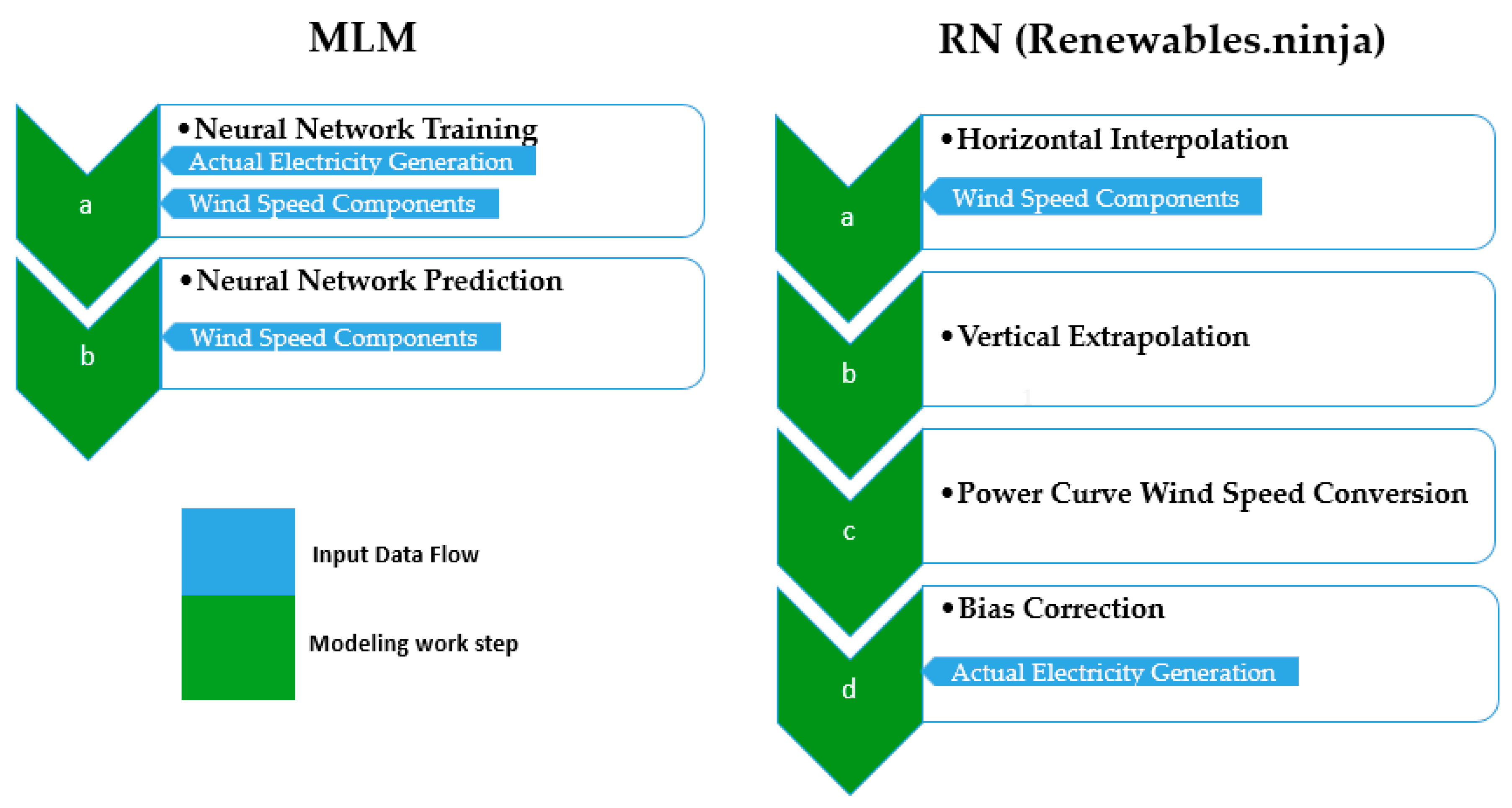
Figure 1 shows a brief comparison of our modeling approach and RN. In contrast to the rather simple ML modeling process, RN has to perform five major steps to derive a wind power time series. Our ML modeling process trains a neural network by regressing a set of predictor variables (wind speed components u, v and date dummies) on the response variable wind power generation (a) and uses the trained neural network to predict wind power generation by using a set of wind speed data from the same source but different time period and date dummy predictors (b) (
Figure 1). A more detailed description of the ML approach can be found in
Section 2.1.
In the RN approach, the following steps are taken (
Figure 1):
- (a)
Wind speed data were acquired, and wind speed components, i.e., the u and v variables, were interpolated from the MERRA2 grid to the actual turbine locations using LOESS regression.
- (b)
Wind speeds were extrapolated to the corresponding turbine hub heights from the three height levels provided by MERRA2 (2, 10, and 50 m above the ground) using the logarithmic wind profile.
- (c)
Wind speeds were converted to wind turbine power outputs by using manufacturers’ power curves.
- (d)
An additional bias correction step for calibrating results against actual electricity generation was performed in the RN model as a post-processing step.
A detailed description of the modeling approach used by RN can be found in Staffell and Pfenninger [
13]. In general, all power curve-based models follow a highly similar approach to RN.
Both our ML-based approach and RN used MERRA2 reanalysis as the data source for the 2, 10, and 50-m u and v wind speed components. We chose Germany as modeling location due to its highly developed wind turbine fleet, in addition to the sound availability of wind power generation data via the Open Power System Data (OPSD) platform [
35]. The model time period (2010–2016) was chosen to fit the longest openly available coherent time series of hourly resolved wind power generation. The temporal resolution of observed and modeled generations was hourly.
2.1. Detailed Description of MLM
Neural networks are commonly used algorithms for the short- and mid-term prediction of wind power generation [
25,
36,
37,
38]. In this study, we employed a multilayer perceptron neural network to regress climate variables and additional date dummies as predictor variables on the response variable, i.e., the actual wind power generation time series for Germany (
Table 1), to generate long-term time series of wind power generation.
To quantify how the quality of the ML-modeled time series depends on the extent of information about wind turbine locations, three neural networks MLM1, MLM2, and MLM3 were trained with three different input datasets. These datasets differed with respect to the amount of wind speed component grid points used (see
Section 2.2.1). The results of MLM2 and MLM3 do not differ strongly, results for MLM3 are therefore only shown in the
Appendix A.
The preparatory steps for the MLM approach consist of acquiring the necessary climate input data and deriving date dummy variables for MLM1. For MLM1, all climate data grid points within a bounding box around Germany are used. For MLM2, only data grid points close to actual wind power turbine locations were selected and for MLM3 climate data grid points have been further reduced based on the amount of installed capacity (see
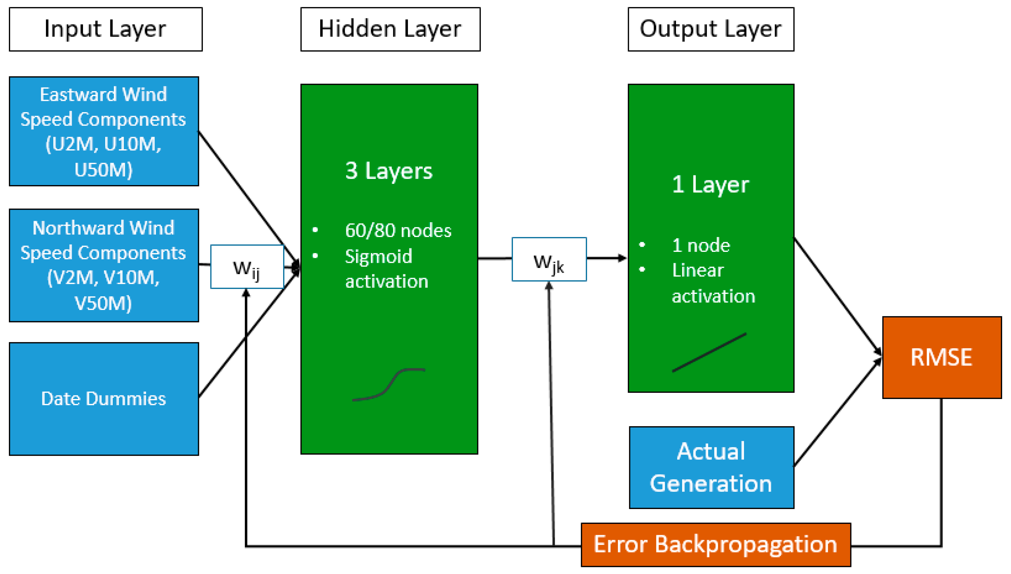
Section 2.2.1). Subsequently, the input data were applied to train the model on observed generation and, using that trained model, to predict generation for a period not used in the training of the model. In the first step, the neural network model parameters, i.e., the weights in the network, are estimated using the input data from the training period (training dataset). To guarantee reproducibility of results, we had pre-set the seed for the random number generator. The trained neural network is consequently fed with the remaining set of input variables (prediction dataset) to compute the modeled electricity generation from wind power for the prediction period in terms of capacity factors. We used a neural network with one input layer with a node size equal to the number of input predictor variables, i.e., our dummy variables and wind speed components; three hidden layers of a user-defined size; and one output layer of size one, i.e., electricity generation from wind power, which was the predicted variable. The activation functions used in the three hidden layers are of the sigmoid type and the output layer activation is a linear function. The neural network weights (i.e., w
ij and w
jk) were estimated by minimizing the error of the network output in comparison to observations. In the chosen neural network modeling framework, the Root Mean Square Error (RMSE) is the default error measure. Error backpropagation was used to minimize the error in an iterative process (
Figure 2). For the hidden layers, we tested models with layer sizes of 60 and 80 nodes. Out of these two models, the model size which resulted in better correlation, normalized root mean square error (NRMSE), and normalized mean absolute error (NMAE) was chosen for further use.
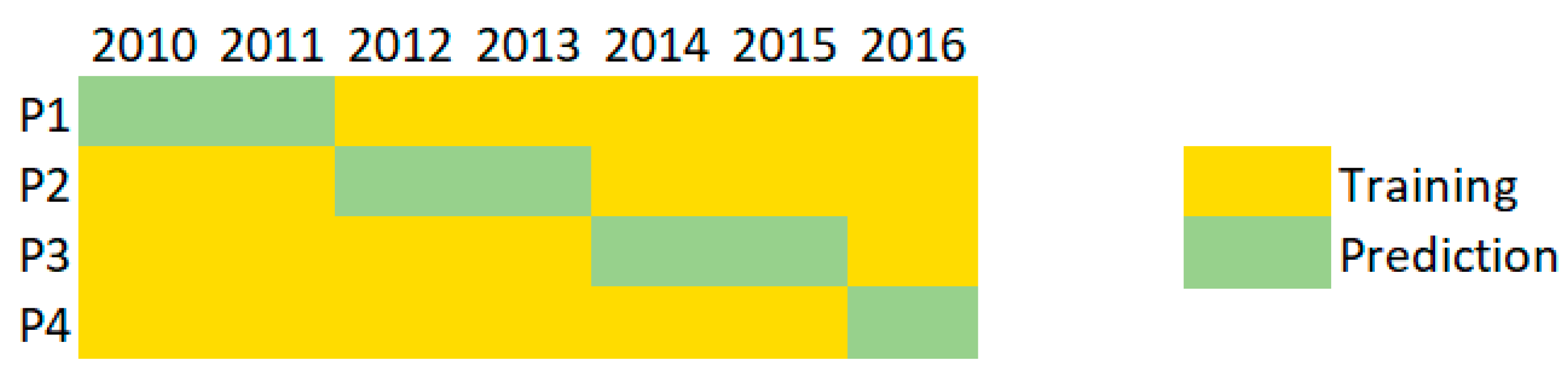
In order to reduce the number of model training iterations needed to generate the seven-year time series and to provide a sufficient time period for model training, the training time period needs to be rearranged for every prediction period. This results in four training and prediction iterations illustrated as P1–P4 (
Figure 3). For the prediction period of 2010 and 2011, the training period was set to 2012–2016. For the prediction period of 2012 and 2013, the years 2010–2011 and 2014–2016 were used for training, and similarly for all other periods. This resulted in a time series split between the training and testing period amounting to approximately 71 to 29% and ensured that every prediction was out-of-sample (
Figure 3).
Function calls and computations used for our ML approach were executed according to the specifications in Bergmeir and Benítez [
39] and the package documentation of the R-Package “caret” [
40]. The model training part consisted of a call to a training function, which resulted in a neural network model calibrated for estimating nationally aggregated wind power electricity generation based on wind speed and date dummy predictor variables. This neural network model was then used to derive an hourly wind power electricity time series solely based on out-of-sample predictor input variables.
All computations and visualizations were conducted in RStudio (Version 1.1.423) with R version “Microsoft R Open 3.4.3”. The packages “tidyverse”, “lubridate”, and “ggplot2”, and their corresponding dependencies were used for data handling and visualization. For model set up, training, and predictions, the package “caret” was used, which itself depends on the “RSNNS” package. Downloads and handling of MERRA-files were done with the R-package “MERRAbin” and its dependencies [
41]. The source code for this methodological approach and for the validation is available in a GitHub repository [
42]. The resulting ML-based time series have been made available as feather and CSV files on the hosting service Zenodo [
43].
2.2. Data
2.2.1. Climate Input Data
The present study is based on climate input variables from the global reanalysis data set MERRA2. This dataset was chosen to enable a comparison of our results and the time series from RN (ninja_europe_wind_v1.1-data package) [
34], which uses the same data source. The climate input data used in the MLM are featured in the time-averaged single-level diagnostics subset “tavg1_2d_slv_Nx”, whereby wind speed components U2M, V2M, U10M, V10M, U50M, and V50M, i.e., wind speeds at 2, 10, and 50 m above the ground, were used.
These variables for all MERRA2 grid points within a bounding box (longitude from 5 to 15.625, latitude from 46 to 56) around Germany constitute the input data set for the first MLM-generated time series (MLM1), where no variable subsetting was performed and all data points were used. The input dataset for the time series MLM1 did not feature any location information at all, which meant that all wind speed grid points in a bounding box around Germany were used. The input dataset for MLM2 contained implicit information on turbine locations via climate variable subsetting, which corresponds to using only the four wind speed grid points closest to locations where wind turbines were actually installed by 1 January 2017. This resulted in the use of all grid points within Germany plus some adjacent points. For MLM3, the set of grid points was further reduced to contain only those closest to an installed capacity above the third quartile of the capacity distribution in Germany and here no neighboring grid points are included opposed to MLM2 (
Figure 4). This subsetting is only possible when not only wind farm locations but also their installed capacities are known.
Therefore, the input datasets for MLM1, MLM2, and MLM3 only differ in the number of wind speed component values used (
Table 1).
2.2.2. Installed Capacity and Electricity Generation Data
The observed electricity generation from OPSD [
35] was used as the response variable for training the neural network for all MLM time series, as well as for assessing the quality of the modeled electricity generation time series.
These generation values were consequently converted to capacity factors (CF) by dividing them by daily values of the installed wind power capacity from OPSD [
35]. The locations and installed capacities of wind farms taken from OPSD [
44] were additionally used to spatially subset climate data by extracting wind speed components closest to the wind farm locations for MLM2 and MLM3. The installed capacity time series does not explicitly feed into either of the MLMs for reasons of comparability (RN time series are based on a single installed capacity value). Consequently, all variables were scaled by subtracting the mean and divided by the value range (minimum value subtracted from maximum value). Feature scaling is the standard procedure employed for reducing the computational effort in the training of neural networks. A list of all variables used in this study, in addition to their application, unit, size, and source, can be found in
Table 1.
2.3. Time Series Quality Assessment
Standard model error metrics (correlations and model error) and the modeled time series’ ability to replicate characteristics of the observed time series (distributions, seasonal characteristics, representation of extreme values, and power ramps) were assessed. The comparison is based on an hourly time series covering seven generation years (2010–2016). The time series quality was assessed for the whole seven-year time series. We emphasize here that we always compared the RN model to time series predicted from different trained models, i.e., we did not use training periods for comparison.
3. Results
In the results section, we present results of MLM1 and MLM2 in comparison to RN. The results of MLM3 are similar to MLM2 and are therefore shown only in the
Appendix A.
3.1. Model Selection
We tested two different network sizes—one with 60 and one with 80 nodes in the hidden layers—for generating the whole seven-year prediction time series with all considered models. The network size featuring better model error metrics was chosen for a more thorough assessment of the time series quality. When comparing error metrics for the two models MLM1 and MLM2 with a neural network of three hidden layers with 60 and 80 nodes each for the prediction period, MLM1 performs better with a smaller network size. MLM2 performs remarkably better when using the prediction dataset with the bigger network size (
Table 2).
3.2. Basic Time Series Quality
Both MLM time series feature comparable or better error metrics than RN. MLM2 also exhibits a similarly high correlation to RN.
The MLM1 hourly time series features a comparable NMAE (0.152), as well as a slightly lower NRMSE (0.209) value with a slightly lower hourly correlation (COR: 0.970), compared to the RN time series (NMAE: 0.152, NRMSE: 0.210, COR: 0.976). In comparison with the RN time series, the MLM2 hourly time series features a generally lower NMAE (0.138) and a lower NRMSE (0.191) value with a comparably high hourly correlation (COR: 0.975).
Both MLM1 (VAR: 0.025) and MLM2 (VAR: 0.025) estimate the total observed time series’ variance (VAR: 0.026) more accurately compared to RN (VAR: 0.030). When quantiles are considered, both MLMs are closer to the observed quantiles than RN, except for the 0% quantile where the MLMs are lower due to the presence of negative values, the 25% and 100% quantile for the MLM1 time series, and the 100% quantile for the MLM2 time series. The MLM1 time series features 53 negative capacity factor events and the MLM2 features 65 (
Table 3).
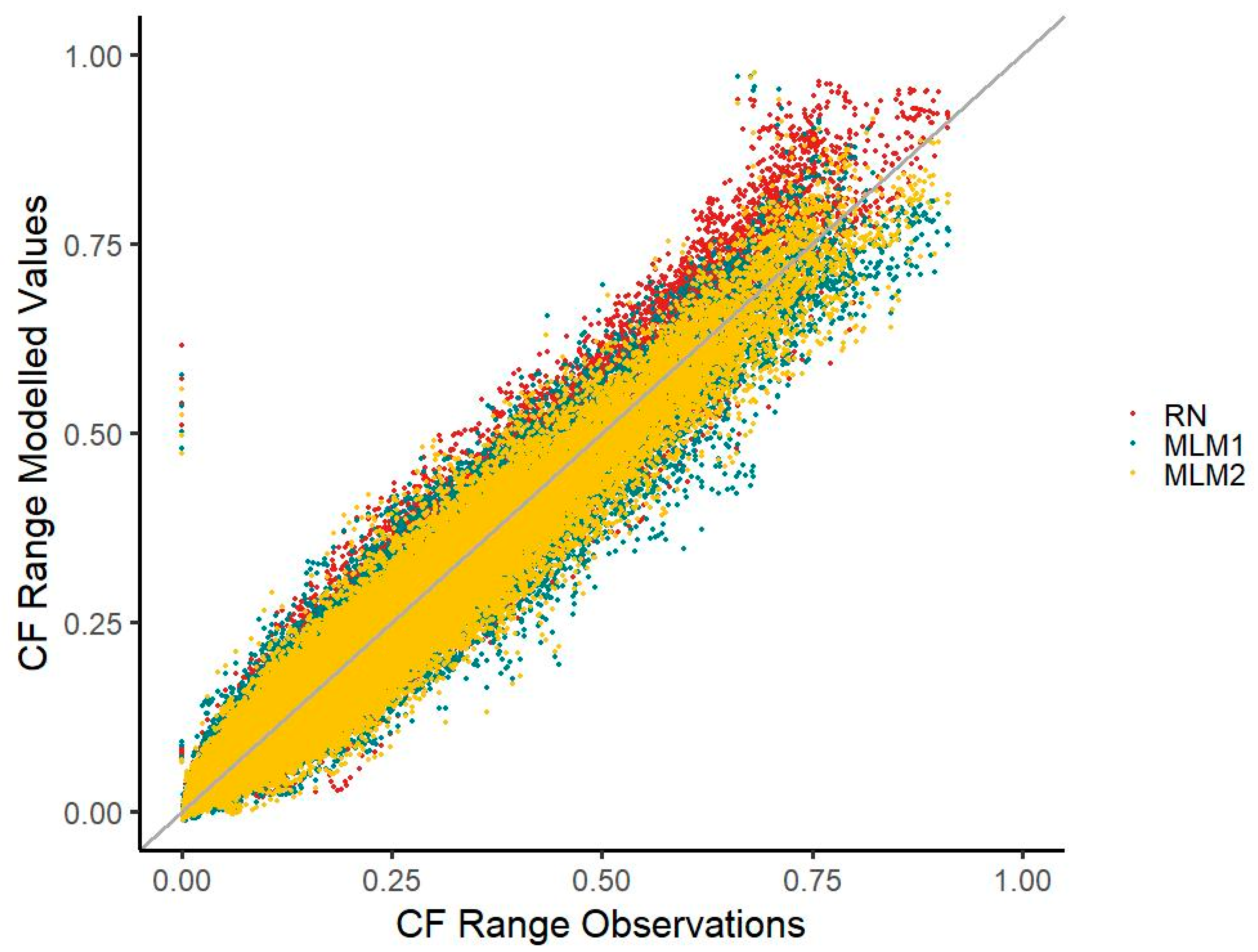
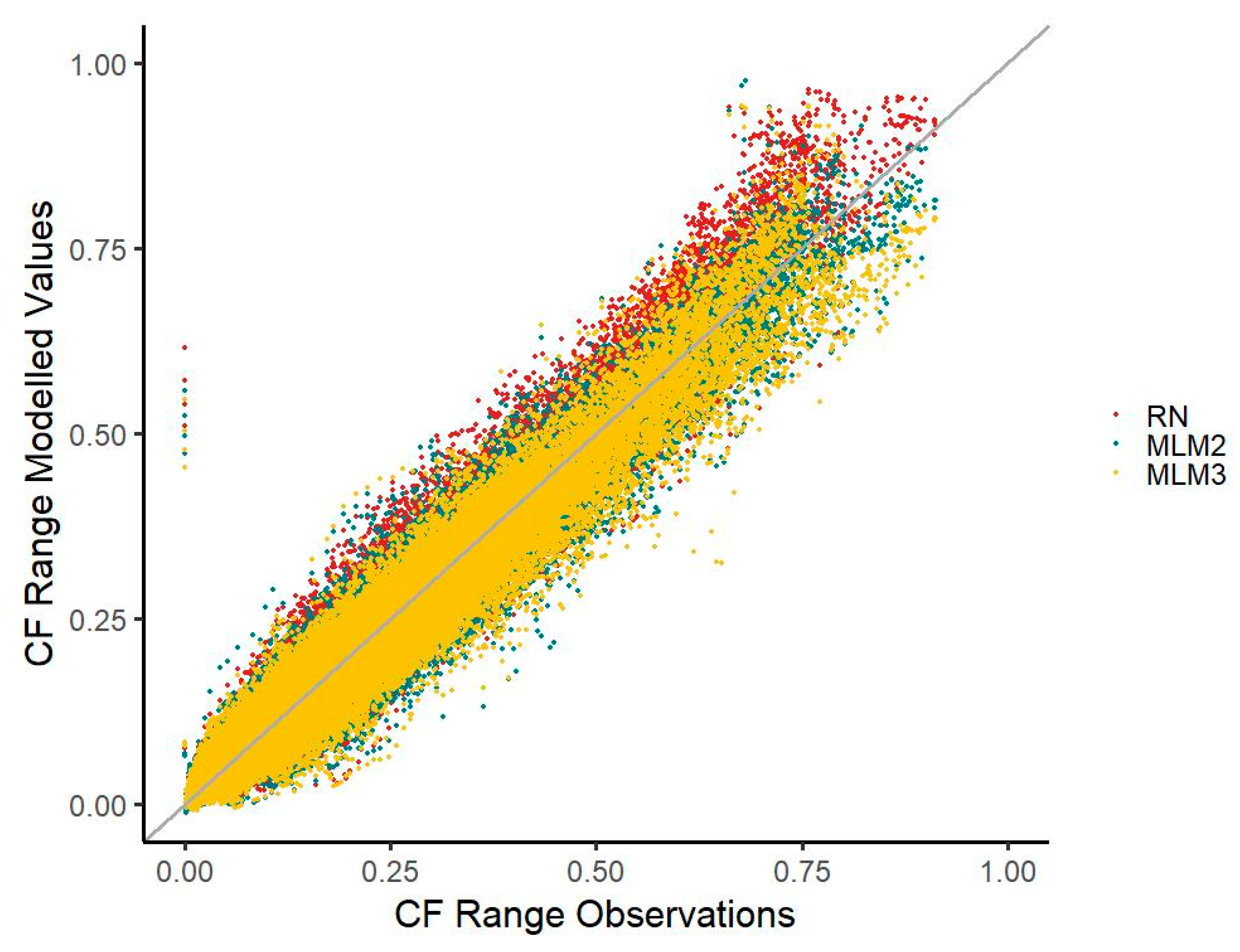
Except for the highest capacity factor (CF) range, both MLM time series mainly fare equally well to or better than the RN when deviations from observed values are considered.
Median deviations in five CF ranges (except for the CF ranges of 0.0–0.1, 0.4–0.5, 0.5–0.6, and above 0.8) are less distant to zero when compared with the MLM1 time series. With the MLM2 time series, the median deviation for five CF ranges is less distant to zero than that of the RN time series (except for the CF ranges of 0.0–0.1, 0.3–0.4, 0.4–0.5, and above 0.8). With the RN time series, an overestimation is apparent in the scatterplot, particularly in the higher CF spectrum. The ranges of deviations for MLM1 are slightly wider than those of the RN time series, except for the values of 0.0–0.1, 0.1–0.2, and 0.2–0.3. In a similar way, the deviation ranges of MLM2 are only narrower than the RN deviations in two CF classes (CF 0.0–0.1 and CF 0.1–0.2). The deviation median in the MLM2 time series is generally less distant to zero than in the MLM1 time series, except for the CF classes of 0.2–0.3 and 0.3–0.4. For the deviation ranges, the picture is fairly the same, with the MLM2 time series featuring a narrower range in five CF ranges (0.0–0.1, 0.4–0.5, 0.5–0.6, 0.6–0.7, and 0.7–0.8). This is also reflected in the scatterplot with the MLM2 values more concentrated towards the diagonal line than the MLM1 values. Both MLM time series also mainly underestimate generation slightly within most CF classes, whereas the RN time series overestimates generation (
Figure 5).
The MLM1 and MLM2 time series reduce the underestimation of CF values around 0.1 visible in the RN time series. However, both MLMs underestimate the occurrences of CFs in the very low range compared with RN.
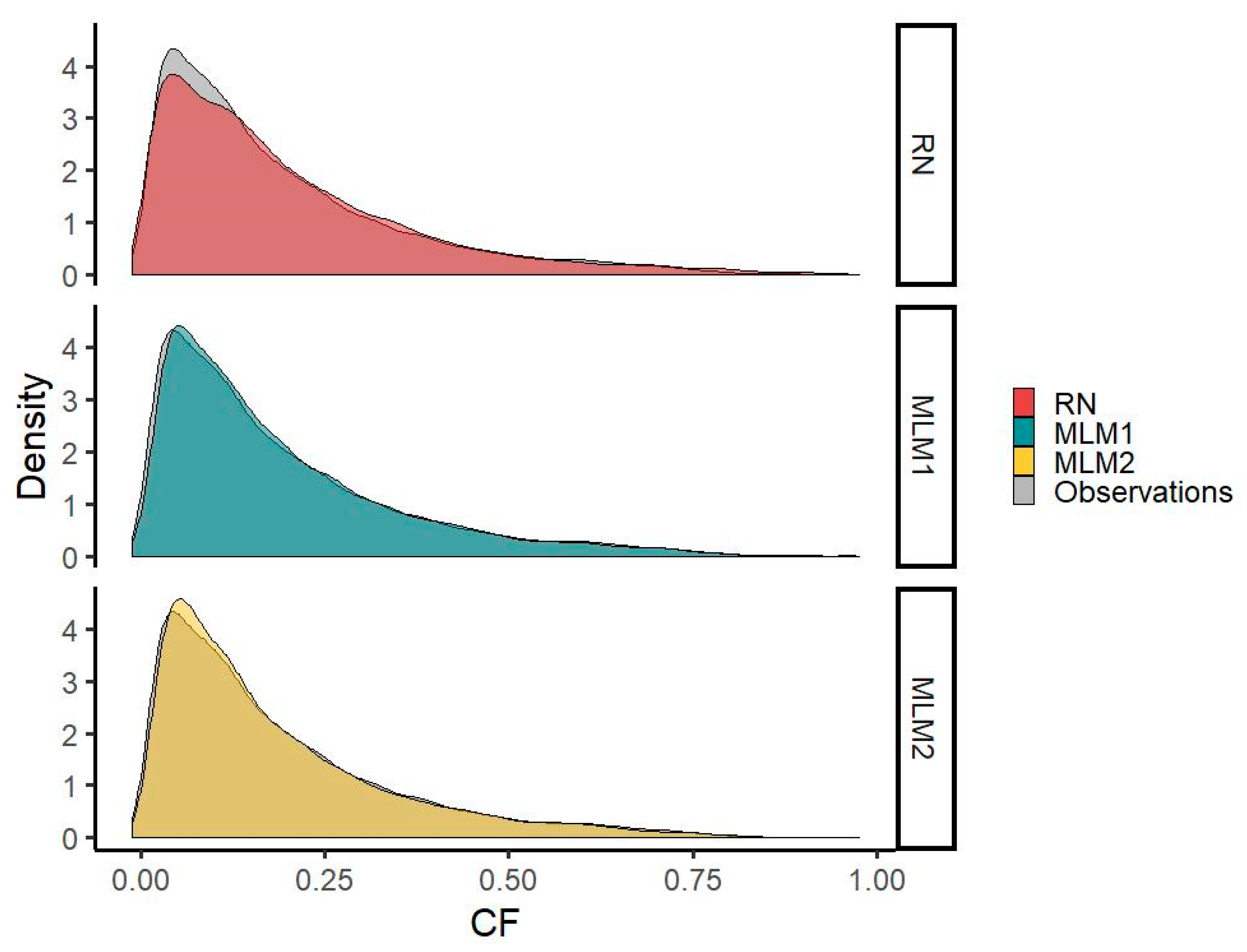
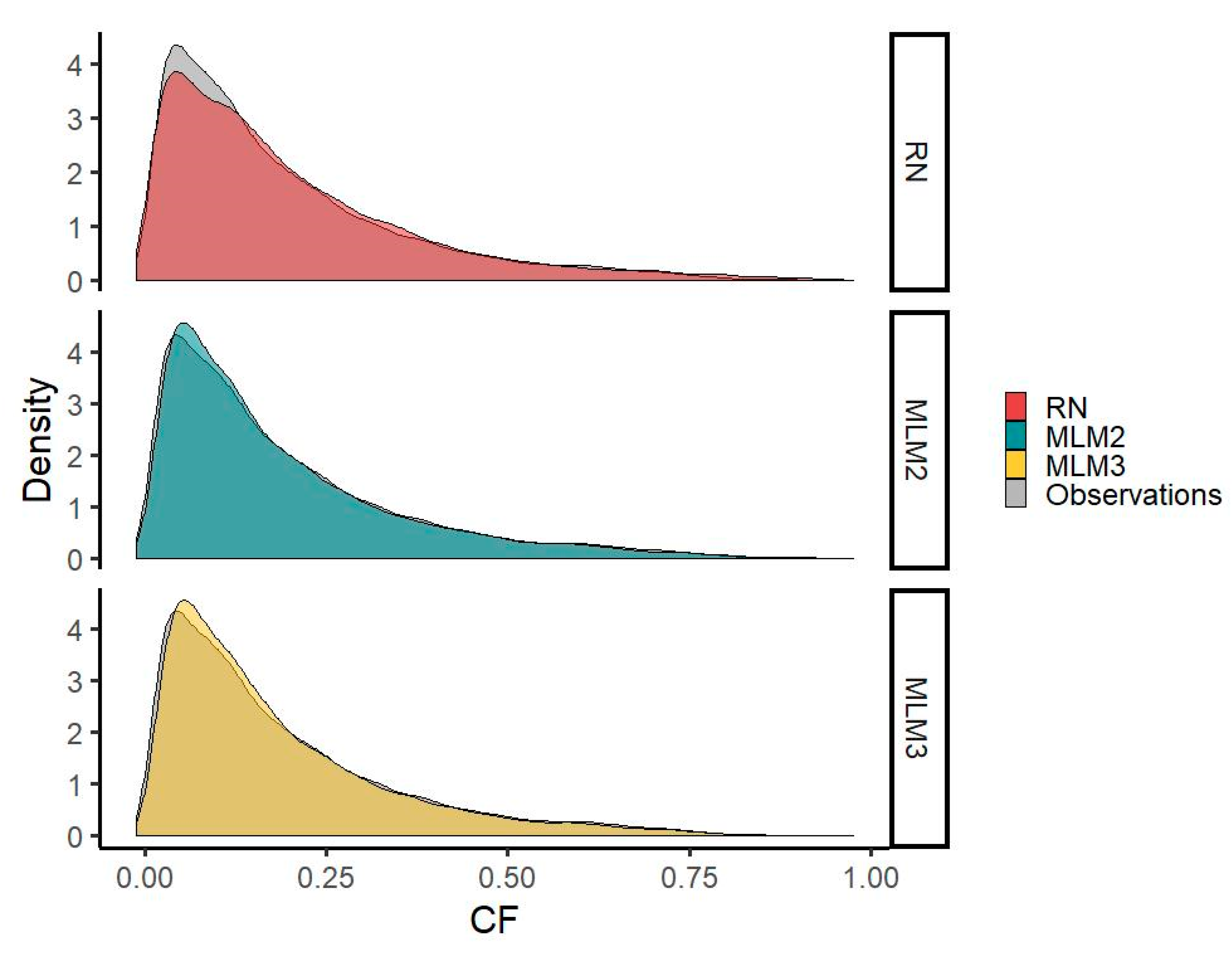
The results show an acceptable representation of the distributional characteristics of the observed time series comparable to the results of RN for both MLM time series. Generation in the very low CF range (8254 actual values with a CF < 0.04) is better approximated by the RN time series (8138 modeled values with a CF < 0.04) than by MLM1 (6658 modeled values) or MLM2 (7115 modeled values) time series, which is also represented by a higher density in the RN time series. CFs in the range around 0.1 (8928 actual values between 0.08 and 0.12), where an overestimation occurs in the MLM-derived time series (9146 modeled values for the MLM1 time series and 9249 for MLM2) opposed to an underestimation in the RN time series (7989 modeled values), however, are better represented by the MLMs. This can also be seen by a better fit of the probability density curve in this range for both MLMs. In the high CF range, the frequency of CF values above 0.8 is, although slightly underestimated (75 and 126 values > 0.8 for the MLM1 and MLM2 versus 121 actual values), better approximated by the MLM time series than by RN (471 modeled values > 0.8) (
Figure 6).
3.3. Diurnal Characteristics
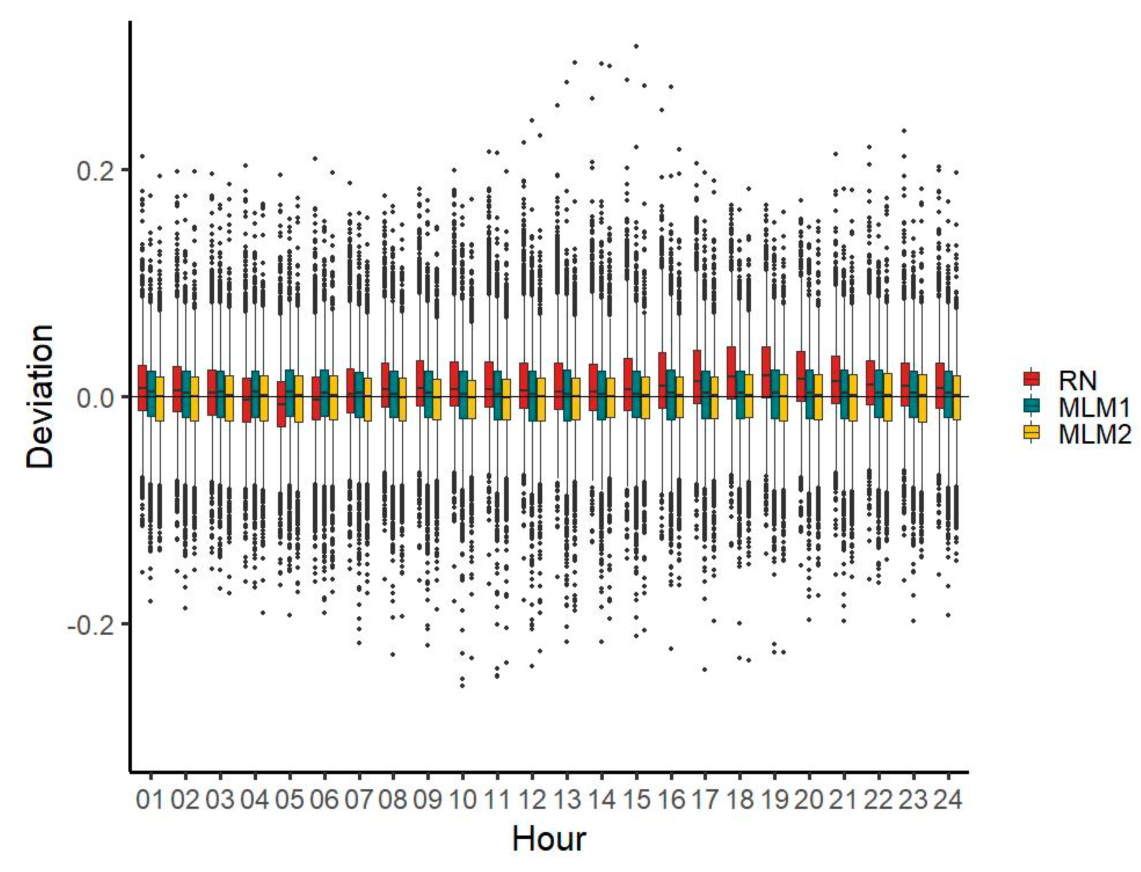
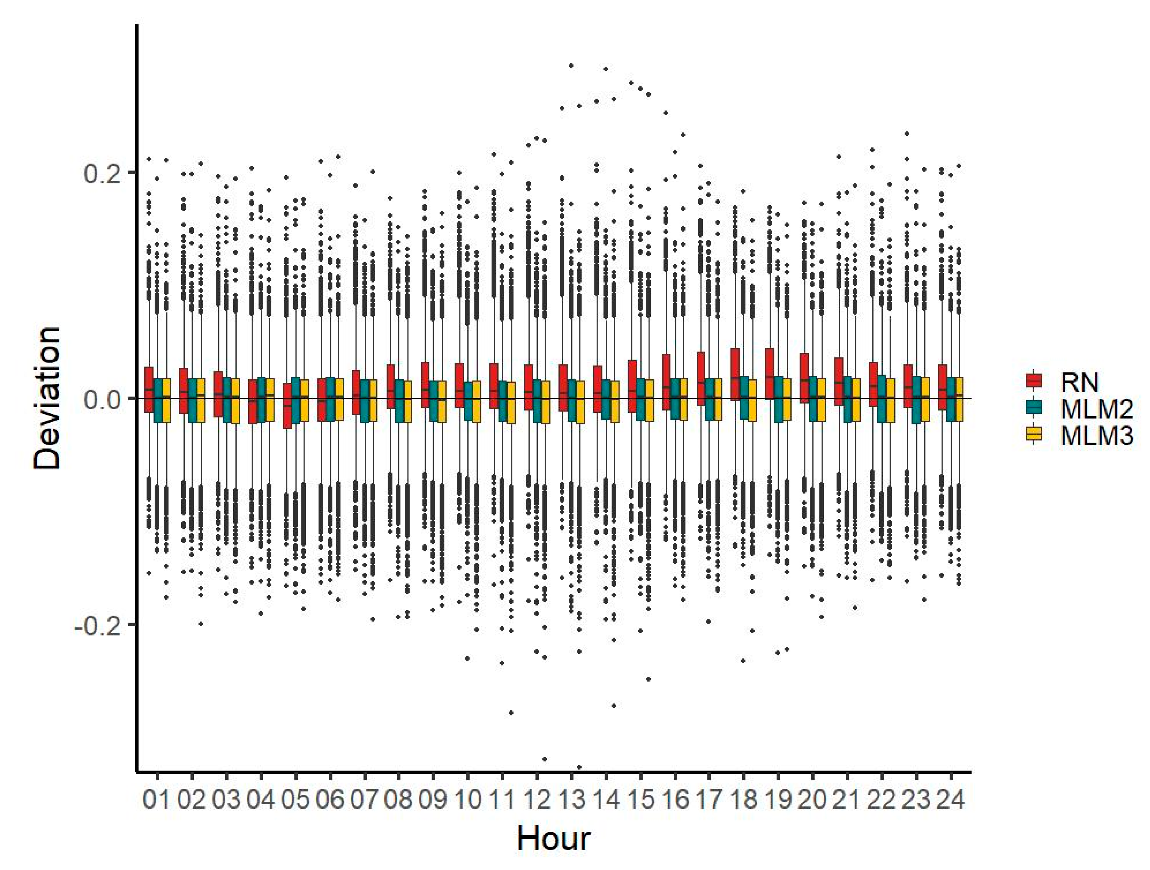
MLM2 provides a better estimate of diurnal characteristics for most hours and both MLM time series reduce deviations in the evening hours featured in the RN time series (
Figure 7).
RN median deviations are generally lower than those of MLM1, except for seven hours (hours 2, 15, 16, 17, 18, 19, and 20). For MLM2, the median deviations are generally lower than those of the RN time series, except for four hours (hours 4, 6, 22, and 23). For RN, the mean of deviations is highest around the evening (hours 18, 19, and 20), where it is noticeably higher than during the rest of the day. It is lowest during the morning (hours 7 and 8) and around midnight (hours 1 and 24), where it is lower than during the remaining hours. The MLM1 and MLM2 time series do not feature a similarly strong increase of the deviation median in the evening hours.
The deviation range of the MLM1 time series is narrower for 8 h (hours 1, 2, 3, 4, 5, 6, 22, and 23) compared with the RN time series, and for 12 h (hours 1, 2, 3, 4, 5, 6, 7, 9, 21, 22, 23, and 24) when compared with the MLM2 time series. For all three time series, the deviation range is remarkably wider in the early morning hours 2–5 than during the remaining hours. With all three time series (most remarkably with the MLM1 time series), an increase of the deviation range around noon and early afternoon can be seen and for all three time series, the deviation range decreases again for the evening hours (
Figure 7).
3.4. Seasonal Characteristics
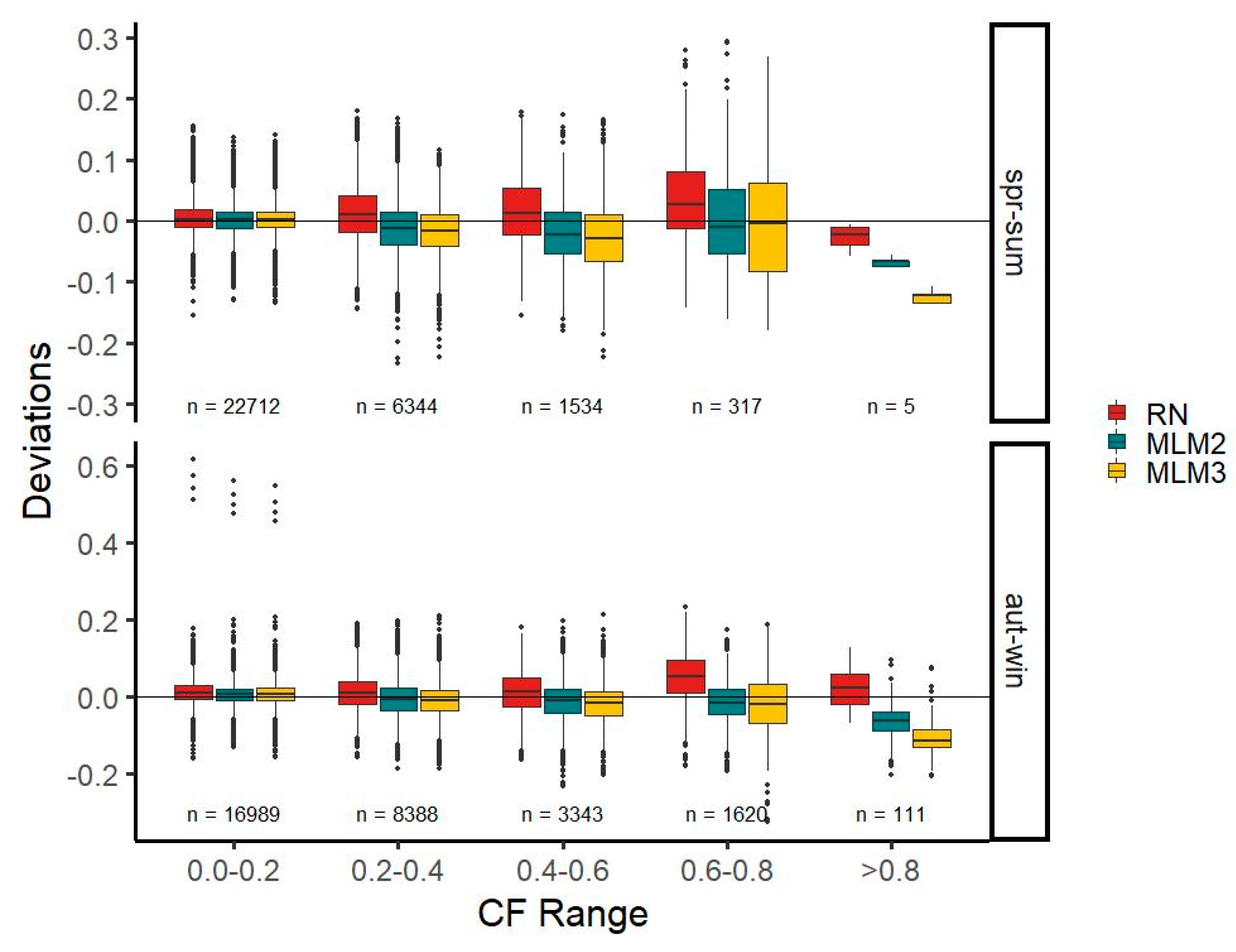
Here, we split all three time series into an autumn-winter and a spring-summer half-year to compare seasonal characteristics. March, April, May, June, July, and August constitute the spring-summer half year, and the remaining months comprise the autumn-winter half-year. RN, MLM1, and MLM2 reflect seasonal characteristics comparably well (
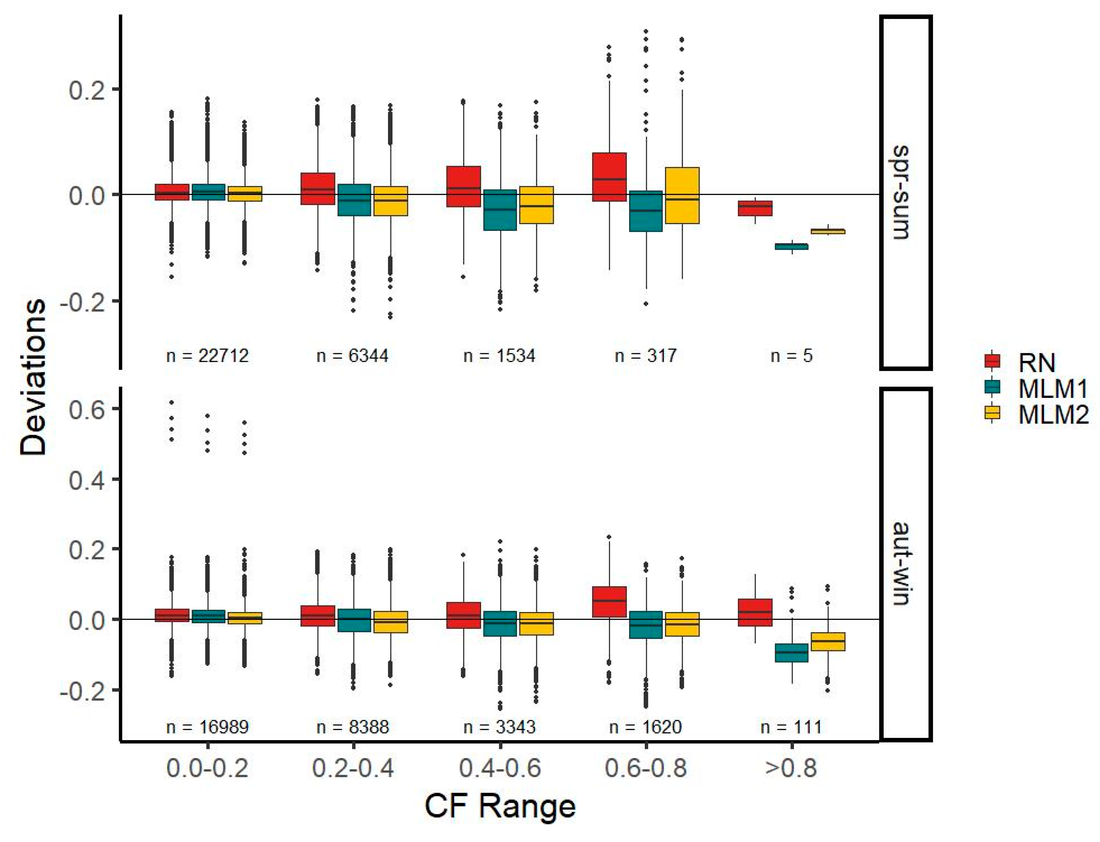
Figure 8). However, MLM2 performs better than MLM1 in the majority of CF classes. Interestingly, the lowest CF class in the autumn-winter half-year features four outliers in all three time series.
When comparing observations made with the MLM1 time series, the median deviation is lower than for RN for three out of 10 CF classes, where MLM1 is better in the CF classes 0.0–0.2, 0.2–0.4, and 0.6–0.8 in the autumn-winter half-year. The MLM2 time series performs better in four out of 10 CF classes—the same classes as MLM1—and in the 0.6–0.8 class for the spring-summer half-year. This means that the RN time series fares better than both MLM time series in a seasonal comparison; however, for most classes, only by a small margin. For all three time series, a tendency to overestimate values in the lowest CF class can be observed. In the remaining CF classes, the MLM time series mainly underestimate, whereas the RN time series overestimates. In the comparison of the deviation ranges (spread from the minimum to maximum deviation value), MLM2 fares equally well as MLM1, outperforming the RN time series in four out of 10 classes. Both MLMs perform better than RN in the class 0.0–0.2 in both half-years, in the 0.6–0.8 class for the autumn-winter half-year, and in the >0.8 class for the spring-summer half-year. Remarkably, the lowest class in the autumn-winter half-year features some outliers, skewing all three time series towards a high deviation range. For the deviation mean, MLM2 outperforms RN in more CF classes than MLM1 (
Figure 8).
3.5. Durations and Frequencies of Low, High, and Extreme Values
MLM1 and MLM2 provide a better estimate of frequencies and durations of low CF extremes and frequencies of high CF extremes. Durations of high CF extremes are better approximated by RN.
Frequencies (102 actual events) of low-capacity factor extreme values (CF < 0.005) are better approximated by MLM1 (193 modeled events) and MLM2 (238 modeled events) than by the RN time series (430 events), where both MLMs provide a less pronounced overestimation and therefore better approximation. The mean durations (3.19 consecutive hours of observed generation below 0.005 CF) of the low-capacity factor extreme values are also better approximated by MLM1 (3.27 consecutive hours of modeled generation below 0.005 CF) and MLM2 (3.50 consecutive hours of modeled generation below 0.005 CF) compared with RN (4.62 consecutive hours of modeled generation below 0.005 CF). Both MLM time series provide an exact match of the low generation extreme maximum duration (10 observed consecutive hours below 0.005 CF), whereas the RN time series overestimates the maximum duration (14 consecutive hours of modeled generation below 0.005 CF). Frequencies (121 actual events) of high-capacity factor extreme values (CF > 0.8) are better approximated by MLM1 (75 modeled events) and MLM2 (125 modeled events) than by RN (471 modeled events). When mean durations of very high generation events (7.56 observed consecutive hours) are considered, RN (9.24 modeled consecutive hours) provides the best estimate compared with MLM1 (4.17 modeled consecutive hours) and MLM2 (5.21 modeled consecutive hours). With regard to the approximation of maximum durations (35 consecutive observed hours), the MLM1 time series (11 modeled consecutive hours) is fairly far off, whereas RN (33 modeled consecutive hours) and MLM2 (21 modeled consecutive hours) provide better estimates (
Table 4).
3.6. Frequencies and Ranges of Power Ramps
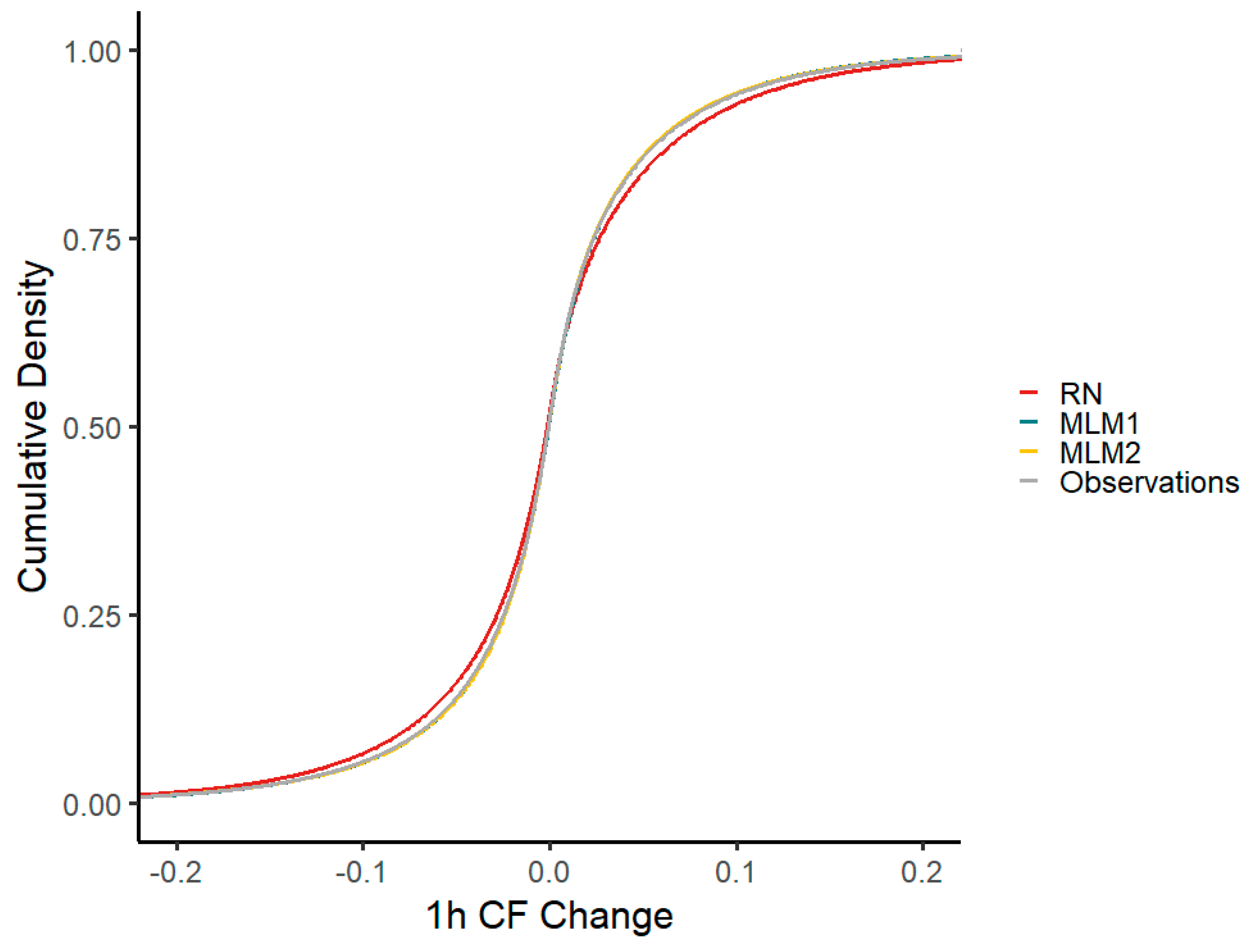
Both MLM time series follow the cumulative density of capacity factor changes within one hour better than the RN time series. In particular, the RN time series overestimates the density within the range of negative CF changes between −0.1 and 0 and underestimates it within the range of positive CF changes between 0 and 0.1. MLM1 and MLM2 do not show this behavior and nearly match the observed CF change density exactly (
Figure 9).
Within all considered time frames, both MLM time series replicate CF changes better than or equally well to the RN time series. CF changes within four different time frames (1, 3, 6, and 12 h) are better than or equally well replicated with MLMs compared to RN. Both MLM time series feature mean values of positive and negative CF changes, frequencies of negative and positive CF changes, minimum and maximum ramp values, and an approximation of the frequencies of fairly high and low power ramps comparable to or better than the RN within nearly all time frames. All models fare better the longer the time frame, reflecting the ability of the reanalysis data source to replicate the temporal variability of wind speeds within longer time frames (
Table 5).
4. Discussions
The MLM approach can only be successfully applied if (1) sufficiently long and high-quality climate input data and generation data are available for the prevailing wind conditions and turbine locations in a region, which is currently not the case for all regions. This, however, does not translate to a downside of using a neural network approach as this also holds true for power curve-based models, which need observations for calibration or validation. (2) The MLMs are not capable of reflecting changes in the spatial configuration of the installed wind turbine capacity as installed capacities are not used as model inputs. However, the proposed approach can be easily adapted to make use of information on installed capacities. (3) The applicability of wind power models is quite diverse. Therefore, the scope of this study was limited to a comparison of the time series quality for RN and the proposed MLM approach. The advantages and disadvantages of using one method over the other can be different, depending on the application; however, a large difference in impact between using a power curve-based or MLM-derived one is not to be expected based on the comparison of time series quality. The proposed approach of deriving time series by means of neural networks is only (4) partly suited to generating future scenarios taking significant technological developments into account (e.g., a considerable shift of the ratio between the rotor diameter and installed capacity, such as in turbines specifically designed for low wind speed conditions) compared with a power curve-based approach such as in RN. Using turbine specifications as an input to model training can probably compensate for this downside in subsequent model iterations, although this would require additional technical information on the turbine types used. (5) Landmark changes in technology (e.g., horizontal turbine design) or the regulation of wind turbines or intermittent renewables (e.g., increased curtailment) in general, for which no observational data are available, cannot be successfully replicated by the proposed neural network approach. This issue can be addressed for both methodologies using post treatment of the model output. (6) For the MLM training step, a significant amount of computational effort is required, which is potentially higher than the computational effort associated with the model setup of power curve-based models. The prediction step, however, is comparable in computational complexity to power curve-based approaches.
5. Conclusions
All three machine learning models were able to generate wind power generation time series comparable to or even better than a state-of-the-art power curve-based modeling approach (Renewables.ninja, abbreviated as RN) with respect to standard error metrics, seasonal and distributional characteristics, and frequencies and durations of low, high, and extreme values, as well as for the replication of frequencies and durations of power ramps for wind power generation.
We used three datasets—one without location information, and two with implicit location information via incremental climate data grid point subsetting—as the input for MLMs to assess whether location information is needed to obtain a time series quality comparable to that of RN. We found that (1) all three input datasets for the machine learning model time series were able to generate wind power generation time series comparable to or even better than a state-of-the-art power curve-based modeling approach (RN) with respect to the quality measures considered. (2) Furthermore, the information required for model setup with regard to knowing accurate wind turbine locations and power curves is much lower. The additional information on turbine locations and the used turbine models is not strictly needed to reach a time series quality comparable to that of the RN approach, although implicit location information improves most of the time series quality measures considered as MLM2 and MLM3 outperform MLM1 in most cases. This translates to less spatial information on installed capacities being required when using the ML-based approach, while still attaining a time series quality similar to RN. (3) All MLM-generated time series (especially MLM2 and MLM3) additionally show a reduced overestimation of very high CF values and reduced underestimation of CF values around a CF of 0.1. (4) The time series quality varies, depending on which quality parameter is considered and on which MLM is used. However, there are no major drawbacks of using a machine learning approach for the purpose of generating wind power time series, with the exception of the duration of high generation extreme events, which are rare. (5) The presence of negative CF values indicates that longer training periods could be helpful as the whole range of all input variable combinations and thus, the variability of climate data has not been fully captured by the available training time frames. However, negative values can easily be handled via simple post-processing.

 ,
, 


