Article

An MPC Approach for Grid-Forming Inverters: Theory and Experiment

by
Alessandro Labella
1,
Filip Filipovic
2,
Milutin Petronijevic
2,
Andrea Bonfiglio
1,* and
Renato Procopio
1
1
Department of Electrical, Electronic, ICT Engineering and Naval Architecture, University of Genoa, I-16145 Genova, Italy
2
Faculty of Electronic Engineering, University of Niš, 18000 Niš, Serbia
*
Author to whom correspondence should be addressed.
Energies 2020, 13(9), 2270; https://doi.org/10.3390/en13092270
Submission received: 17 March 2020 / Revised: 17 April 2020 / Accepted: 23 April 2020 / Published: 4 May 2020
(This article belongs to the Special Issue Dynamic Modeling of Microgrids)

Abstract

:
Microgrids (MGs) interest is growing very fast due to the environment urgency and their capability to integrate renewable energy in a flexible way. In particular, islanded MGs in which distributed energy resources (DERs) are connected to the infrastructure with power electronic converters have attracted the interest of many researchers of both academia and industry because management, control and protection of such systems is quite different from the case of traditional networks. According to their operation mode, MGs that power electronic converters can be divided into grid-forming, grid-feeding and grid-supporting inverters. In particular, grid forming inverters are asked to impose voltage and frequency in the MG. This paper aims to propose a model predictive control (MPC) based approach for grid-forming inverters in an islanded MG. The MPC strategy is implemented because of its capability to define the optimal control actions that contemporarily track the desired reference signals and accounts for equality and inequality constraints. The overall problem formulation (objective function and relevant constraints) is described step by step and considers the specificity of the considered DC source. The proposed approach allows for the obtaining of very good results in terms of readiness against disturbances, even if it requires being fed only by local measurements. In order to validate the developed method, this paper proposes an experimental validation of the designed MPC controller in order to show its correct operation on a real system in a power hardware in the loop set-up using a rapid control prototyping approach.

1. Introduction

The interest in microgrids (MGs) is growing very fast as they represent a possible solution to a complete integration of renewable energy sources (RES) thanks to their flexibility [1,2,3]. The massive number of energy sources connected to the grid through power electronics converters is changing the classic paradigm of the electric power systems [4,5]. This evolution claims for new strategies to ensure power-sharing [6], voltage and frequency control [7] and grid support [8,9].
Inverters that interface distributed energy resources (DERs) to the MG can be classified according to one of the three following operation ways: grid-feeding, grid-forming and grid-supporting power converters [10,11,12].
Grid-feeding converters are designed to supply a specified value of active and reactive power. This operation allows for the considering of the controlled DER as an ideal current source connected to the grid in parallel with high impedance.
Grid-forming converters can be represented as an ideal AC voltage source with a low impedance in series, defining the frequency of the MG and the voltage amplitude at its terminals.
Finally, grid-supporting converters can be either seen as a current or voltage sources in which the current (voltage) is selected according to specified control laws (e.g., droop characteristic [13], voltage/reactive power control curves [14,15], active power/reactive power characteristic [14,15] and so on). Figure 1 schematically represents these operation modes.
The traditional control scheme for a grid-forming converter can be found in Figure 2. It is composed of two internal loops regulated by proportional-integrator (PI) controllers [16]. In this control scheme, the amplitude of the voltage at the point of common coupling (PCC) and current are measured and transformed in the dq reference frame by applying the park transformation and comparing to reference values as shown in Figure 2. According to Figure 2, V* represents the AC voltage reference at PCC, vd* and vq* are its d and q components, respectively, while vd (vq) is the measured direct (quadrature) axis voltage; id (iq) is the measured direct (quadrature) axis current and id* (iq*) is the corresponding reference; finally Ud (Uq) is the d (q) component inverter AC side voltage.
The current trend in developing new grid-forming strategies is to emulate the behavior of a traditional synchronous generator, indeed in that way it is possible to (i) simplify their integration in MG providing virtual inertia and/or to (ii) bring them to behave as similar as possible to something that is well-know and spread [17]; thus it results in the so-called virtual synchronous machine (VSM) control strategy. Converters managed with this kind of control can be used both in island and connected MGs. These strategies use the measurement of the AC variables to detect disturbance, voltage drops or frequency deviation and, through suitable command laws implemented in their own control, make the inverter mimic the synchronous machine. Since VSMs are very flexible, the authors of [18] proposed and verified an approach to mitigate voltage and frequency deviations in MG with synchronous generators. In [19], VSM and droop control dynamics are compared to exploring swing equations. In [20], the authors propose a control strategy in which, using an internal model for the harmonic oscillator, the converter dynamic results increased and exactly matched with the synchronous machine one.
Another important control family is composed by controllers that use sliding mode control to improve the transient response [16], applying it in for the inner current control loop [21,22].
Model predictive control (MPC) is also used with success in many fields of applications [23] thanks to its ability to manage multi-objective optimization problems in constrained systems. In [24], authors propose an MPC regulator able to optimize energy and power flows between MGs. In [25], an energy management optimization based on a distributed MPC is proposed; then in [26] a centralized MPC regulator for dynamic optimal power flow between energy storage systems is developed. Finally, MPC has also been used to ensure power grids transient stability [27]. Paper [28] proposes an MPC primary regulator for islanded MGs to control the output voltage of each inverter; instead, in [29] MPC is exploited with sliding mode (SM) to control the inverter output voltage and to limit the current in overload scenarios. Another interesting use of MPC for MGs voltage control is described in [30] where a distributed MPC control is proposed, in which each unit solves its own cost function. Reference [30] proposes a new way to implement secondary control for voltage restoration but there is no novelty for primary control (a simple droop logic is used) and there is no possibility to avoid communication among the units.
Another MPC based approach is provided in [31] where the traditional MPC is coupled with a finite control set MPC, a strategy very common in the power control field, in order to improve the stability and to reduce the total harmonic distortion. An alternative interesting development is provided by [32], in which four MPC implementations are proposed. In this frame, MPC is used with a minimal prediction horizon (one step forward), in fact MPC is used just to provide a better estimation of voltage measurement; it acts similarly to a feedforward compensation. For this reason, the cost function has a very simple formulation
The present paper aims at adopting the MPC control strategy to make the inverter behave like an ideal voltage source (grid-forming mode). This is normally done using conventional PI controllers; however, in this case the physical limitation of the converter itself (e.g., maximum current limitation) can be only imposed by means of a saturation in the inner current control loops (see Figure 2). Consequently, when the outer voltage control loop asks for unfeasible currents, the inner loop opens, which means that the overall control scheme is not able to track the voltage reference. Furthermore, the presence of two nested control loops makes the design of the controllers quite cumbersome. In the conventional strategy, there are four PI controllers (direct and quadrature axis voltage and current regulators), which means that there are eight parameters to be set. To the best of the authors knowledge, such choice is typically made by an empirical procedure that must ensure that the dynamics of the outer voltage control loop is much slower than the current controllers one.
On the other hand, the proposed approach allows to impose equality and inequality constraints; so, the controller selects the best control law that respects all such constraints. Furthermore, the only parameters to be set are the weights in the objective function that, as will be clarified later on, are only three and they can be selected independently of each other and represent the strength of the controller to track the reference values for the AC voltage and the system inputs (i.e., the inverter modulating signal frequency and the time derivative of the modulation index).
From a practical standpoint, the proposed MPC approach shall provide a more performing operation of a grid-forming inverter reducing at minimum the condition of maloperation due to the limitation of the converter and providing better time responses thanks to the model-based feature of the MPC technique. Of course, this improved performance requires an increased CPU effort; to check whether it is consistent with available computational resources, an experimental validation of the proposed strategy is presented to highlight the elements to be taken into consideration for a real control implementation and test the effectiveness of the proposed approach.
Experimental results have been obtained thanks to a rapid prototyping system (RPS) located at the laboratory for electric drives at the University of Niš, Serbia. Such RPS uses the dSPACE (DS1103, dSPACE, Paderborn, Germany) environment that allows for the exchange of input and output between on-field devices and the PC.

2. Some Remarks about the MPC Technique

Consider the following time-invariant-affine discrete time system:
x k + 1 = A x k + B u k + f
where x k n   and u k m represent the states and inputs, respectively, at time kTs, being Ts the sampling time. The MPC regulator acts to control the states of the system to a reference value xref by computing the solution of the following constrained quadratic programming (QP) problem:
min U e k + N T Q e k + N + i = 0 N 1 e k + i | k T Q e k + i | k + u k + i T R u k + i
s . t . x k + i + 1 | k = A x k + i | k + B u k + i | k + f
H u u k + i K u , i = 0 , , N 1
H x x k + i K x , i = 0 , , N 1
where ek is the state vector error, xk + 1|k refers to the prediction of the state at time (k + 1)Ts calculated at time kTs and N is the prediction horizon, i.e., the number of samples taken into account in the forecast. U = [ u k T u k + N     1 T ] T is the vector containing the optimal input vector uk, while Q = QT, R = RT are symmetric and positive semi-definite weighting matrices. Hu, Ku, Hx, Kx are the matrices that define the constraints for the controlled system. The MPC controller generates the control action using this strategy: at each step the control solves the optimization problem (2), predicts the evolution of the state variables based on their current values and calculates the optimal input for the system within the control horizon. Then, only the first step uk is applied to the system while the rest of the solution is just discarded. The process is then repeated: a new prediction of the evolution of the states is calculated based on the measurements of their current value, and another set of optimal control action is produced (Figure 3).
If the considered model is not linear, at any sampling step kTs a linearization procedure around xk is required to obtain the system described in (1). More details can be found in [33].

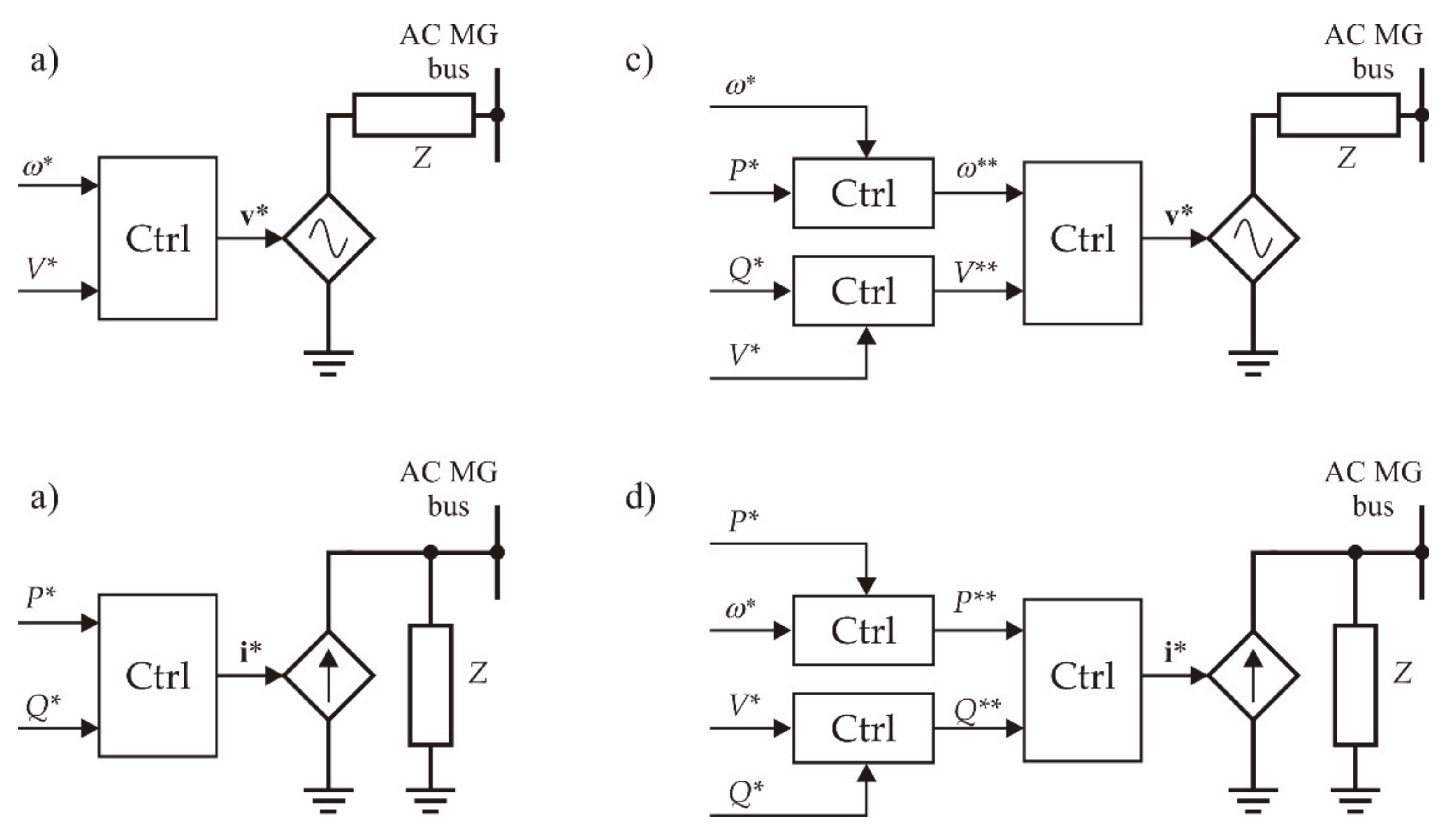
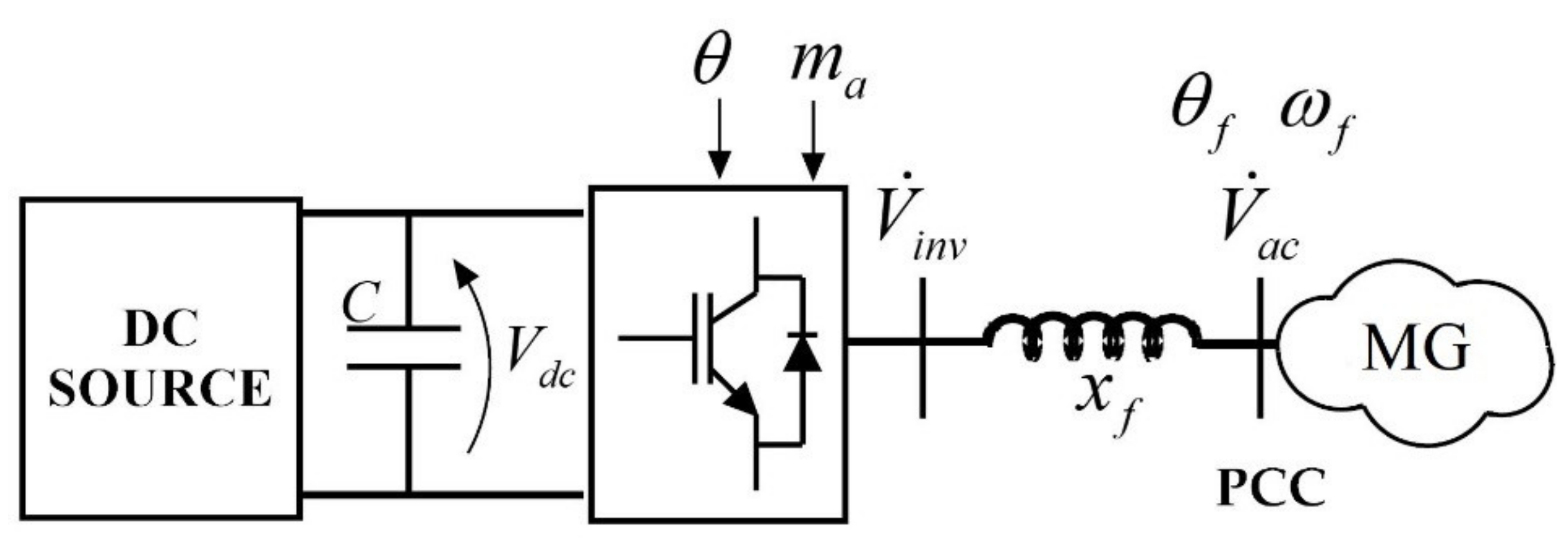
3. MPC Controller Design for Grid-Forming Inverters

The aim of the proposed MPC controller is that of providing a decentralized control of the MG and thus the control needs to be implemented without knowing the MG topology and parameters and relying only on local measurements.
Let’s consider a generic distributed generator (DG) as depicted in Figure 4. It consists of a generic DC source, a DC link with suitable DC filters, a full IGBT bridge inverter, an AC filter and finally a PCC.
In order to perform the design procedure for the MPC controller, it is necessary to define a mathematical model for the controlled system. Such a model is here proposed according to the following assumptions [34,35]:
  • AC side of the MG is supposed to be at steady state while DC dynamics are fully considered;
  • Higher-order harmonics are neglected;
  • DC inductor is neglected;
  • The shunt section of the AC filter is neglected.
The resulting model, represented in Figure 5, has been extensively validated with experimental measurements, as detailed in [35].
The phasor of the line-to-ground voltages at the inverter output V ˙ i n v t and at the harmonic-filter output V ˙ a c t can be respectively written as:
V ˙ i n v t = m a t V d c t 2 2 e j θ t
V ˙ a c t = V a c ( t ) e j θ f t
where ma is the inverter modulation index, Vdc is the DC link voltage and Vac is the line-to-ground voltage at the harmonic-filter output. The phase angles can be written as follows:
θ t = 0 t ω τ d τ + θ 0
θ f t = 0 t ω f τ d τ + φ f t
where ω is the angular frequency of the inverter modulation signals and ωf is the AC bus frequency measured via phase lock-loop (PLL). In the following equations, the explicit time dependence will be omitted for notation simplification. The active power flow Pac injected by the unit into the MG is given by:
P a c = 3 m a V d c V a c 2 2 x f sin θ θ f
where xf is the longitudinal reactance of the harmonic-filter at rated frequency. Obviously, if the AC filter is composed of an LCL configuration, xf represents the sum of the two reactances in series according to the former hypothesis.
Substituting (8) and (9) in (10) one gets:
P a c = 3 m a V d c V a c 2 2 x f s i n θ 0 φ f + 0 t ω ( τ ) ω f ( τ ) d τ
Defining:
σ = θ 0 φ f
and
δ = 0 t ω τ ω f τ d τ
Equation (11) can be rewritten as:
P a c = 3 m a V d c V a c 2 2 x f s i n σ + δ
Considering now the differential equation that describes the DC link voltage dynamics, it follows that:
P d c P a c = V d c C d V d c d t
where C is the DC link capacitor and Pdc is the power coming from the DC source that can be written as:
P d c = I d c V d c V d c
where Idc is a given function of Vdc depending on the specific nature of the source.
Substituting (14) and (15) into (16), it is possible to write the dynamic system of the DG:
d V d c d t = 1 C I d c ( V d c ) 3 m a V a c 2 2 x f s i n ( σ + δ ) d δ d t = ω ω f
System (17) is a non-linear continuous-time system in the form:
x ˙ = f ( x , u , g )
where u = [ma, ω]T is the input vector, i.e., the variable to be provided by the controller, x = [Vdc, δ]T is the state vector and g = [Vac, σ, ωf]T is a vector that collects measurements and estimated variables. In particular, Vac and ωf, can be easily measured, while σ can be estimated as follows:
σ = s i n 1 2 2 P a c x f 3 m a V d c V a c 0 t ω ( τ ) ω f ( τ ) d τ
As specified before, the mathematical model for the prediction in MPC controllers (1) can be obtained at any time t* linearizing System (17) around x(t*). Performing the linearization procedure, System (17) becomes:
x ˙ = A * x + B * u + G * g + D *
where the system matrices are defined as:
A * = 1 C d I d c d V d c V d c t * 3 m a V a c 2 2 x f C c o s σ t * + δ t * 0 0
B * = 3 V a c t * 2 2 x f C s i n σ t * + δ t * 0 0 1
G * = 3 m a t * 2 2 x f C s i n σ t * + δ t * 3 m a t * 2 2 x f C c o s σ t * + δ t * 0 0 0 1
D * = 3 m a t * V a c t * 2 2 x f C sin σ t * + δ t * + σ t * + δ t * cos σ t * + δ t * + 1 C V d c t * d I d c d V d c V d c t * 0
Then, since MPC control works in the discrete-time domain, (20) needs to be further discretized as follows:
x k + 1 = I + T s A * x k + T s B * u k + T s G * g k + T s D *
where the subscript k denotes the system variables discretized at the sampling time kTs. Since during the prediction the time evolution of the measurements are unknown, they are supposed to remain constant during the prediction horizon N, i.e., gk is considered as a state with no dynamics as described by the following equation:
g k + 1 = g k
Furthermore, since the objective of the control is to reach a constant modulating index at a steady state within the range (0–1.156) instead of considering ma as a control variable for the system, its derivative J is taken as an input. Thus, a new dynamic equation ma,k + 1 = ma,k + Ts * JK is added to (25). The resulting general DG model of the kind (1) necessary for the prediction computed by the controller is written as:
x ˜ k + 1 = A d m * x ˜ k + B d m * u ˜ k + f d m *
where:
x ˜ k = x k   , g k   , m a , k Τ
u ˜ k = ω k   , J k T
A d m * = I 2 + T s A * T s G * T s B * 1 0 3 × 2 I 3 0 3 × 1 0 1 × 2 0 1 × 3 1 = I 2 + T s A * T s G * T s 3 V a c t * 2 2 x f C sin σ t * + δ t * 0 3 × 2 I 3 0 4 × 1 0 1 × 2 0 1 × 3 1
B d m * = T s B * 2 0 5 × 1 0 4 × 1 T s = 0 0 T s 0 4 × 1 0 4 × 1 T s f d m * = T s D * 0 4 × 1
where T s B * ( 1 )   and T s B * ( 2 )   are the first and the second column of the matrix T s B * , respectively.
Moreover, some relevant constraints (see (4) and (5)) are implemented. The angular frequency for the inverter modulation signals ω acts on the system to satisfy the control objectives within the operational limits to achieve MG power quality:
2 π f min ω 2 π f max
The modulation index is constrained, as follows, to guarantee the inverter working in its linear operational range:
m a , min m a m a , max
To ensure that even during a transient the inverter capability curve is never exceeded (i.e., the inverter is never overloaded) the following constraint, after a linearization procedure, is implemented:
P a c 2 + Q a c 2 A max
where Qac can be expressed as a combination of state and input as follows:
Q a c = 3 m a 2 V d c 2 8 x f m a V d c V a c 2 2 x f cos σ + δ
As specified before, grid-forming inverters must regulate their AC terminal voltage. In the proposed approach, the aforementioned goal is obtained expressing the desired voltage in terms of states and inputs of the controlled system and using the industrial voltage drop expression:
V a c = m a V d c 2 2 Δ v Δ v 1 3 V i n v ( R f P a c + x f Q a c ) = 1 3 m a V d c 2 2 ( R f P a c + x f Q a c )
One can combine (36), (35), (14) and (6) to obtain the Vac formulation composed of just states, inputs and constants:
V a c = m a V d c 2 2 R f x f s i n σ + δ + c o s σ + δ
Indicating with ω n the rated frequency of the MG and with
Vac,ref the reference for Vac, one can define e = VacVac,ref and u ˜ r e f = ω n   0 T (where the zero in the second component of u ˜ r e f means that the control objective is to obtain a constant modulation index no matter its value).
The resulting objective function is then:
min U e k + N T Q V e k + N + i = 0 N 1 e k + i | k T Q V e k + i | k + u k + i T R u k + i
where U   ˘ = [ u ˘ k T u ˘ k + N 1 T ] T is the vector containing the optimal input vector u ˘ = u ˜ u ˜ r e f . R = diag (Rω; RJ), where Rω and RJ represent the weights for the input and QV is the weight for the voltage error.
As a result, one obtains that MPC regulator works based on the following measurements: voltage, active power, the angular frequency at the inverter AC side and DC link voltage. Then, the online optimization process is performed to generate the control signals for the inverter PWM modulation. The overall control scheme of the generic DG unit is reported in Figure 6.

4. Experimental Setup

In order to validate the performances of the proposed MPC decentralized controller for grid-forming inverters, an experimental set-up with rapid control prototyping features was realized. The experimental layout is depicted in Figure 7 and was realized at the laboratory for electric drives at the University of Niš, Serbia (Figure 8 includes a photo taken in the laboratory during the tests).
In order to experimentally confirm the proposed algorithm, and due to the lack of a programmable DC power source, a simple setup was made. The DC side of the DG unit is achieved using rectification of the AC grid voltage (400 V) using a variable-ratio autotransformer and a diode bridge rectifier. The following part of the experimental set-up is composed by a DC link with suitable inductances and capacitance, an IGBT inverter and two passive loads. The autotransformer rating is 7.6 kVA with ratio 400V/223 V and 4.7% short circuit voltage. The data of the main passive components from Figure 7 can be found in Table 1.
Two different constant resistive loads are at disposal: i.e., Load1 and Load2 with a resistance of 66 Ω and 160 Ω, respectively. The inverter is a Danfoss FC 302, rate current 8.2 A. The inverter is controlled via a dSPACE DS 1103 real-time controller, whose board was used to collect the measured signals and to drive the inverter. The control algorithm is developed in MATLAB/Simulink (2017b, Natick, MA USA), while some parts of code are made as C++ (Microtec PowerPC C/C++ Compiler Ver. 3.8.61, dSPACE, Paderborn, Germany) functions in order to solve the QP problem in real-time. In these experiments, the QP problem was solved using qpOASES (v 3.0, OPTEC) [36,37], an open-source library for C++, which proposes some simplified tools for this kind of interface in which more than one software is involved. In Table 2, it is possible to find the control variables used in the experimental test described in the following section.
Examining (16), it is apparent that a relationship between voltage and current of the DC source is required. Thus, before proceeding with the MPC controller implementation, a simple experimental campaign has been performed to define the V/I characteristic of the available source (main grid and autotransformer, diode bridge, DC link). More details about this procedure are included in the Appendix A For the specified powertrain, the obtained characteristic is shown in Figure 9, in which the blue stars represent the discrete experimental characteristic and the red line represents the best 5th order polynomial interpolation used for the controller implementation.
For the sake of completeness, it is important to highlight that this procedure is useless if a DC/DC converter is inserted in the power train between the source and the inverter because the converter can be controlled in order to impose any desired V/I characteristic on the inverter DC side.

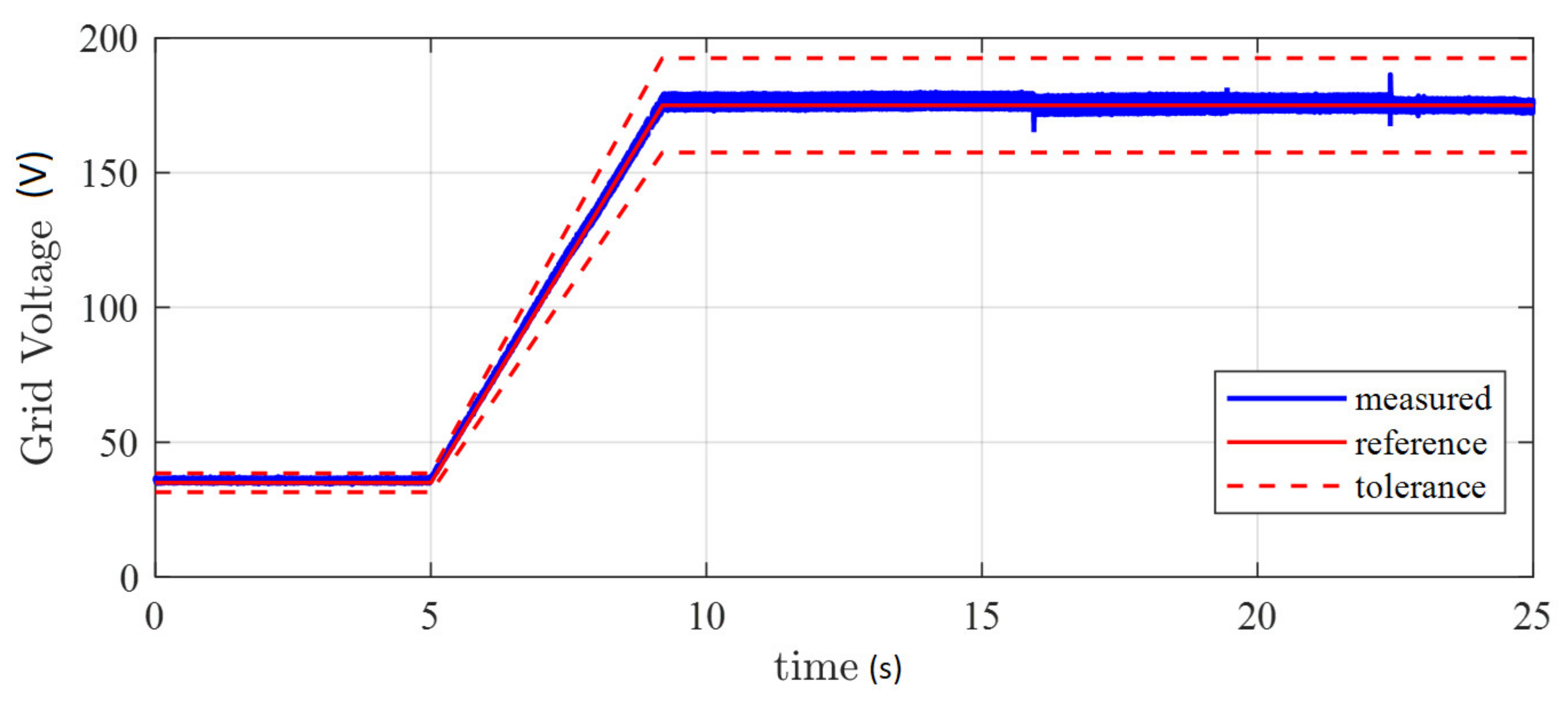
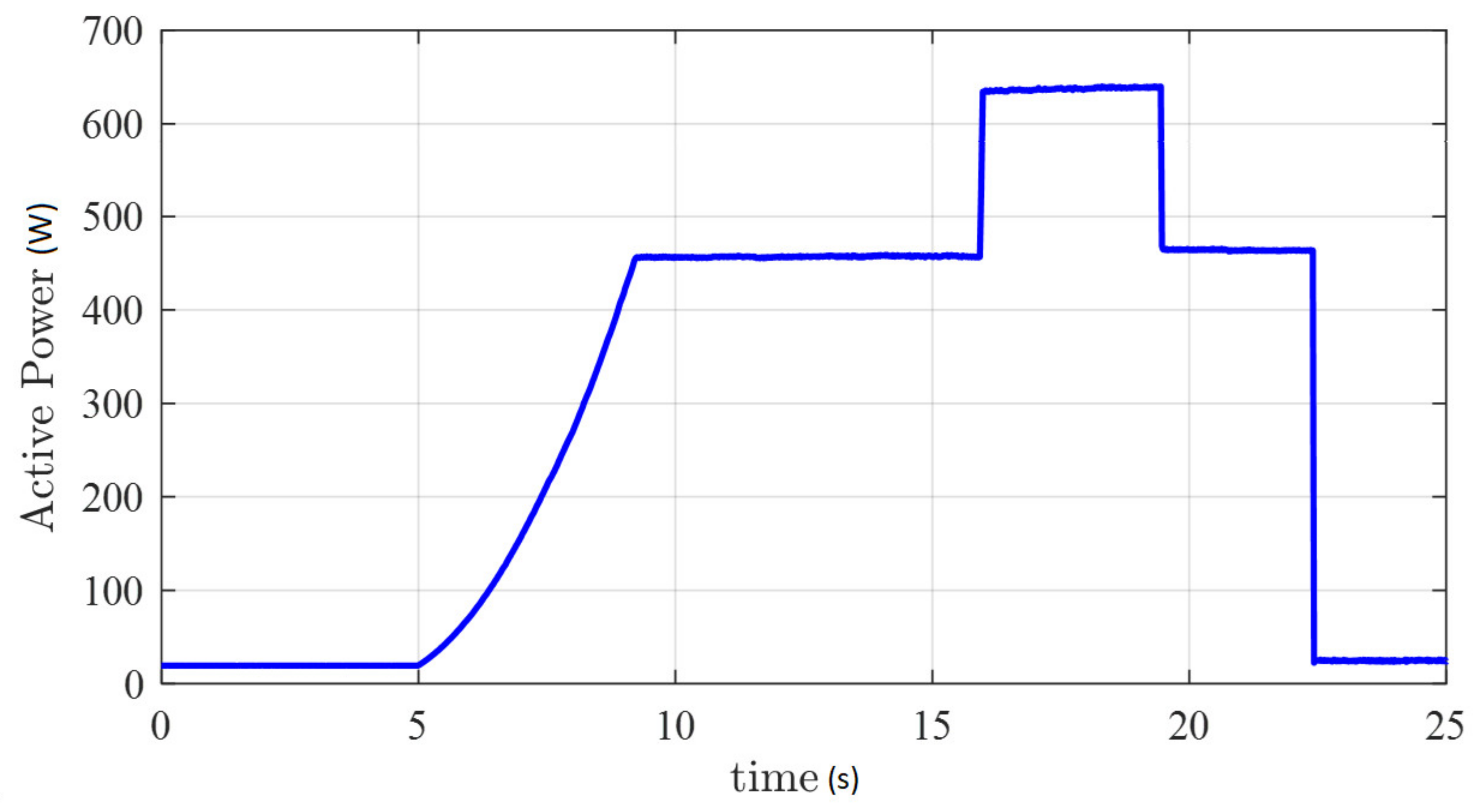
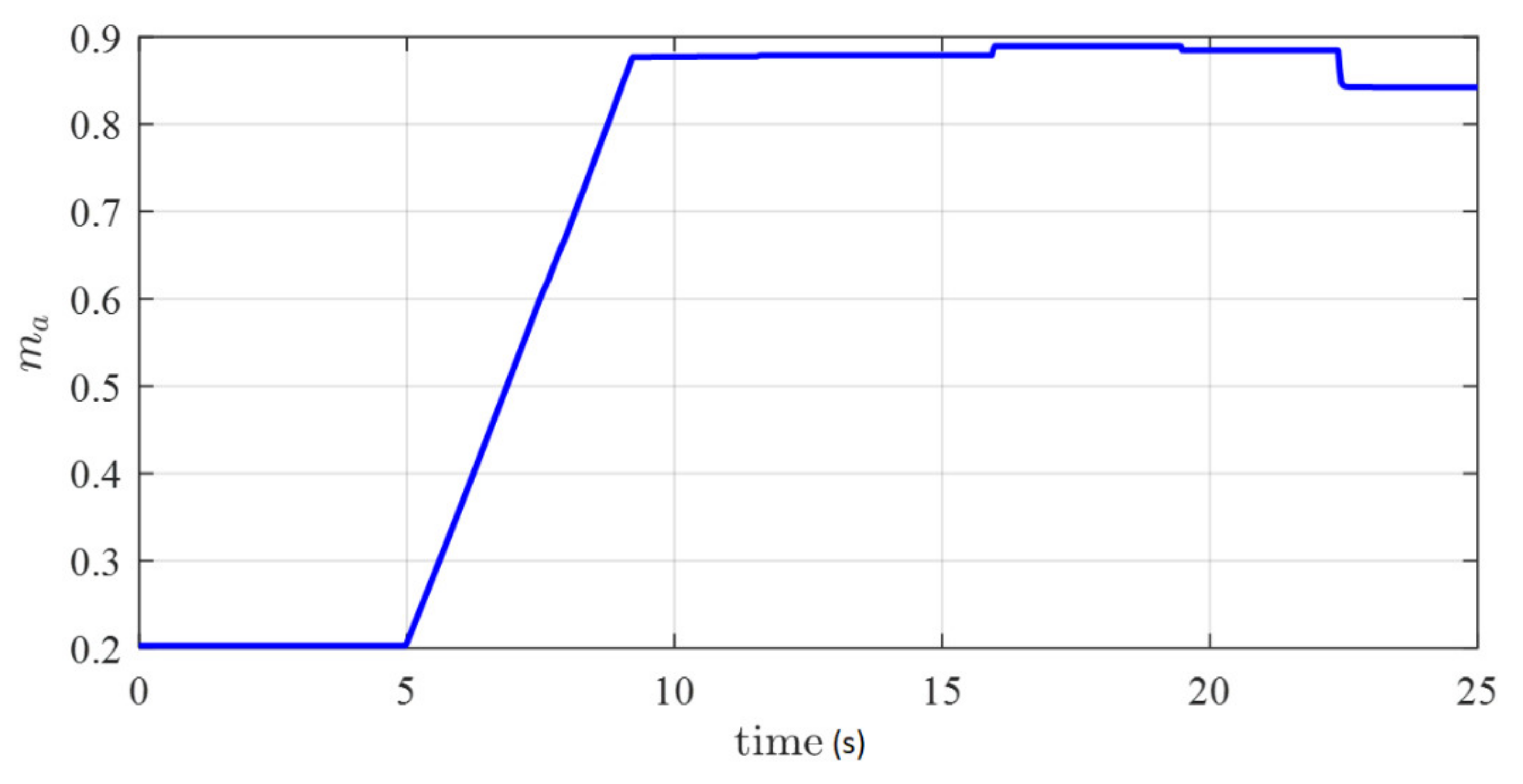
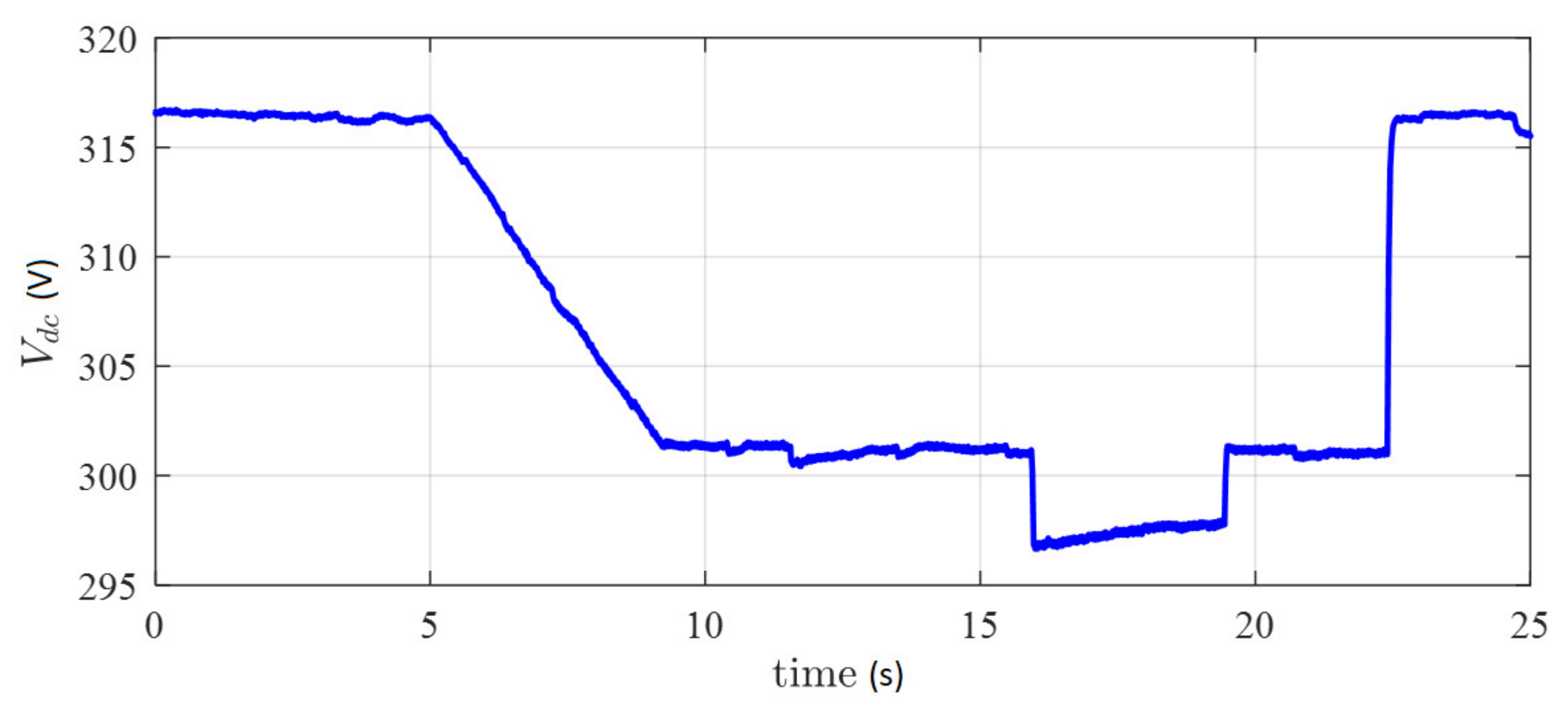
5. Experimental Results

This section aims at describing the HIL test performed to validate the proposed approach. Such a test includes several events in cascade. At first, a ramp increase is provided for the grid voltage, from 35 V to 175 V RMS phase to phase in 4 s, starting at 5 s. This first part allows pointing out the proper operation of voltage control. In this first phase, only Load1 is connected. Secondly, Load2 is connected in parallel with Load1 at 16 s, before being disconnected at 19.5 s. Finally, at 22.3 s, Load1 is also disconnected, leaving the system in a no-load condition.
Figure 10 represents the measured RMS grid voltage; its profile is very satisfactory since it never exceeds the range Vac,ref ± 10%. Instead, Figure 11 shows the active power supplied by the converter.
From Figure 11 one can notice that in the first transient, power increases due to the increase of voltage and the resistive nature of the load. Once that voltage reached its final value, the active power production is equal to 1752/66 = 464 W. Then, at about 16 s, power increases due to the connection of the second load up to ((1/66) + (1/165)) * 1752 = 650 W before reducing progressively up to almost zero (compensating losses in the system). Looking together at Figure 10 and Figure 11, one can notice how the voltage regulation has low sensitivity to power variation, providing a very satisfactory result for the inverter operation. For the sake of completeness, Figure 12 and Figure 13 report the two MPC controller outputs i.e., the modulation index and the modulation frequency.
Finally, Figure 14 highlights the dynamics of the DC link voltage during the experiment. As can be seen from the figure, in correspondence of each load increase, the DC voltage decreases because it is the DC capacitor that initially provides the necessary load power. Then, the DC source current increases providing itself the necessary amount of power for the load, which results in a stabilization of the DC voltage. Please note that no DC voltage controller is implemented here because this would be strictly related to the specific nature of the DC source (e.g., a PV unit should implement a MPPT algorithm, a storage should be equipped with a suitable battery management system and so on).
During this test, the run time of the QP was recorded between 0.78 and 0.91 ms, i.e., shorter than the MPC sampling time (Ts) equal to 1 ms.

6. Conclusions

This paper proposed an innovative control architecture for grid-forming inverter control in islanded MGs. The proposed approach is based on the well-known MPC technique that has been implemented that considers the specific characteristic of the DG unit source on the inverter DC side. In the first part of the paper, the proposed MPC controller has been fully described providing all the necessary information to implement the features of a grid-forming inverter (control goals) accounting for quality ranges of the involved variables (control constraints). After the definition of the proposed MPC controller, the paper focused on the validation of the proposed approach. As well known, the MPC approach usually suffers from implementation issues, due to the fact that it requires the solution of an optimization problem, and this may be too cumbersome from a computational point of view. For this reason, an experimental validation of a proposed control system was performed at the laboratory for electric drives of the University of Niš, Serbia. The experimental validation pointed out the good operation of the proposed controller from both a technical and computational point of view.
On the basis of this important result, the future development of this activity will point to the extension of the proposed MPC approach in a multi-inverter islanded MG, where more than one inverter will have to cope with frequency and voltage regulation. The capabilities of the proposed MPC approach may allow for the elaboration of the design of a communication-less architecture capable of coping with primary regulation in an islanded MG in an effective and reliable way.

Author Contributions

Conceptualization, R.P.; methodology, A.L. and A.B.; software, F.F.; validation, A.L. and F.F.; formal analysis, A.L. and F.F.; investigation, M.P. and A.B.; data curation, A.L.; writing—original draft preparation, A.L.; writing—review and editing, A.L.; visualization, A.B.; supervision, R.P., A.B and M.P.; project administration, M.P. and A.B. All authors have read and agreed to the published version of the manuscript.

Funding

This research received no external funding

Conflicts of Interest

The authors declare no conflict of interest.

Appendix A

The appendix aims to explain how the V/I characterization of the specific powertrain was obtained. The setup is summarized in Figure A1. It is worth reminding that any characterization process is meaningful if the conditions in which the characterization takes place is the same used in the utilization. This means that in the characterization activity DC filter, the diode bridge and autotransformer are the same used and described in Section 3 and Section 4. V/I characteristic was determined by defining 23 different working points (Vdc; Idc) obtained with 23 different values of the resistor Rc in the range (50 Ω–∞) (see dots in Figure 9). Current and voltage measuring devices appear in Figure A1. Then a fitting tool (e.g., Matlab Basic Fitting) allowed to obtain an analytical relationship Idc(Vdc) between DC voltage and current that best fits experimental data. In this work, a 5th order polynomial is used, whose coefficients are listed in Table A1.
Table A1. Polynomial coefficients.
5th4th3th2th1th0
−2.5 × 10⁻⁷ 7.87 × 10⁻⁴−0.471114−2.12 × 1041.27 × 106
Figure A1. Characterization experiment setup.
Energies 13 02270 g0a1

References

  1. Bendato, I.; Bonfiglio, A.; Brignone, M.; Delfino, F.; Pampararo, F.; Procopio, R. Definition and on-field validation of a microgrid energy management system to manage load and renewables uncertainties and system operator requirements. Electr. Power Syst. Res. 2017, 146, 349–361. [Google Scholar] [CrossRef]
  2. Bendato, I.; Bonfiglio, A.; Brignone, M.; Delfino, F.; Pampararo, F.; Procopio, R.; Rossi, M. Design criteria for the optimal sizing of integrated photovoltaic-storage systems. Energy 2018, 149, 505–515. [Google Scholar] [CrossRef]
  3. Bonfiglio, A.; Brignone, M.; Delfino, F.; Invernizzi, M.; Pampararo, F.; Procopio, R. A technique for the optimal control and operation of grid-connected photovoltaic production units. In Proceedings of the 2012 47th International Universities Power Engineering Conference (UPEC), Middlesex, UK, 4–7 September 2012; pp. 1–6. [Google Scholar]
  4. Olivares, D.E.; Mehrizi-Sani, A.; Etemadi, A.H.; Cañizares, C.A.; Iravani, R.; Kazerani, M.; Hajimiragha, A.H.; Gomis-Bellmunt, O.; Saeedifard, M.; Palma-Behnke, R.; et al. Trends in Microgrid Control. IEEE Trans. Smart Grid 2014, 5, 1905–1919. [Google Scholar] [CrossRef]
  5. Shrivastwa, R.; Hably, A.; Melizi, K.; Bacha, S. Understanding Microgrids and Their Future Trends. In Proceedings of the IEEE ICIT 2019, Melbourne, Australia, 13–15 February 2019. [Google Scholar]
  6. Bonfiglio, A.; Barillari, L.; Bendato, I.; Bracco, S.; Brignone, M.; Delfino, F.; Pampararo, F.; Procopio, R.; Robba, M.; Rossi, M. Day ahead microgrid optimization: A comparison among different models. In Proceedings of the OPT-i 2014—1st International Conference on Engineering and Applied Sciences Optimization, Kos, Greece, 4–6 June 2014; pp. 1153–1165. [Google Scholar]
  7. Fornari, F.; Procopio, R.; Bollen, M.H.J. SSC compensation capability of unbalanced voltage sags. IEEE Trans. Power Deliv. 2005, 20, 2030–2037. [Google Scholar] [CrossRef]
  8. Gonzalez-Longatt, F.M.; Bonfiglio, A.; Procopio, R.; Verduci, B. Evaluation of inertial response controllers for full-rated power converter wind turbine (Type 4). In Proceedings of the 2016 IEEE Power and Energy Society General Meeting (PESGM), Boston, MA, USA, 17–21 July 2016; pp. 1–5. [Google Scholar]
  9. Bonfiglio, A.; Invernizzi, M.; Labella, A.; Procopio, R. Design and Implementation of a Variable Synthetic Inertia Controller for Wind Turbine Generators. IEEE Trans. Power Syst. 2019, 34, 754–764. [Google Scholar] [CrossRef]
  10. Rocabert, J.; Luna, A.; Blaabjerg, F.; Rodríguez, P. Control of Power Converters in AC Microgrids. IEEE Trans. Power Electron. 2012, 27, 4734–4749. [Google Scholar] [CrossRef]
  11. Viinamäki, J.; Kuperman, A.; Suntio, T. Grid-Forming-Mode Operation of Boost-Power-Stage Converter in PV-Generator-Interfacing Applications. Energies 2017, 10, 1033. [Google Scholar] [CrossRef] [Green Version]
  12. IEEE Life Senior Member Daley PE DGCP; IEEE Member Houser PE. Assessment of DER Interconnection Installation for Conformance with IEEE Std 1547. In Assessment of DER Interconnection Installation for Conformance with IEEE Std 1547; IEEE: Piscataway, NJ, USA, 2018; pp. 1–18. [Google Scholar]
  13. Hou, X.; Sun, Y.; Yuan, W.; Han, H.; Zhong, C.; Guerrero, J. Conventional P-ω/Q-V Droop Control in Highly Resistive Line of Low-Voltage Converter-Based AC Microgrid. Energies 2016, 9, 943. [Google Scholar] [CrossRef] [Green Version]
  14. Italian Standard C. CEI 0-16—Technical Rules for the Connection of Active Passive Consumers to the HV MV Electrical Networks of Distribution Company; CEI: Milan, Italy, 2008. [Google Scholar]
  15. IEEE. IEEE. IEEE Standard for Interconnection and Interoperability of Distributed Energy Resources with Associated Electric Power Systems Interfaces. In IEEE Std 1547-2018 (Revision of IEEE Std 1547–2003); IEEE: Piscataway, NJ, USA, 2018; pp. 1–138. [Google Scholar] [CrossRef]
  16. Bouzid, A.M.; Guerrero, J.M.; Cheriti, A.; Bouhamida, M.; Sicard, P.; Benghanem, M.J.R.; Reviews, S.E. A survey on control of electric power distributed generation systems for microgrid applications. Renew. Sustain. Energy Rev. 2015, 44, 751–766. [Google Scholar] [CrossRef] [Green Version]
  17. Serban, I.; Ion, C.P.; Systems, E. Microgrid control based on a grid-forming inverter operating as virtual synchronous generator with enhanced dynamic response capability. J. Electr. Power Energy Syst. 2017, 89, 94–105. [Google Scholar] [CrossRef]
  18. Hirase, Y.; Abe, K.; Sugimoto, K.; Sakimoto, K.; Bevrani, H.; Ise, T. A novel control approach for virtual synchronous generators to suppress frequency and voltage fluctuations in microgrids. Appl. Energy 2018, 210, 699–710. [Google Scholar] [CrossRef]
  19. Liu, J.; Miura, Y.; Ise, T. Comparison of Dynamic Characteristics between Virtual Synchronous Generator and Droop Control in Inverter-Based Distributed Generators. IEEE Trans. Power Electron. 2016, 31, 3600–3611. [Google Scholar] [CrossRef]
  20. Arghir, C.; Jouini, T.; Dörfler, F. Grid-forming control for power converters based on matching of synchronous machines. Automatica 2018, 95, 273–282. [Google Scholar] [CrossRef] [Green Version]
  21. Huseinbegovic, S.; Perunicic-Drazenovic, B. A sliding mode based direct power control of three-phase grid-connected multilevel inverter. In Proceedings of the 2012 13th International Conference on Optimization of Electrical and Electronic Equipment (OPTIM), Brasov, Romania, 24–26 May 2012; pp. 790–797. [Google Scholar]
  22. Li, Z.; Zang, C.; Zeng, P.; Yu, H.; Li, S.; Bian, J. Control of a Grid-Forming Inverter Based on Sliding-Mode and Mixed ${H_2}/{H_\infty }$ Control. IEEE Trans. Ind. Electron. 2017, 64, 3862–3872. [Google Scholar] [CrossRef]
  23. Vazquez, S.; Rodriguez, J.; Rivera, M.; Franquelo, L.G.; Norambuena, M. Model Predictive Control for Power Converters and Drives: Advances and Trends. IEEE Trans. Ind. Electron. 2017, 64, 935–947. [Google Scholar] [CrossRef] [Green Version]
  24. Hans, C.A.; Braun, P.; Raisch, J.; Grune, L.; Reincke-Collon, C. Hierarchical Distributed Model Predictive Control of Interconnected Microgrids. IEEE Trans. Sustain. Energy 2018, 10, 407–416. [Google Scholar] [CrossRef] [Green Version]
  25. Zheng, Y.; Li, S.; Tan, R. Distributed Model Predictive Control for On-Connected Microgrid Power Management. IEEE Trans. Control Syst. Technol. 2018, 26, 1028–1039. [Google Scholar] [CrossRef]
  26. Morstyn, T.; Hredzak, B.; Aguilera, R.P.; Agelidis, V.G. Model Predictive Control for Distributed Microgrid Battery Energy Storage Systems. IEEE Trans. Control Syst. Technol. 2018, 26, 1107–1114. [Google Scholar] [CrossRef] [Green Version]
  27. Bonfiglio, A.; Oliveri, A.; Procopio, R.; Delfino, F.; Denegrí, G.B.; Invernizzi, M.; Storace, M. Improving power grids transient stability via Model Predictive Control. In Proceedings of the 2014 Power Systems Computation Conference, Wroclaw, Poland, 18–22 August 2014; pp. 1–7. [Google Scholar]
  28. Babqi, A.J.; Etemadi, A.H. MPC-based microgrid control with supplementary fault current limitation and smooth transition mechanisms. IET Gener. Trans. Distrib. 2017, 11, 2164–2172. [Google Scholar] [CrossRef]
  29. Tavakoli, A.; Negnevitsky, M.; Muttaqi, K.M. A decentralized model predictive control for multiple distributed generators in the islanded mode of operation. In Proceedings of the 2015 IEEE Industry Applications Society Annual Meeting, Addison, TX, USA, 18–22 October 2015; pp. 1–8. [Google Scholar]
  30. Anderson, S.; Hidalgo-Gonzalez, P.; Dobbe, R.; Tomlin, C.J. Distributed Model Predictive Control for Autonomous Droop-Controlled Inverter-Based Microgrids. In Proceedings of the 2019 IEEE 58th Conference on Decision and Control (CDC), Nice, France, 11–13 December 2019; pp. 6242–6248. [Google Scholar]
  31. Dragicevic, T.; Alhasheem, M.; Lu, M.; Blaabjerg, F. Improved model predictive control for high voltage quality in microgrid applications. In Proceedings of the 2017 IEEE Energy Conversion Congress and Exposition (ECCE), Cincinnati, OH, USA, 1–5 October 2017; pp. 4475–4480. [Google Scholar]
  32. Alhasheem, M.; Blaabjerg, F.; Davari, P. Performance Assessment of Grid Forming Converters Using Different Finite Control Set Model Predictive Control (FCS-MPC) Algorithms. Appl. Sci. 2019, 9, 3513. [Google Scholar] [CrossRef] [Green Version]
  33. Allgöwer, F.; Zheng, A. Nonlinear Model Predictive Control; Birkhäuser: Basel, Switzerland, 2012; Volume 26. [Google Scholar]
  34. Bonfiglio, A.; Brignone, M.; Invernizzi, M.; Labella, A.; Mestriner, D.; Procopio, R. A Simplified Microgrid Model for the Validation of Islanded Control Logics. Energies 2017, 10, 1141. [Google Scholar] [CrossRef] [Green Version]
  35. Bonfiglio, A.; Delfino, F.; Labella, A.; Mestriner, D.; Pampararo, F.; Procopio, R.; Guerrero, J.M. Modeling and Experimental Validation of an Islanded No-Inertia Microgrid Site. IEEE Trans. Sustain. Energy 2018, 9, 1812–1821. [Google Scholar] [CrossRef] [Green Version]
  36. Ferreau, H.J.; Kirches, C.; Potschka, A.; Bock, H.G.; Diehl, M. qpOASES: A parametric active-set algorithm for quadratic programming. Math. Programm. Comput. 2014, 6, 327–363. [Google Scholar] [CrossRef]
  37. Ferreau, H.J.; Bock, H.G.; Diehl, M. An online active set strategy to overcome the limitations of explicit MPC. Int. J. Robust Nonlinear Control IFAC-Affil. J. 2008, 18, 816–830. [Google Scholar] [CrossRef]
Figure 1. Elementary scheme for (a) grid forming; (b) grid feeding; (c) grid supporting acting as voltage source; (d) grid supporting acting as current source (adapted from [6]).
Energies 13 02270 g001
Figure 2. Grid-forming base control scheme (adapted from [16]).
Energies 13 02270 g002
Figure 3. Receding horizon technique.
Energies 13 02270 g003
Figure 4. General layout of an inverter-based DG unit.
Energies 13 02270 g004
Figure 5. DG simplified layout used for the MPC controller design.
Energies 13 02270 g005
Figure 6. Generic DG unit control scheme overview.
Energies 13 02270 g006
Figure 7. Experimental electrical layout with evidence of the measuring points and RPC set-up.
Energies 13 02270 g007
Figure 8. Experimental setup details at Niš University: 1—PC with dSpace DS1103; 2—LCL filter; 3—Variable load; 4—DC source; 5—grid inverter; 6—Current sensors; 7—Voltage sensors.
Energies 13 02270 g008
Figure 9. Recorded V/I characteristic of the experimental DC source.
Energies 13 02270 g009
Figure 10. Grid voltage (RMS) time profile.
Energies 13 02270 g010
Figure 11. Active power supplied by the grid-forming inverter.
Energies 13 02270 g011
Figure 12. MPC output—modulation index time profile.
Energies 13 02270 g012
Figure 13. MPC output—angular frequency time profile.
Energies 13 02270 g013
Figure 14. DC voltage across the input DC-side capacitor during the test.
Energies 13 02270 g014
Table 1. Parameters of main passive components.
C1.1 mFRLg11 mΩ
L2.35 mHCf3.3 μF
Li28 mHLg1.3 mH
RLi0.17 Ω
Table 2. MPC controller parameters.
QV3fmin49.5 Hz
Rω10fmax50.5 Hz
RJ5ma,min0.18
N3ma,max1.156
ωn314.159 rad/sAmax4 kVA

