TRIC: A Thermal Resistance and Impedance Calculator for Electronic Packages ^†

Abstract

This paper presents the Thermal Resistance and Impedance Calculator (TRIC) tool devised for the automatic extraction of thermal metrics of package families of electronic components in both static and transient conditions. TRIC relies on a solution algorithm based on a novel projection-based approach, which—unlike previous techniques—allows (i) dealing with parametric detailed thermal models (pDTMs) of package families that exhibit generic non-Manhattan variations of geometries and meshes, and (ii) transforming such pDTMs into compact thermal models that can be solved in short times. Thermal models of several package families are available, and dies with multiple active areas can be handled. It is shown that transient thermal responses of chosen packages can be obtained in a CPU (central processing unit) time much shorter than that required by a widely used software relying on the finite-volume method without sacrificing accuracy.

1. Introduction

The thermal analysis of electronic devices, circuits, and systems has always been an activity of utmost relevance in the semiconductor industry and academia. A thermally aware design can be achieved with the aid of numerical simulations, which are very challenging in terms of CPU time and memory storage, if a high level of accuracy is desired. This has stimulated many research groups to develop tools relying on suitable algorithms to accelerate the solution process (e.g., [1,2,3]).

For the specific case of packaged components, the preferred approach is to build boundary condition independent (BCI) compact thermal models (CTMs) to alleviate the computational burden without perceptible accuracy loss [4,5,6,7]; an interesting review of BCI CTMs for electronic parts is offered in [8].

Standardized procedures have been introduced to allow a fair comparison among packaged components in terms of thermal performances. More specifically, Joint Electron Device Engineering Council (JEDEC) metrics [9] are evaluated and included in the product datasheets. In order to satisfy the request for JEDEC thermal metrics of chosen package families, the authors developed the Thermal Resistance Advanced Calculator (TRAC) tool, the features of which were initially sketched in [10] and then fully described in [11]. TRAC was conceived (i) to allow a straightforward definition of a parametric detailed thermal model (pDTM) of a package with Manhattan geometry/mesh (as well as Manhattan geometry/mesh variations) and (ii) to automatically determine the thermal metrics of the package from the simulated (static) temperature field. TRAC makes use of a model-order reduction (MOR) technique (e.g., [12,13,14,15,16,17,18,19,20,21,22,23]) to transform the pDTM into a CTM, which can be solved in a short time. Various package families were covered, namely, exposed-pad (epad) low-profile (thick) and thin quad flat packages (eLQFPs and eTQFPs, respectively) as well as exposed-pad quad-flat no-leads (eQFN) packages. However, only one heat source (HS) with arbitrary size and position could be activated within the semiconductor die.

TRAC was believed to fulfill the requests of vendors in the semiconductor industry. It has the potential to allow people not necessarily endowed with expertise in the thermal field (such as system engineers, marketing people, etc.) to easily get the thermal metrics of the packages of interest. Additionally, it is suited to free thermal experts from these standard and repetitive tasks, giving them the possibility to focus on crucial thermal issues.

However, as additional package families were considered, soon emerged the need to deal with variations in geometries/meshes much more complex than those manageable by MOR methods like the one implemented in TRAC. For this reason, a new simulation tool referred to as Thermal Resistance and Impedance Calculator (TRIC) [24] has been realized, which enriches the functionalities of TRAC as follows: (i) TRIC relies on a novel advanced projection-based approach that allows deriving CTMs from the pDTMs of package families with Manhattan geometry/mesh and generic non-Manhattan geometry/mesh transformations without efficiency loss; (ii) in addition to the package families available in TRAC, also full-plastic LQFPs (pLQFPs) are included; (iii) the temperature field can also be evaluated under transient conditions; (iv) the pDTMs and the related CTMs of components with multiple HSs can be generated and simulated. It must be remarked that for both pLQFPs and multi-source packages the nature of the geometry/mesh variations is inherently non-Manhattan.

After the contribution [24] was presented, a new TRIC version was released, which also covers eQFN packages with multiple rows of pins (eQFN-mr), as well as PowerSSO packages. Consequently, such a release can handle pDTMs corresponding to a massive amount of package families, which is destined to further increase in the near future.

The aim of this paper is to extend [24] by

• providing an exhaustive picture of the TRIC features;
• reporting and discussing a larger number of results, including those obtained for the newly included package families (eQFN-mr and PowerSSO);
• adding a detailed comparison (only touched upon in [24]) in terms of accuracy and CPU time with the commercial finite-volume (FV) software FloTHERM [25];
• showing a simulated temperature map at a chosen time instant for a multi-source case of practical relevance.

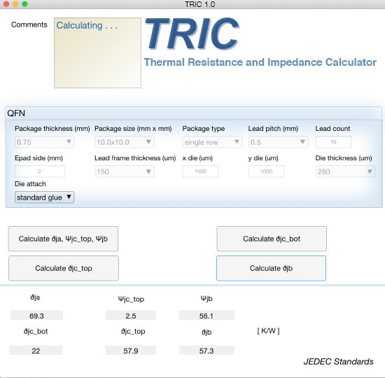
The remainder of the paper is articulated as follows. In Section 2, TRIC is described and the details concerning all the thermally-modeled packages are provided. Section 3 probes into the solution algorithm. The numerical results and the main findings, as well as the comparison with FloTHERM, are shown and discussed in Section 4. Conclusions are then given in Section 5.

2. TRIC Features

TRIC, like the former release TRAC, is suited to automatically extract the JEDEC metrics ϑ_JA, Ψ_JB, Ψ_JCtop, ϑ_JB, ϑ_JCtop, and ϑ_JCbottom in four ambients [9] for each specimen in a package family. The ambients mainly differ in terms of thermal path followed by the heat generated within the HS and emerging from the die; more specifically, the ambient to evaluate ϑ_JCbottom requires a cold plate in intimate contact with the package backside; the plate is located over the top surface when aiming to compute ϑ_JCtop; in the ambient for determining ϑ_JB, a cold ring surrounds the package; no cooling systems are adopted in the ambient common to ϑ_JA, Ψ_JB, and Ψ_JCtop. To this end, a purely conductive pDTM is defined for each family of packages immersed in a specific ambient, within which the boundary conditions (BCs) are calibrated following the JEDEC environment specifications. For instance, for the evaluation of ϑ_JCbottom, an extremely high heat transfer coefficient was applied to the bottom surface to describe the thermal path from the die to the heat sink. The geometry, assumed to be Manhattan (whereas its variation can also be non-Manhattan), is modeled by subdividing the domain into rectangular parallelepipeds (also referred to as cells or, more picturesquely, as bricks) with edges parallel to the x, y, and z axes, for which dimensions, material properties, and heat generation are provided. All data on geometry and properties are stored in a parameter vector p varying in a set P. The pDTM includes information to automatically generate a Cartesian mesh for all specimens belonging to a family of packages in the chosen ambient.

It is worth noting that the pDTMs are created by resorting to reasonable simplifications (coming from the vendor’s experience) that allow a marked reduction in computational burden while negligibly affecting the simulation accuracy. More specifically, in all ambients, the board over which the package is mounted is modeled with a single finely-meshed parallelepiped with a thermal conductivity adjusted to account for the aggregate effect of metal traces and vias, the detailed representation of which would have led to a far too complex problem. In a similar fashion, the pins in the eQFN and eQFN-mr package families, as well as the leads in the pLQFP and PowerSSO families, were thermally represented by a rectangular parallelepiped, the thermal conductivity of which was determined through a weighted averaging procedure.

The thermal metrics can be automatically evaluated through a graphical user interface, in which a chosen specimen in a package family is determined by selecting the corresponding set of parameters. Package size and thickness, pad size, lead count, die size, and thickness are examples of the data that the user can input.

As mentioned in [11], a preliminary convergence analysis of the 3-D mesh discretization of the constructed pDTMs was performed for selected packages; in particular, the calculated thermal metrics were monitored by increasing the degrees of freedom (DoF) until a negligible mesh sensitivity was observed. Then the discretization leading to about 0.1% inaccuracy was chosen to avoid unnecessarily onerous too-fine meshes.

So far, the pDTMs of many package families are available. The list, along with the main geometrical features, is reported below.

• eQFPs, which are surface mount integrated circuit packages with a flat rectangular body, and leads extending from all the four sides. In particular, both the eLQFP and eTQFP variants are available, which differ in terms of body thickness (1.4 and 1 mm, respectively). The square epad structure, which is a standard lead frame wherein the die pad is depressed down to the package bottom face, represents a valuable solution to ease the heat dissipation from die to board. The horizontal size of the body can be 7 × 7, 10 × 10, 14 × 14, 20 × 20, 24 × 24 mm², the total number of leads can be 32, 48, 64, 80, 100, 128, 144, 176, 216 for both variants; several sizes for the epad are available, which span from 3.5 × 3.5 to 9 × 9 mm². Various types of glue for die attach can be selected. The die thickness can amount to 100, 280, 375 (used in the simulations shown in Section 4), and 580 µm (the latter value for the eLQFPs only), while any technologically-reasonable horizontal size can be chosen. It is worth noting that only parameter sets corresponding to real packages fabricated by STMicroelectronics can be selected, whereas all other combinations are obviously not possible; examples are: the 10 × 10 mm² eTQFP with 80 leads can be equipped only with an epad with sizes 3.5 × 3.5, 5.4 × 5.4, 6.2 × 6.2 mm²; many sizes are instead possible for the epad in the 14 × 14 mm² eLQFPs with 100 leads, namely, 3.5 × 3.5, 4.5 × 4.5, 6.0 × 6.0, 7.2 × 7.2, 7.6 × 7.6, 8.5 × 8.5 mm²; 32, 40, and 48 leads are available only for the 7 × 7 mm² eLQFP.
• pLQFPs, where, contrary to the eLQFP counterparts, the mold covers the entire package surface, so that the metal base of the lead frame is not “exposed” and thus not visible from the package bottom. With a few exceptions, all the parameter sets already reported for the eLQFPs are possible.
• eQFN packages, which are lead-less flat molded structures built with a metal lead-frame manufactured by etching, and represent a popular cost-effective and high-performance packaging solution by virtue of the lower inductance than in leaded packages. Several horizontal sizes of the square package body are available, spanning from 2 × 2 to 15 × 15 mm², while the thickness can be equal to 0.55, 0.75, and 0.9 mm (the latter being adopted for the simulations in Section 4). The horizontal sizes of epad and die can be arbitrarily chosen in the ranges allowed by the design rules. Various types of die attach can be selected. Specimens of this family can be equipped with a single row of pins (single-row QFN) or with multiple rows of pins (eQFN-mr), this option being not available in the former TRIC version.
• PowerSSO packages, which are derived from the well-known Small Outline (SO) family and benefit from footprint and height 30%–50% smaller than a conventional dual in-line package. More specifically, epad PowerSSO structures are considered, which are conceived to favor the heat removal without extra cost penalty. Many packages belonging to the PowerSSO family have been included, namely (i) PowerSSO-12, PowerSSO-14, and PowerSSO-16, all sharing a 4.9 × 3.9 × 1.5 mm³ body and equipped with 12 leads (the lead pitch being 0.8 mm), 14 leads (0.65 mm), and 16 leads (0.5 mm), respectively; (ii) PowerSSO-24, PowerSSO-28, and PowerSSO-36, all sharing a 7.5 × 10.3 × 2.3 mm³ body, and equipped with 24 leads (the lead pitch being 0.8 mm), 28 leads (0.65 mm), and 36 leads (0.5 mm), respectively. PowerSSO packages were not covered by the first TRIC release.

Bottom side views of the above-reported packages are shown in Figure 1, while examples of DTMs are depicted in Figure 2. Thermal models of further electronic components can be created with relatively little effort.

Differently from TRAC, in TRIC the evaluation of the temperature field under transient conditions can be enabled for any profile of dissipated power at the HSs. In addition, TRIC allows coping with die layouts integrating circuitries with multiple separate active areas (i.e., HSs), for which the assumption of a uniform power distribution over the whole die surface would have been unacceptably inaccurate. As a result, TRIC can be used with many practical aims. As an example, by emulating the dissipation over the die with only one HS, the thermal impedance can be computed by determining the thermal response to a power step. Moreover, power profiles typically encountered in real applications, like the antilock braking system (ABS) in vehicles, injection, etc., can be taken into account.

3. TRIC Solution Algorithm

The parametric MOR techniques implemented in TRAC are only suited to deal with Manhattan variations of geometry/mesh. A Manhattan transformation is a geometry transformation that converts the x, y, and z coordinates into coordinates X, Y, and Z given by

$$\begin{array}{l}X=f_x\left(x\right)\\ Y=f_y\left(y\right)\\ Z=f_z\left(z\right)\end{array}$$

(1)

with f_x, f_y, and f_z continuous and monotonic functions. Conveniently, contrary to TRAC, TRIC exploits a two-step approach to cope with Manhattan pDTMs associated with non-Manhattan variations of geometry/mesh. This is, for example, the case (i) of pLQFPs, where the relative position of the leads changes by varying the die thickness (Figure 3), and (ii) of multi-source dies, where the relative position of the HSs can be modified (Figure 4).

The functioning principle of TRIC can be described as follows. The DTM of a specimen in a family of packages immersed in a standard environment, automatically extracted by TRIC using the FV method, has the following form:

$$\mathbf{M}\left(p\right)\frac{d\mathit{\vartheta }}{dt}\left(t,p\right)+\mathbf{K}\left(p\right)\mathit{\vartheta }\left(t,p\right)=\mathbf{G}\left(p\right)\mathbf{P}\left(t\right)$$

(2)

in which $\mathit{\vartheta }\left(t,p\right)$ is the N(p) rows vector with the DoF of temperature rise at each time instant t, M(p) is the N(p)-order mass matrix, K(p) is the N(p)-order stiffness matrix, G(p) is the N(p) × M power density rectangular matrix, and P(t) is the M rows vector of source powers.

In the first step, a basis for the projection of (2) is determined by Algorithm 1 exploiting Algorithm 2. In the second step, using this projection basis, a fast solution of (2) is provided for a chosen value of p by Algorithm 3, which again exploits Algorithm 2.

Algorithm 1: Extraction of Projection Basis.
1	form = 1, ... , M do
	for each σ do
	pick a random value p in P
	set ${\widehat{\mathsf{\Theta }}}_m\left(\sigma ,p\right)=0$
	set space Sm(σ): = $\varnothing$
	set ρ: = +∞ (norm of the residual)
	while ρ > ε do
2	solve (2) for ${\mathsf{\Theta }}_m\left(\sigma ,p\right)$ using ${\widehat{\mathsf{\Theta }}}_m\left(\sigma ,p\right)$ as initial guess
3	add $\left(p,{\mathsf{\Theta }}_m\left(\sigma ,p\right)\right)$ to space Sm(σ)
	for Ξ times do
	pick a random value p in P
	apply Algorithm 2
4	compute residual ρ of (2) for ${\widehat{\mathsf{\Theta }}}_m\left(\sigma ,p\right)$
	if ρ > ε do
	break

In Algorithm 1, at line 1, a set of complex frequency values, proper for characterizing the thermal behavior of the family of packages, is chosen following [13]. At line 2, the detailed thermal problem in the complex frequency domain

$$\left[\sigma \mathbf{M}\left(p)+\mathbf{K}\right(p)\right]{\mathsf{\Theta }}_m\left(\sigma ,p\right)={\mathbf{g}}_m,$$

(3)

in which g_m is the m-th column of G and is numerically solved by an iterative solver. A multigrid solver is used, and the number of iterations is reduced by assuming as initial guess the ${\widehat{\mathsf{\Theta }}}_m\left(\sigma ,p\right)$ estimation. At line 3, the solutions ${\mathsf{\Theta }}_m\left(\sigma ,p\right)$ are added to S(σ). At line 4, the residual ρ is determined substituting ${\mathsf{\Theta }}_m\left(\sigma ,p\right)$ with ${\widehat{\mathsf{\Theta }}}_m\left(\sigma ,p\right)$ in (3).

Algorithm 2: Performing Projection.
1	set V: = $\varnothing$
	for each element (q,Θ) of Sm(σ) do
	transform $\mathsf{\Theta }$ into $\widehat{\mathsf{\Theta }}$
	set V: = $[\mathbf{V},\widehat{\mathsf{\Theta }}]$
2	project (3) onto the space spanned by columns of V
3	solve (4) determining ${\widehat{\mathsf{\Theta }}}_m\left(\sigma ,p\right)$ as an approximation of ${\mathsf{\Theta }}_m\left(\sigma ,p\right)$

In Algorithm 2, at line 1, the spatial geometry of the DTM for value p of the parameter vector is expressed as a map of the spatial geometry of the DTM for value q of the parameters vector. This map is thus applied to vector $\mathsf{\Theta }$, getting vector $\widehat{\mathsf{\Theta }}$. At line 2, the projected equations are

$$\left(\sigma \widehat{\mathbf{M}}+\widehat{\mathbf{K}}\right){\widehat{\xi }}_m\left(\sigma \right)={\widehat{\mathbf{g}}}_m$$

(4)

where $\widehat{\mathbf{M}}$ and $\widehat{\mathbf{K}}$ are projected matrices given by $\widehat{\mathbf{M}}={\widehat{\mathbf{V}}}^T\mathbf{M}\left(\mathbf{p}\right)\widehat{\mathbf{V}}$ and $\widehat{\mathbf{K}}={\widehat{\mathbf{V}}}^T\mathbf{K}\left(\mathbf{p}\right)\widehat{\mathbf{V}}$, while ${\widehat{\mathit{\xi }}}_m$ is the DoF column vector and ${\widehat{\mathbf{g}}}_m={\widehat{\mathbf{V}}}^T{\mathbf{g}}_m$. At line 3, vector ${\mathsf{\Theta }}_m\left(\sigma ,p\right)$ is approximated by

$${\widehat{\mathsf{\Theta }}}_m\left(\sigma ,p\right)=\widehat{\mathbf{V}}{\widehat{\mathit{\xi }}}_m\left(\sigma \right)$$

(5)

In Algorithm 3, for a chosen value of p, a space S(p) is determined. Projecting (2) onto such a space, the CTM ensues, the response of which to any power profile is computed for approximating $\mathit{\vartheta }\left(t,p\right)$.

Algorithm 3: Performing Projection

set space S(p):=$\varnothing$

form = 1, ... , M do

for each σ do

apply Algorithm 2

add ${\widehat{\mathsf{\Theta }}}_m\left(\sigma ,p\right)$ to space S(p)

It must be remarked that in commercial numerical codes the complexity for the transient solutions is proportional to (n_x × n_y × n_z)^{α × nt}, where α is in the range 1 ÷ 1.5 (depending on the iterative method adopted); n_x, n_y, and n_z are the numbers of grid points along x, y, and z, and n_t is the number of time instants in which the problem has to be solved. Conveniently, the corresponding complexity in TRIC is proportional to n_t and independent of n_x, n_y, and n_z.

4. Numerical Results

Except for the multi-source analysis (Section 4.4), the intrinsic symmetry of the packages under test allowed meshing and simulating only a quarter of each structure, thus mitigating the computational burden; the missing portions were virtually restored by applying adiabatic BCs (i.e., zero heat flux) over the planes of symmetry.

4.1. Full-Plastic LQFP vs. Epad LQFP

Figure 5 shows the static thermal metrics ϑ_JA and ϑ_JCtop corresponding to eLQFPs and pLQFPs for two horizontal package sizes, namely (a) 10 × 10 and (b) 14 × 14 mm², the epad size being 6 × 6 and 7.2 × 7.2 mm² for cases (a) and (b), respectively. The metrics are determined by TRIC for various sizes of the square die, i.e., 2 × 2, 3 × 3, 4 × 4, 5 × 5, 6 × 6 mm², the latter only for case (b). It can be inferred that the presence of the pad, which eases the heat removal, yields a sizable beneficial impact on ϑ_JA, whereas the closer proximity of the die to the top of the package in pLQFPs prevails over the cooling action of the epad in terms of ϑ_JCtop.

4.2. Thermal Impedances

One of the main features of TRIC not available in TRAC is the possibility to determine the transient thermal responses of a specimen of a package family for any profile of the power sources. In particular, the thermal impedances—often used to characterize the dynamic thermal behavior of components—can be evaluated as the thermal responses (temperature rises normalized to power) to a power step applied at t = 0 to a die modeled with only one HS. Such a capability is witnessed through the analysis of a large set of cases.

Figure 6 shows the junction-to-ambient thermal impedance Z_THJA = ϑ_JA(t) of a 10 × 10 mm² eTQFP equipped with a 6 × 6 mm² epad for four different die sizes. The simulations allow quantifying the favorable influence of a large die, which benefits from a lower power density. Static conditions are reached at about 400 s, regardless of die size. Figure 7 illustrates the Z_THJA of a 10 × 10 mm² pLQFP with a 4 × 4 mm² die for three different pad sizes. All curves coincide for short times (<0.1 s), where the heat emerging from the die has not hit the pad yet. For this case, (i) a complex evolution with an inflection takes place due to the involved package geometry: the heat propagates through the pad, the mold, and then reaches the leads, which are in direct contact with the board, and (ii) the impedances flatten at 1200 s, as induced by the absence of the cooling epad action. Figure 8 reports the Z_THJA of 9 × 9 mm² single-row eQFN packages for three combinations of epad and die sizes. Here the positive influence of a bigger epad (7 × 7 mm² instead of 5.7 × 5.7 mm²) for the same die size is evident; again, the impedances overlap for short times. Similar to the study conducted for the eTQFP family, also for eQFN packages the thermal impedance is reduced and delayed for bigger dies. Figure 9 confirms the cooling impact for medium/long times of a larger package body and/or a larger epad for eQFN-mr packages with two rows of pins. Lastly, the dynamic thermal behavior of a 10.3 × 7.5 mm² PowerSSO-36 with a 4.09 × 3.17 mm² die is determined for four different epad sizes in Figure 10.

4.3. Comparison with FloTHERM

First and foremost, it must be underlined that the user-friendly graphical interface of TRIC allows avoiding the long, painstaking, and prone-to-error geometry/mesh construction process often required by conventional numerical tools, thus markedly lowering the pre-processing effort and time. As far as the accuracy and efficiency of TRIC are concerned, they were estimated by comparison with the widely used commercial software FloTHERM. The tools share the same geometry simplifications and BCs. The favorable matching between the thermal metrics determined by TRAC and the FV software was already shown in [11] for eLQFPs, eTQFPs, and eQFN packages; the slight discrepancy (typically <2%, the maximum value being around 3%) was mainly attributed to the different mesh styles of the simulators. Evidence of the good agreement is also provided in Figure 11, which shows the (static) maps of temperature rise over ambient (T_amb = 20 °C) determined for three eTQFPs with dies dissipating 1 W in the ϑ_JA-related ambient; in particular, (a) corresponds to a 14 × 14 mm² package size with a 9 × 9 mm² epad and a 3 × 3 mm² die; (b) to a 10 × 10 mm² package with a 6 × 6 mm² epad and a 4 × 4 mm² die; (c) to a 10 × 10 mm² package with a 6 × 6 mm² epad and a 2 × 2 mm² die.

The accuracy ensured by TRIC under transient conditions can be inferred from Figure 12, which shows the favorable matching with data computed by FloTHERM for three packages belonging to the eTQFP family. Again, the discrepancy is below 3% within the whole time range. It is worth noting that the CPU time required to obtain an impedance by TRIC for a typical number of 2 × 10⁶ grid points is about 1 min on a workstation with an Intel Xeon E5-2630 v4 @ 2.2 GHz equipped with a 64 GB RAM, whereas more than 15–20 minutes are needed when using FloTHERM. This notable gain in terms of efficiency is expected to take place with respect to most popular simulators based on numerical methods.

4.4. Multi-Source Analysis

Unlike TRAC, TRIC allows also simulating realistic packages that integrate multiple HSs, as evidenced through the following illustrative examples.

First, a 9 × 9 mm² eQFN package is considered, with a 5 × 5 mm² epad and a 4 × 4 mm² die, the latter including four 1 × 1 mm² active areas (i.e., HSs), each dissipating 0.5 W. As sketched in Figure 13, four positions of the HSs are chosen to describe practical layouts. The static temperature rise over ambient was monitored in five critical points, namely, at the die center (ΔT_center) and at the centers of the HSs (ΔT₁, ΔT₂, ΔT₃, ΔT₄). Results corresponding to the four layouts are reported in

Table 1. Temperature rises over ambient (K) computed by TRIC.

	ΔT1	ΔT2	ΔT3	ΔT4	ΔTcenter	ΔTmax
Layout #1	56.31	56.31	56.31	56.31	57.06	57.06
Layout #2	59.56	58.20	58.20	57.05	54.13	59.58
Layout #3	54.89	54.89	54.89	54.89	52.25	55.15
Layout #4	55.77	56.12	56.12	55.77	52.70	56.35

, along with the maximum temperature rise over the whole die (ΔT_max). Again, a fairly good agreement with the temperature maps determined by FloTHERM (not shown here) was obtained, the discrepancy between the maxima being <3%. The data plainly illustrate how the temperature field over the die modifies depending on the specific layout. The main findings are (i) all the HSs share the same temperature in cases #1 and #3 for symmetry reasons; (ii) as expected, in layout #1 ΔT_center = ΔT_max due to the concurrent influence of all the HSs, while (iii) ΔT_max is reached near the die side in layout #2. This simple analysis shows that TRIC can be effectively exploited to identify the most thermally efficient layout. In addition, the information gained on the temperature field over the die is also important to properly place temperature sensors.

4.5. ABS Source Profile

The TRIC capability to cover complex die layouts and transient power profiles is demonstrated by simulating the die temperature dictated by a realistic ABS power profile. The examined package is a 14 × 14 mm² eTQFP with an 8 × 8 mm² epad and a 30 mm² die, the circuitry over which presents eight active areas (HSs), as depicted in Figure 14a. The geometry of the system and the external BCs were adapted to this specific application. Figure 14b illustrates the TRIC interface with the probes (placed at the centers of the HSs) where the temperatures are taken. Figure 14c shows the evolution of the temperature rises over ambient from 0 to 20 s. Figure 14d reports the temperature rise field at the most thermally critical time instant, i.e., 2.5 s.

5. Conclusions

In this paper, a tool denoted as Thermal Resistance and Impedance Calculator (TRIC) has been presented. TRIC allows the automatic extraction of thermal metrics of package families of electronic components under both static and transient conditions. It exploits a solution algorithm based on a novel projection-based approach, which allows dealing with non-Manhattan geometry and mesh variations in the parametric detailed thermal model (pDTM) of a package family. The pDTMs of many relevant package families have been included, and dies with multiple active areas can be handled. An extensive simulation campaign, focused on cases of practical interest, has been performed. A comparison between TRIC and the FV program FloTHERM has been carried out, with the aim of validating the accuracy and assessing the efficiency of the proposed tool; the main findings can be summarized as follows: (i) the discrepancy in terms of thermal metrics calculated by the simulators amounts at most to 3% and is mainly ascribable to the different mesh styles; (ii) thanks to its advanced solution algorithm, TRIC allows obtaining a reduction in CPU time by a factor of 15–20 with respect to FloTHERM when simulating a transient thermal response. Owing to the above reasons, TRIC can be considered particularly helpful for industry specialists who are involved in designing packaged devices and have to cope with thermal flow problems.

References

1. Smy, T.; Walkey, D.; Dew, S.K. A 3D thermal simulation tool for integrated devices-Atar. IEEE Trans. Comput. Aided Des. Integr. Circuits Syst. 2001, 20, 105–115. [Google Scholar] [CrossRef]
2. Huang, W.T.; Ghosh, S.; Sankaranarayanan, K.; Skadron, K.; Stan, M.R. Hotspot: Thermal modeling for CMOS VLSI systems. IEEE Trans. Large Scale Integr. VLSI Syst. 2006, 14, 501–513. [Google Scholar] [CrossRef]
3. Ziabari, A.; Park, J.H.; Ardestani, E.K.; Renau, J.; Kang, S.M.; Shakouri, A. Power blurring: Fast static and transient thermal analysis method for packaged integrated circuits and power devices. IEEE Trans. Large Scale Integr. VLSI Syst. 2014, 22, 2366–2379. [Google Scholar] [CrossRef]
4. Bar-Cohen, A.; Elperin, T.; Eliasi, R. ϑJC characterization of chip packages – justification, limitations, and future. IEEE Trans. Compon. Hybrids Manuf. Technol. 1989, 12, 724–731. [Google Scholar] [CrossRef]
5. Lasance, C.J.M.; Vinke, H.; Rosten, H. Thermal characterization of electronic devices with boundary condition independent compact models. IEEE Trans. Compon. Packag. Manuf. Technol. Part A 1995, 18, 723–731. [Google Scholar] [CrossRef]
6. Pape, H.; Schweitzer, D.; Janssen, J.H.J.; Morelli, A.; Villa, C.M. Thermal transient modeling and experimental validation in the European project PROFIT. IEEE Trans. Compon. Packag. Technol. 2004, 27, 530–538. [Google Scholar] [CrossRef]
7. Sabry, M.N. Flexible profile compact thermal models for practical geometries. J. Electr. Packag. 2007, 129, 256–259. [Google Scholar] [CrossRef]
8. Lasance, C.J.M. Ten years of boundary-condition-independent compact thermal modeling of electronic parts: A review. Heat Transf. Eng. 2008, 29, 149–169. [Google Scholar] [CrossRef]
9. JESD51-12. Guidelines for Reporting and Using Electronic Package Thermal Information; JEDEC: Arlington, VA, USA, May 2005. [Google Scholar]
10. Codecasa, L.; Race, S.; d’Alessandro, V.; Gualandris, D.; Morelli, A.; Villa, C.M. Thermal resistance advanced calculator (TRAC). In Proceedings of the International Workshop on THERMal INvestigation of ICs and Systems (THERMINIC), Stockholm, Sweden, 26–28 September 2018. [Google Scholar]
11. Codecasa, L.; Race, S.; d’Alessandro, V.; Gualandris, D.; Morelli, A.; Villa, C.M. TRAC: A thermal resistance advanced calculator for electronic packages. Energies 2019, 12, 1050. [Google Scholar] [CrossRef] [Green Version]
12. Codecasa, L.; D’Amore, D.; Maffezzoni, P. Modeling the thermal response of semiconductor devices through equivalent electrical networks. IEEE Trans. Circuits Syst. I Fundam. Theory Appl. 2002, 49, 1187–1197. [Google Scholar] [CrossRef]
13. Codecasa, L.; D’Amore, D.; Maffezzoni, P. Compact modeling of electrical devices for electrothermal analysis. IEEE Trans. Circuits Syst. I Fundam. Theory Appl. 2003, 50, 465–476. [Google Scholar] [CrossRef]
14. Codecasa, L.; D’Amore, D.; Maffezzoni, P. Multipoint moment matching reduction from port responses of dynamic thermal networks. IEEE Trans. Compon. Packag. Technol. 2005, 28, 605–614. [Google Scholar] [CrossRef]
15. Codecasa, L.; d’Alessandro, V.; Magnani, A.; Rinaldi, N.; Zampardi, P.J. FAst novel thermal analysis simulation tool for integrated circuits (FANTASTIC). In Proceedings of the International Workshop on THERMal INvestigation of ICs and systems (THERMINIC), London, UK, 24–26 September 2014. [Google Scholar]
16. Codecasa, L.; d’Alessandro, V.; Magnani, A.; Rinaldi, N. Parametric compact thermal models by moment matching for variable geometry. In Proceedings of the International Workshop on THERMal INvestigation of ICs and systems (THERMINIC), London, UK, 24–26 September 2014. [Google Scholar]
17. Magnani, A.; d’Alessandro, V.; Codecasa, L.; Zampardi, P.J.; Moser, B.; Rinaldi, N. Analysis of the influence of layout and technology parameters on the thermal impedance of GaAs HBT/BiFET using a highly-efficient tool. In Proceedings of the IEEE Compound Semiconductor Integrated Circuit Symposium (CSICS), La Jolla, CA, USA, 19–22 October 2014. [Google Scholar]
18. Codecasa, L.; d’Alessandro, V.; Magnani, A.; Rinaldi, N. Matrix reduction tool for creating boundary condition independent dynamic compact thermal models. In Proceedings of the International Workshop on THERMal INvestigation of ICs and Systems (THERMINIC), Paris, France, 30 September–2 October 2015. [Google Scholar]
19. Janssen, J.H.J.; Codecasa, L. Why matrix reduction is better than objective function based optimization in compact thermal model creation. In Proceedings of the International Workshop on THERMal Investigation of ICs and Systems (THERMINIC), Paris, France, 30 September–2 October 2015. [Google Scholar]
20. Codecasa, L.; d’Alessandro, V.; Magnani, A.; Rinaldi, N. Structure preserving approach to parametric dynamic compact thermal models of nonlinear heat conduction. In Proceedings of the International Workshop on THERMal INvestigation of ICs and Systems (THERMINIC), Paris, France, 30 September–2 October 2015. [Google Scholar]
21. Codecasa, L.; d’Alessandro, V.; Magnani, A.; Irace, A. Circuit-based electrothermal simulation of power devices by an ultrafast nonlinear MOS approach. IEEE Trans. Power Electron. 2016, 31, 5906–5916. [Google Scholar] [CrossRef]
22. Rogié, B.; Codecasa, L.; Monier-Vinard, E.; Bissuel, V.; Laraqi, N.; Daniel, O.; D’Amore, D.; Magnani, A.; d’Alessandro, V.; Rinaldi, N. Delphi-like dynamical compact thermal models using model order reduction. In Proceedings of the International Workshop on THERMal INvestigation of ICs and Systems (THERMINIC), Amsterdam, The Netherlands, 27–29 September 2017. (best paper award). [Google Scholar]
23. Codecasa, L.; d’Alessandro, V.; Magnani, A.; Rinaldi, N. Novel approach for the extraction of nonlinear compact thermal models. In Proceedings of the International Workshop on THERMal INvestigation of ICs and systems (THERMINIC), Amsterdam, The Netherlands, 27–29 September 2017. [Google Scholar]
24. Codecasa, L.; De Viti, F.; Race, S.; d’Alessandro, V.; Gualandris, D.; Morelli, A.; Villa, C.M. Thermal Resistance and Impedance Calculator (TRIC). In Proceedings of the International Workshop on THERMal INvestigation of ICs and Systems (THERMINIC), Lecco, Italy, 25–27 September 2019. [Google Scholar]
25. FloTHERM® v12.2. User’s Guide; Mentor Graphics: Wilsonville, OR, USA, 2018. [Google Scholar]
Figure 1. Bottom side views of specimens of the (a) eLQFP, (b) pLQFP, (c) single-row eQFN, and (d) PowerSSO-36 package families.
Energies 13 02252 g001
Figure 2. DTMs of the eLQFP (left), single-row eQFN (center), and PowerSSO-36 (right) families. The black circles represent the temperature probes needed to determine the thermal metrics.
Energies 13 02252 g002
Figure 3. Schematic representation of a non-Manhattan transformation for a pLQFP, where the die (blue rectangle) thickness increases.
Energies 13 02252 g003
Figure 4. Sketch of a non-Manhattan transformation for a multi-source die.
Energies 13 02252 g004
Figure 5. Thermal metrics ϑJA (circles) and ϑJCtop (squares) against die size: comparison between eLQFP (blue) and pLQFP (magenta) for (a) 10 × 10 and (b) 14 × 14 mm2 package size with (a) 6 × 6 mm2 and (b) 7.2 × 7.2 mm2 die sizes.
Energies 13 02252 g005
Figure 6. Thermal impedance ZTHJA vs. time of a 10 × 10 mm2 eTQFP with a 6 × 6 mm2 epad for four different die sizes.
Energies 13 02252 g006
Figure 7. Thermal impedance ZTHJA against time of a 10 × 10 mm2 pLQFP with a 4 × 4 mm2 die for three different pad sizes.
Energies 13 02252 g007
Figure 8. Thermal impedance ZTHJA vs. time of a 9 × 9 mm2 single-row eQFN package for three combinations of epad and die sizes.
Energies 13 02252 g008
Figure 9. Thermal impedance ZTHJA vs. time of various dual-row eQFN-mr packages sharing a die size of 3 × 3 mm2.
Energies 13 02252 g009
Figure 10. Thermal impedance ZTHJA of a 10.3 × 7.5 mm2 PowerSSO-36 L with a 4.09 × 3.17 mm2 die for four different epad sizes.
Energies 13 02252 g010
Figure 11. Temperature rise maps for three eTQFPs dissipating 1 W, as calculated by TRIC (left) and FloTHERM (right): (a) 14 × 14 mm2 package size with a 9 × 9 mm2 epad and a 3 × 3 mm2 die; (b) 10 × 10 mm2 package with a 6 × 6 mm2 epad and a 4 × 4 mm2 die; (c) 10 × 10 mm2 package with a 6 × 6 mm2 epad and a 2 × 2 mm2 die.
Energies 13 02252 g011
Figure 12. (a) Comparison between TRIC and FloTHERM for various eTQFP cases; (b) corresponding percentage error vs. time.
Energies 13 02252 g012
Figure 13. Representation of four layouts corresponding to a four-source die. The temperature-sensing points are located at the center of the die and at the centers of the HSs.
Energies 13 02252 g013
Figure 14. (a) Schematic top-view of the die floorplan; (b) corresponding TRIC interface; (c) evolution of the temperature rises vs. time; (d) temperature rise map at the time instant t = 2.5 s.
Energies 13 02252 g014