Data Driven Optimization of Energy Management in Residential Buildings with Energy Harvesting and Storage

Abstract

This paper presents a battery-aware stochastic control framework for residential energy management systems (EMS) equipped with energy harvesting, that is, photovoltaic panels, and storage capabilities. The model and control rationale takes into account the dynamics of load, the weather, the weather forecast, the utility, and consumer preferences into a unified Markov decision process. The embedded optimization problem is formulated to determine the proportion of energy drawn from the battery and the grid to minimize a cost function capturing a user-defined tradeoff between battery degradation and financial expense by user preferences. Numerical results are based on real-world weather data for Golden, Colorado, and load traces. The results illustrate the ability of the system to limit battery degradation assessed using the Rain flow counting method for lithium ion batteries.

1. Introduction

Due to their intermittent nature, the integration of renewable sources in the energy grid poses several challenges. At the residential level, the energy produced by energy harvesters can be used to satisfy the current load, with the residual energy being fed back into the grid. Intuitively, a wide spread adoption of this model would lead to grid voltage fluctuations, reversals in power flow, frequency variations, and grounding issues [1]. The introduction of batteries to accumulate the residual energy produced by the households for later use can substantially mitigate this issue. However, a mismatch between production and load is often present. For instance, photovoltaic panels have peak generation during the day, whereas load peaks typically occur in the morning and evening. Frameworks aimed solely at the reduction of financial cost incurred by consumers may induce deep charging and discharging cycles of local batteries, which in turn lead to the degradation of battery capacity [2].

The main contribution of this paper is a stochastic control framework for residential buildings equipped with photovoltaic panels and an energy storage unit. The goal of control is to jointly minimize the financial cost of operating appliances to the consumer and the long-term degradation of the battery over time. The key to accomplish this objective is the ability of the controller to predict future load and output of the photovoltaic panels. To this aim, based on real-world data, we build an underlying stochastic model capturing the temporal dynamics of the load and solar irradiance. This latter component of the overall model is particularly convoluted, as the output of the photovoltaic panels depends on a number of factors including geographical location of the building, time of day, and cloud cover. In the framework proposed, the predictor periodically acquires weather forecast and constructs a Markovian model for the temporal dynamics of future solar irradiance.

Based on the models, and using Dynamic Programming [3], the controller evaluates the long-term cost of actions determining the fraction of load satisfied, taking energy from the grid and battery. The former trivially contributes to the financial cost of operations. The definition of a cost capturing the impact of instantaneous actions on longer-term State of Charge (SoC) trajectories of the battery, which determines the capacity degradation rate, is non-trivial. We adopt the approach proposed in Reference [4], where we use Rain Flow to evaluate the degradation rate imposed by charging/discharging trajectories defined by a Markov process and a simple instantaneous cost function to attract the SoC around a specific value.

The rest of the paper is organized as follows. In Section 2 we provide a discussion on related literature. Section 3 describes the system considered in the paper. In Section 3.1, we build the stochastic model capturing the temporal dynamics of the system. Section 3.2 and Section 3.3 introduce control and formulate the optimization problem using Dynamic Programming, respectively. In Section 3.4, we overview the rain flow framework used to evaluate the battery degradation associated with trajectories of the system’s state. Section 4 describes the case-study considered in the paper and presents numerical results illustrating the performance of the proposed framework. Section 5 concludes the paper.

2. Related Work

The current power grid is a unidirectional hierarchical system where energy flows from power plants to consumer loads at the termination points. In this scheme, the power source has no real-time information about consumption. Though this grid has worked well in the past, given today’s increasing concern with climate change, public policy has pushed for a movement away from fossil-fueled based energy, and towards renewables. While the European Union seeks to reconfigure its current grid to achieve 20% increase in energy efficiency, 20% reduction of CO2 emissions, and 20% increase in renewables by 2020, Denmark is seeking renewables as their sole energy source by 2050 [5]. Such a movement towards distributed energy resources necessitates an updated power grid. The “smart" grid requires an integration of components, subsystems and functions under the pervasive control of distributed intelligence [6]. At the residential level, the grid is transitioning from an AC distribution system to household DC-AC hybrid systems as rooftop photovoltaic installations are becoming commonplace.

Central to the success of “smart" grids is the Internet of Things (IoT). As pervasive control has spread in the power system, networked connectivity has also spread into the residential sector in the form of edge devices: appliances, distributed energy resources (DER), and energy storage systems (ESS). IoT has the potential to expand the capabilities of demand side management to the residential sector as home appliances, the energy meter, energy storage, and distributed renewable energy sources become integrated into a larger home energy management system (HEMS) network [7]. Furthermore, Artificial Intelligence (AI) and data-driven methods have recently entered the scene of sustainable energy system design and optimization and have been shown to be promising approaches to achieve technical, economic and social benefits [8].

HEMS is a viable solution in residential demand side management. According to Reference [9], HEMS has to ability to reduce peak demand by 29.6% and operational electricity cost by 23.1%. HEMS leverage IoT connectivity to reduce cost by rescheduling appliances when grid energy is cheaper, provisioning appliance power, interrupting appliance operation, scheduling storage use, and optimizing energy trading [10]. The HEMS, in addition to collecting consumption and monitoring generation, should be able to integrate heterogeneous components including smart and legacy devices [11].

To automate loads and control source generation, HEMS frameworks rely on the construction of a system model over which an optimization metric, subject to uncertainty, is minimized or maximized to drive rule-based control. Although the general HEMS framework remains universal, the methods and models vary depending on the work and the focus of the objective function. Prior art focuses on the scheduling and power optimization of one or more control stage of HEMS. A work may focus on the appliances, the ESS, or the DER but few thoroughly incorporate all devices with proper consideration of all respective stage uncertainties and model unification. HEMS automated load and source control is dependent mainly on two parameters, the prediction of uncertainty with respect to either energy price negotiation and prediction, renewable energy generation prediction, and energy usage prediction. Optimization is then performed to establish load scheduling and power shifting of loads, energy storage scheduling and power optimization, and energy optimization at the renewable generation device [10].

While energy storage management systems are well known in the realm of plug-in electric vehicles, it is a newer concept in HEMS due to the high maintenance cost incurred from battery banks which are subject to degradation over time and energy losses due to DC to AC conversion electronics. In Reference [12], an IoT based HEMS comprised of appliances, renewable energy source (RES), energy storage source (ESS), and a plug-in electric vehicle (PEV) is proposed to satisfy a demand model which takes into consideration the total power consumption of appliance operation, the operation period for the appliance, the length of run-time and appliance priority. While it optimizes the objective as a function of electricity cost, it assumes a one-way flow of energy from the grid to load or the battery to grid respectively. In the Case Study, Reference [12] studies PEV to grid and grid to load battery as two separate configurations constrained by the extent of battery storage capacity. Reference [13] takes a fuzzy logic control approach implementing strategies that optimize power flow between two different energy storage devices in a hybrid fuel cell and battery system. Using hierarchical controllers with a supervisory controller acting as the central hub, the HEMS fulfills appliance energy requests while monitoring the state of battery charge. However, both authors do not address degradation of storage capacity with respect to use.

Hourly power load data was analyzed using Particle Swarm Optimization clustering which required historical data for model training, and linear regression for load prediction in Reference [14]. While Reference [14]’s framework included safety monitoring and appliance schedule, the battery management system also focused on battery capacity without considering how the capacity is a function of use and is susceptible to damage. On the other hand, Reference [15] introduces a DER connected ESS in the form of a photovoltaic tied EV. A charging algorithm based on the predicted photovoltaic output and user preferences is determined by utilizing a mixed integer linear problem that is optimized over the electricity costs constrained by charging level and rate, battery capacity and user convenience. While Reference [16] introduces a PEV management stochastic optimization problem based on the resulting trip time and trip length under varying conditions of electricity price and demand, the authors recognized battery degradation as an alternative optimization parameter for future work. They also assumed a deterministic load profile instead of stochastic load modeling approaches as the focus of their study remained on the state of charge based battery management system. A thorough study [17] on the degradation of the battery lifetime of a plug-in hybrid electric vehicle using a stochastic optimal power management strategy utilized an electrochemistry based model of anode side resistive film formation in lithium ion batteries. Battery management control performed a tradeoff analysis of conflicting objectives to minimize the energy cost and the battery health degradation. Due to the complexity of the model, the set of differential equations had to be reduced and verified experimentally to keep the analysis tractable.

Weather forecasting in ESS tied DER systems is very important as new DC-AC residential hybrid distribution configurations are being entertained to reduce losses that may be incurred through DC-AC power conversions. In these cases, the DC producing DER is fed directly to the ESS. The ESS can then be designed to feed into a DC distributed home system or pass through an inverter to be converted to AC and fed either to the residential load or the back to the grid. Such systems are highly susceptible to the intermittent nature of DER because of their reliance on environmental conditions. Although Reference [15] ignores battery degradation, Reference [15] takes into account the influence of weather on DER in the prediction of estimated photovoltaic output. A weather sensitivity coefficient based on the ratio of the forecast and the actual value for a pre-scheduled period is utilized indirectly in the control. However, the authors do not supplement the weather with additional information from news sources. Reference [14] addresses distributed energy generation under the uncertainty of weather in HEMS for a grid tied rechargeable ESS connected to the DER and main grid. Solar generation was taken into account using regression techniques to predict the indirect power load based on temperature and humidity. In terms of significant environmental factors in the accurate prediction of irradiance for photovoltaics, Reference [18] found that low resolution, ground-based cloud cover data can improve the forecast accuracy of next hour solar global horizontal irradiance (GHI). In this work, the GHI can be determined by means of a lookup table built using nonlinear regression with respect to its corresponding cloud cover value.

More general approaches based on data-driven Model Predictive Control (MPC) have recently gained attention in the context of buildings energy optimization and climate control. For instance the authors of References [19,20] propose a method based on Regression Trees (RTs) and Random Forests (RFs) to build a state-space switched affine dynamical model of a large scale system only using historical data, and thus overcoming complexity of traditional MPC approaches, traditionally based on cumbersome physics-based models. Although the aforementioned studies do not consider energy storage and battery degradation, the proposed framework is very flexible and can be tailored to design and optimize different aspects of HEMSs.

Noting the disparities in approaches to battery SoC sensitive frameworks with an emphasis on degradation, we seek to fill the gap in our proposed HEMS. Furthermore, with the addition of cloud cover and weather forecast complexity we may inform the charge/discharge rate from our DC DER connected ESS. While we do not consider a grid tied ESS, our architecture may be utilized in a DC-AC hybrid home distribution configuration or include power conversion for either a pure AC or DC home distribution. In the case of inverter usage we will assume that conversion losses are lumped into efficiency terms at each stage and that devices are maintained at their ideal operating temperature.

In this work, we seek to consolidate prior art which tend to focus one aspect of HEMS analysis be it the load, ESS, or DER control. Our contributions focus on the design of a unified EMS framework integrating all three IoT components subject to a control policy that minimizes battery degradation and takes into account both historical weather data as well as realtime forecasted data within a time horizon. We build a Markov Decision Process to unify heterogeneous components, and perform dynamic programming and state value iteration constrained by the battery degradation and grid costs to obtain an optimal policy.

3. System Model and Methodology

The residential energy management system while scheduling appliances, must take into account distributed energy resources that the home owner may seek to use as an alternative source of energy or to supplement the energy provided by the utility. The agent must therefore sense current environmental parameters to determine whether energy stored in the battery should be used to supply the residential load during high energy pricing, or whether to charge the battery during high incoming energy from renewables. The components of the distributed energy resource management subsystem of the home energy management system are introduced in Figure 1.

Energy Harvesting Device: The energy harvesting device represents the available microgeneration resource. This power source may be in the form of a small wind farm, fuel cells, small-scale hydroelectric systems, heat pumps, or more commonly rooftop photovoltaic cells. Energy harvesting devices require control especially in cases where the energy generated is in excess of system capabilities either in terms of power storage or supplying the load profile at any given time. Furthermore, the charging rate of the storage device is directly proportional to the amount of energy harvested.

Energy Storage Device: Central to the control system is the home energy storage device. This home energy storage device is comprised of a battery bank that may be comprised of lead acid, lithium ion, or vanadium redox batteries. The lifetime of the battery depends on thermal effects and battery degradation with respect to time. For most battery banks remaining energy capacity, lifetime, and efficiency are directly related to the operating temperature, the depth of discharge, the charging rate, and the number of charge/discharge cycles. To maximize the lifetime of the battery, it becomes necessary to monitor and control the charging rate as it effects the material properties of the electrodes. To increase residential DER popularity, the amount of money saved from switching to renewables must offset the initial installation and maintenance costs of the system as a whole.

Load Profile: The consumer interacts with the system through habitual energy usage. A resident load profile is informed by daily activities. On average, the daily activities of the neighborhood contribute to a local load profile which may be designated as low or high demand at any given time. The system should anticipate changes in load profile, available harvestable energy, and future demand. While in this paper the load takes a more generalized role, Reference [21] allows the profile to be analyzed at a higher behavior specific resolution.

Grid: The utility, or grid, determines the pricing available to the resident at a particular time of day (TOU) or due to specific market demands (dynamic pricing). Depending on the amount of available stored power, charge rate control, and future harvestable power, the home energy management system may choose to draw power from the power grid. The cost of utility supplied power is a function of time with power rates low during off-peak hours and high during peak hours.

3.1. Stochastic Model

3.1.1. Irradiance as a Function of Cloud Cover

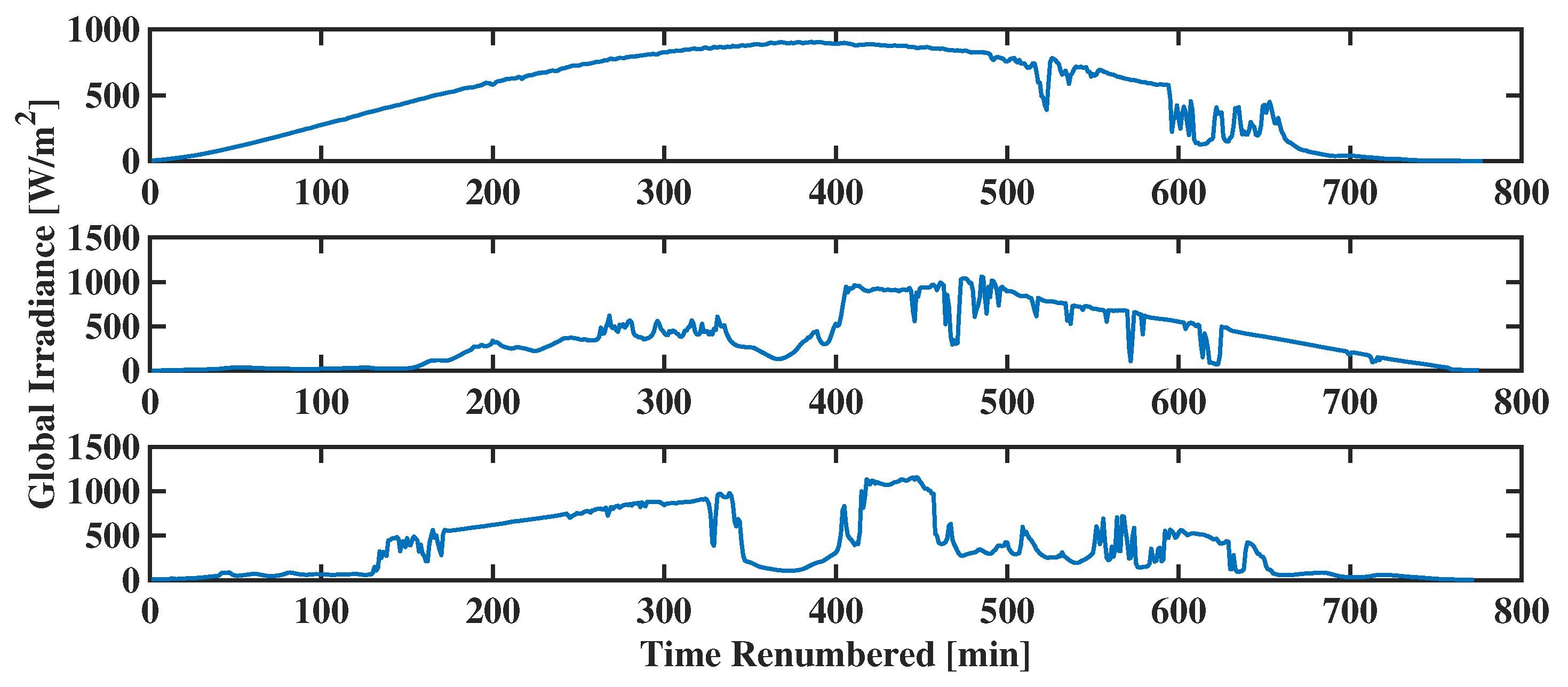
In this section we seek to build a stochastic weather model to find the global irradiance for a specific time of day and a particular cloud cover percentage. We download irradiance datasets from nearby sources or build irradiance records from the resident’s own photovoltaic instrumentation. Ideally, the data should span over a wide variety of cloud cover and weather conditions. We analyze the data for the current month of the year with respect to the same month in previous years in an unsupervised manner. In Reference [22], cloud cover data are used to directly calculate the global irradiance incident on a solar panel based on astronomical and atmospherical constants dependent on the location, time of day, season, and earth’s tilt angle. To simplify and generalize the model, we ignore these parameters and analyze the dataset directly at the ground level. The month chosen for our study is the month of September, and the considered daytime global irradiance dataset is depicted in Figure 2.

The dataset is then divided into daylight hours for each day of the month. Daylight hours result in positive harvestable irradiance measurements, while evening hours result in negative un-harvestable irradiance from below the panel. To further simplify data analysis we note that the variation in irradiance is negligible in adjacent days. Taking this into account we group the individual days of the month into groups of three days which show similar seasonal behavior. Since we would like to compare this model with readily available information we take into account the common meteorological forecasts given for cloud cover. In most weather news outlets, the cloudiness of the day is assessed as “sparse", “partly cloudy", “cloudy," and “overcast." By taking this into account, we bin the cloud cover data into four sets corresponding to cloud cover between 0–25%, 26–50%, 51–75%, and 76–100%. This way we can examine annual irradiance data of three adjacent days in a month for a particular cloud cover state over the course of available records. Therefore, the time series data of global irradiance is divided into varying sequences associated with a particular cloud cover. For example, if the first four datapoints in a time series are associated with a cloud cover of “overcast” followed by two datapoints of “cloudy” and ending with seven datapoints that are “overcast,” this results in two sequences of length four and seven associated with the state “overcast.” Given that we are interested in transitions between irradiance states, single data points in a sequence associated with a cloud cover state are not considered as they do not transition to another state in a time sequence.

While the actual global horizontal irradiance itself follows a Gaussian relationship with some noise, as shown in Figure 3 to capture the variability of cloud cover, we break up the irradiance into hourly time segments and model the system using an inhomogeneous discrete Markov model for the global irradiance as a function of cloud cover and time. The model constructed is inhomogeneous in time to alleviate astronomical and atmospherical considerations in the calculation of irradiance. Without a Markov model, irradiance would have to be deterministically calculated using environmental information that may not be readily available without specific instrumentation. In this model the current state of the irradiance is dependent only on the previous state. We calculate the Markov transition matrix for each hour using the hourly datasets of three day groupings as aforementioned. We bin the global irradiance along all the irradiance data for all hours and sets of three day groupings into a finite number of states across all the datasets for each hour and cloud cover. The data must be binned across all irradiance data for all times of day to ensure that the transition matrices between each hourly time slice contain the same states for matrix dimensions to remain constant. Binning reduces the number of states without significant loss in resolution since the purpose of the weather model is to infer the photovoltaic cell output which depends on the material properties of the semiconductor material beyond a specific threshold voltage.

The Markov transition matrix $g_{ij|C_T,T}$ can be estimated element-wise ${\widehat{g}}_{ij}$ using the global horizontal irradiance data $G_t$ with a finite state space ${\mathcal{S}}_g$ for a given cloud cover $C_T$ for the hour T by calculating the frequency f of transitions from a starting state i to a particular state j over the total number of transitions from state i to all states in the state space.

$${\widehat{g}}_{ij|C,T}=\frac{f_{ij}}{{\displaystyle \sum _{k=0}^{{\mathcal{S}}_g}}{f}_{ik}},$$

(1)

$$\begin{array}{cc}\hfill P(G_{t+1}=g_j|G_t=g_i,C_T,T)& =g_{ij|C_T,T}=\left[\begin{array}{cccc}{\widehat{g}}_{00}& {\widehat{g}}_{01}& \cdots & {\widehat{g}}_{0max({\mathcal{S}}_g)}\\ {\widehat{g}}_{10}& {\widehat{g}}_{11}& \cdots & {\widehat{g}}_{1max({\mathcal{S}}_g)}\\ ⋮& ⋮& \ddots & ⋮\\ {\widehat{g}}_{max({\mathcal{S}}_g)0}& {\widehat{g}}_{max({\mathcal{S}}_g)1}& \cdots & {\widehat{g}}_{max({\mathcal{S}}_g)max({\mathcal{S}}_g)}\\ .\end{array}\right]\end{array}$$

3.1.2. Photovoltaic Power Generation: Energy Harvesting Unit

Since we take into account the local weather forecast and model irradiance as a function of local cloud cover and time of day as a Markov chain, we may calculate the approximate current and power generated for a single photovoltaic panel based on the incident irradiance and manufacturer specifications. Since the photovoltaic cell is comprised of a p-type and n-type semiconductor junction the photovoltaic panel is characterized by its current-voltage or IV relationship as follows:

$$\begin{array}{cc}\hfill i_{out}& \approx i_{sc}(0.001\ast g_t)-i_o[exp(\frac{qv}{nk{T}_k})-1],\hfill \end{array}$$

(2)

$$\begin{array}{cc}\hfill p& =i_{out}\ast v_{mppt},\hfill \end{array}$$

(3)

where $i_{sc}$, $v_{mppt}$, and $i_o$ are current and voltage parameters available in the photovoltaic panel specifications and q, v, n, k, and $T_k$ are physical constants.

The power p output by the photovoltaic panel is assumed to operate at the maximum power point voltage. To ensure maximum power transfer from the solar panel to the energy storage device, we assume maximum power point tracking electronics are employed to maintain a constant voltage $v_{mppt}$. Since the electronics interface with the photovoltaics and home energy storage, some loss in power is expected. Available maximum power point tracking devices are reported to have an efficiency between 94–97%. We can therefore assume that the power input to the battery at any given time can be calculated as

$$p_{in}\approx {\eta }_{mppt}(i_{sc}(0.001\ast g_t)-i_o[exp(\frac{q{v}_{mppt}}{nk{T}_k})-1])·v_{mppt}.$$

(4)

The input power, however, is calculated over a given hour. To get the rate of power charge into the battery, we divide by sixty to calculate an inpute power rate, or energy quanta over a minute since the irradiance for a given cloud cover is subject to changes at a higher resolution than over the hour. We express the value of the harvested quanta H as:

$$\begin{array}{cc}\hfill H_t& =h_i=p_{in}/\mathsf{\Delta }T\hfill \end{array}$$

(5)

$$\begin{array}{cc}\hfill H& =\{H_t=h_i,i,t\in {\mathbb{N}}^{+}\},\hfill \end{array}$$

(6)

where $H_t=h_i$ represents the harvested input energy quanta at discrete time t for a state space ${\mathcal{S}}_{\mathcal{H}}$. $p_{in}$ represents the calculated input power from the energy generating device, and $\mathsf{\Delta }T$ is the period of time we use to scale quanta as a rate. $p_{in}$ is driven by the incident global horizontal irradiance G characterized by the transition matrix $P(G_{t+1}|G_t,C_T,T)$. We can translate G to H as the scaled transition matrix $P(H_{t+1}|H_t,C_T,T)$ allowing us to relate solar irradiance in units of harvested energy quanta available to the battery.

3.1.3. Consumption Load Profile

The consumption load profile, shown in Figure 4 for a given household, is estimated by analyzing individual household load profile data available through the UCI Machine Learning Repository [23].

A sequence of power values are discretized in state space comparable to the state space of the energy harvesting block. We may directly calculate the energy quanta required by the load L by scaling the power to output energy quanta as $p_{load}/\mathsf{\Delta }T$. Since L is dependent on resident power usage susceptible to random variations throughout the day, we express L as a Markov chain and calculate the transition matrix by counting the transitions of a starting state to an individual state averaged over all transitions initiated from the starting state. We repeat the procedure for building a Markov chain from a discretized dataset outlined in Section 3.1.1. We can then express the Markov chain L as $L=\{L_t=l_i,t,i\in {\mathbb{N}}^{+}\}$ for $l_i$ in a discrete state space ${\mathcal{S}}_{\mathcal{L}}$.

3.1.4. Energy Storage Unit

The resident distributed energy resource requires a means of storage to take full advantage of the energy harvested during the daytime. In practice, a battery bank consists of several batteries to increase storage capacity based on energy availability, battery type, and environmental conditions. Several battery types exist on the market such as lead acid, lithium ion, and redox flow for residential battery banks. Differences between the battery types are dependent on the cost, capacity, power ratings, depth of discharge (DoD), round trip efficiency, battery lifetime, and manufacturing [24]. DoD directly affects the battery lifetime and is dependent on the capacity of the battery. If the battery is discharged to maximum capacity the lifetime of the device will decrease over time. Round trip efficiency, the amount of extractable energy given the energy stored, is less than one hundred percent indicating losses incurred from the input power. Furthermore, the amount of charge extracted or inserted to the battery by the load or photovoltaic panel affects the charge/discharge rate of the battery. Battery manufacturers provide warranties covering a certain number of cycles per year given that the battery is operated at optimal conditions and recommended depth of discharge. Since most photovoltaic panels have lifetimes of twenty-five to thirty years, at least one battery bank replacement is expected. To maximize the lifetime of the battery it becomes necessary to control the DoD. The physical properties of the battery also control the extent of charging and discharging as the state of charge varies between low and maximal charge levels [25].

We model the battery bank by assuming that the voltage across all batteries is constant and that the batteries are all of the same type in terms of manufacturing. We assume that the battery banks are in a controlled temperature environment allowing the storage device to operate in ideal conditions exclusive of the ambient temperature outside the home. Furthermore, we model the battery bank as a single battery comprised of discrete quantas of charge to maintain continuity with respect to the unified model in terms of Markov chain characteristics. Each quanta corresponds to a specific charge in the battery and can be described at any time as the superposition of the current battery charge, the proportion of charge drawn from the battery due to the residential load profile, and the input power quanta supplied from the energy harvesting device. Explicitly,

$$Q_{t+1}=Q_t(1-\alpha )+H_t,$$

(7)

where $Q_{t+1}$ represents the energy quanta at the next time trial given that the current value of the energy quanta charge state minus the proportion $\alpha$ of energy quanta drawn from the load and the energy harvest input $H_t$ in unit quanta.

3.1.5. Grid Supply

To take into account modern home energy systems, the residential load profile may draw energy from the battery, the grid, or a combination of the two. The system may choose to take a certain proportion of energy from the storage device and the remaining portion from the grid. The adjusted load seen by the grid energy metering device is the difference between the actual load profile and the proportion of energy drawn from the energy storage device. In other words,

$$L_{gri{d}_t}=L_t-\alpha Q_t,$$

(8)

where $L_{gri{d}_t}$ represents the load from the perspective of the meter at discrete time t, $L_t$ represents the actual resident load, and $\alpha$ represents the proportion of energy $Q_t$ taken from the battery.

While we do not introduce the power electronics associated with inverting the battery power from DC to AC to support the load for simplicity, we remark that the model can be adapted by approximating the inverter with an efficiency term. Indeed in the case study presented, we scale the battery supplied power with an efficiency term.

3.2. Control

Equation (7), while descriptive of the system when connected to the battery, requires that the battery have an adequate amount of existing charge (Q) or input energy harvested (H) in order to meet the load demand (L) at any given time. However, loads that exceed both Q and H may place the residence in outage conditions. The energy management system should be able to choose to take power from the power grid should outage conditions from using the battery alone are encountered. Furthermore, the battery itself has physical limitations with respect to its lifetime and the amount of stresses it can incur upon usage over time. Both of these concerns are addressed in a two-fold control mechanism whereby the residential energy system can be controlled at the power grid to battery level as well as the battery to the energy harvester level.

3.2.1. Load to Battery Connection vs. Load to Grid Connection

In Figure 1, the energy management system may choose to draw a specific amount of power from the battery and the grid in a manner similar to a valve. In other words, the amount of energy taken from the grid and the battery can be tailored to take more power from the grid during off-peak hours to take advantage of pricing and allow the battery to charge. Alternatively, a greater proportion of energy may be drawn from the energy storage unit during ideal battery operating conditions or at times when peak demand causes electricity pricing to fall out of the budget of the resident.

As aforementioned, homes would require interfacing power electronics such as inverters to convert direct current to alternating current, correct for power factor, and feed from the energy harvester to the grid at any given time. Since we model the contributing elements of the home energy system as Markov chains to be used in a Markov decision process for control optimization, the system is subject to the curse of dimensionality. Having a large number of states is undesirable as it requires more processor power which may not be realistic for a simple at home system. We therefore, simplify the process by introducing control in terms of the proportion of energy drawn from the storage unit to the load $\alpha =\{{\alpha }_n,n\in {\mathbb{N}}^{+}\}$, where $0\le {\alpha }_n\le 1$ is a discrete cumulative distribution function characterizing quanta Q. In the case study that follows, the battery quanta are assumed to be equal and uniformly distributed from the minimum capacity to the maximum capacity of the battery. Therefore, the battery charge quanta that can be supplied to the load at any given time is $Q_{sup{p}_t}=Q_t(1-{\alpha }_n)$, where we assume that the battery is drawn at the end of the interval. ${\alpha }_n=0$ represents the condition that no current battery energy is drawn from the battery to supply the load and ${\alpha }_n=1$ represents the condition that all current battery energy is drawn.

It is important to note that the maximum quanta of energy is described by the maximum capacity the battery bank can supply based on its power and charge rating. To tailor the system to meet manufacturer settings it is worth noting that the minimum battery quanta $Q_{min}$ can be set to a value greater than the zero charge level of the battery. Similarly, $Q_{max}$, or the maximum amount of battery charge can be tailored to less that one hundred percent capacity to operate within warranty specifications.

3.2.2. Battery to Harvesting Unit Connection

A second means of control is presented at the battery to the energy harvesting stage of the system which includes the photovoltaic panels and the maximum power point tracking electronics as described in Section 3.1.2. A switch $f_n$ connects the the residential load to the grid or to the battery. The switch $f_n\in \{0,1\}$ where $f_n=0$ is the condition where the battery is disconnected from the harvesting unit and $f_n=1$ is the condition where the battery is connected to the harvesting unit. This second level of charging seeks to mitigate battery damage which if left unattended results inan increase in battery cell internal resistance, reduction in electrode contact, and overall battery capacity fading. The state of charge changes with respect to the configuration of the switches connecting the system components at any given time. For example, if the battery to energy harvesting stage switch is off, the battery is disconnected from the energy harvester which is ideal under conditions of battery saturation or to control the depth of charging in the battery at a given time.

3.2.3. Overall System Dynamics

Following the introduction of two degrees of control, ${\alpha }_n$ and $f_n$, we express the overall system as follows:

$$\begin{array}{cc}\hfill Q_{t+1}& =min(max(Q_t(1-{\alpha }_n)+f_n·H_t,Q_{min}),Q_{max})\hfill \end{array}$$

(9)

$$\begin{array}{cc}\hfill H& =\{H_t=h_i,i,t\in {\mathbb{N}}^{+}\},\mathrm{where}{h}_i\in {\mathcal{S}}_{\mathcal{H}}\hfill \end{array}$$

(10)

$$\begin{array}{cc}\hfill L& =\{L_t=l_j,j,t\in {\mathbb{N}}^{+}\},\mathrm{where}{l}_j\in {\mathcal{S}}_{\mathcal{L}}\hfill \end{array}$$

(11)

$$\begin{array}{cc}\hfill f_n& \in \{0,1\}\hfill \end{array}$$

(12)

$$\begin{array}{cc}\hfill 0& \le {\alpha }_n\le 1,\hfill \end{array}$$

(13)

where $Q_{min}$ and $Q_{max}$ ensure that the charging and discharging of energy quanta remain within the operating parameters of the battery.

3.3. Control Optimization

To optimize the control of proportion of charge taken from the battery ${\alpha }_n$ and the renewable to battery switch $f_n$ we construct a cost function as a tradeoff relationship between the cost of using the power grid and the cost of using battery. The cost of using the power grid can be described by the time of use (TOU) power rate as well as the residential load profile $L_t$ at time t. The cost of using the power grid given the electric power rate $e_{TOU(t)}$ is

$$\begin{array}{cc}\hfill C_g& =e_{TOU(t)}·L_{gri{d}_t}\hfill \end{array}$$

(14)

$$\begin{array}{cc}\hfill C_g& =e_{TOU(t)}·(L_t-{\alpha }_n{Q}_t),\mathrm{where}0\le {\alpha }_n\le 1,\hfill \end{array}$$

(15)

while the cost of taking power from the battery can be approximated as:

$$C_b={(\frac{Q_t}{Q_{max}}-\eta )}^2,\mathrm{where}0<\eta \le 1,$$

(16)

where $Q_{max}$ describes the maximum amount of charge quanta the battery is capable of storing and $\eta$ is a parameter that accounts for charging efficiency. In general, the charging efficiency is a non-linear function of the current SoC and depends on the battery technology and other battery-specific parameters. While several battery energy loss models exist, we take into consideration the generalized approach illustrated in Reference [25] and derived from Reference [26], where the efficiency is approximated as the storage loss of a capacitive device. In the mentioned model, charging efficiency is described as a quadratic function of the SoC and has a maximum at the 50% of the SoC. Accordingly, we set $\eta =0.5$, indicating that the battery charges most efficiently when $Q_t=0.5·Q_{max}$. $Q_t$ close to $Q_{max}$ results in less charge efficiency as the battery has already reached a state of saturation. For values of $Q_t$ close to zero the battery has little to no charge stored. The energy it takes to overcome the charging inertia of an empty battery is high so the state of charge efficiency is low. To construct a tradeoff between the physical costs of battery usage $C_b$ and grid usage $C_g$ requires that both values are normalized in a manner that can be superimposed into one defining cost function. This function may then be used in the dynamic programming value iteration method for Markov decision processes. We observe that the value of $C_b$ remains within $[0,1]$ whereas the value of $C_g$ depends on the current TOU grid pricing. This observation, if unattended would result in a poor evaluation of the ideal Markov policy output of the value iteration function as the units and cost scales are mismatched. To alleviate this situation, we normalize $C_g$ by the maximum power $L_{max}$ that the resident is capable of drawing when all appliances in the home are on. We rewrite the cost of the grid as:

$$C_g=\frac{e_{TOU(t)}·(L_t-{\alpha }_n{Q}_t)}{e_{TOU(t)}·L_{max}}=\frac{L_t-{\alpha }_n{Q}_t}{L_{max}}.$$

(17)

We can now formulate the overall system cost function using the tradeoff factor $\lambda$ associated with the action parameters ${\alpha }_n$ and $f_n$ as:

$$\sum C=\lambda ·C_g+(1-\lambda )·C_b$$

(18)

and thereby apply the value function iteration for Markov decision processes to arrive at an optimal policy or sequence of ${\alpha }_n,f_n$ actions.

Value Function Iteration

In this section we introduce the construction of the value function iteration parameters using the Markov system quantities defined as well as the introduction of hourly weather forecast in terms of cloud cover for the consumer residence location. We define the value function for a Markov decision process using the Bellman equations. In other words, given the system state space S, the model $P(s^{\prime }|s,a)$, the actions $A(s)$, the state action space $\mathcal{S}\times \mathcal{A}$, the cost $C(s,a)$, and the discount factor $0\le \gamma \le 1$, we may derive an optimal policy $\mathsf{\Pi }(s)\to a$ or a sequence of state-actions for the system for a time horizon of interest. The Bellman equations describing the generalized process are [3]:

$$\begin{array}{cc}\hfill V(s)& =\underset{a}{min}(C(s,a)+\gamma \sum _{s^{\prime }}P(s^{\prime }|s,a)V(s^{\prime }))\hfill \end{array}$$

(19)

$$\begin{array}{cc}\hfill Q(s,a)& =C(s,a)+\gamma \sum _{s^{\prime }}P(s^{\prime }|s,a)\underset{a}{min}Q(s^{\prime },a^{\prime }).\hfill \end{array}$$

(20)

The second Bellman equation is written in terms of what is known as a Q-state or state-action pair for a given time. Note that in the value function method the system recursively calculates the updated value using the previous value. In the Q-state packaging of the Bellman value iteration, the cost for all state action pairs for a given time step are calculated. The state-action pair that results in the minimum cost is thereby used in the iteration for the next state calculation. In terms of the established system parameters we may describe the residential energy Markov decision process in terms of the state $s=(H_t=h_i,Q_t=q_j,L_t=l_k)$ with state space ${\mathcal{S}}_{\mathcal{H}}\times {\mathcal{S}}_{\mathcal{Q}}\times {\mathcal{S}}_{\mathcal{L}}$, model $P(H_{t+1},Q_{t+1},L_{t+1}|H_t,Q_t,L_t,{\alpha }_n,f_n)$, action $({\alpha }_n,f_n)$, state-action $s,a=(H_t=h_i,Q_t=q_j,L_t=l_k),(f_n,{\alpha }_n)$ with state-action space ${\mathcal{S}}_{\mathcal{H}}\times {\mathcal{S}}_{\mathcal{Q}}\times {\mathcal{S}}_{\mathcal{L}}\times {\mathcal{S}}_{{\alpha }_n}\times {\mathcal{S}}_{f_n}$, cost $C(s,a)=\lambda ·C_g((H_t,Q_t,L_t),({\alpha }_n,f_n))+(1-\lambda )·C_b((H_t,Q_t,L_t),({\alpha }_n,f_n))$, and the discount factor $0\le \gamma \le 1$. A visual representation of this value iteration is presented in Figure 5. We may derive an optimal policy $\mathsf{\Pi }(s)\to a$ or a sequence of state-actions for the system for a time horizon of interest.

3.4. Battery Degradation

During each battery charge and discharge cycle microscopic structural damage occurs within the material. For narrow-band Gaussian processes, the cycles are well defined, however for general stress information cycle counting methods are useful. In time domain, fatigue analysis uses the information provided by local maxima and local minima in stress data. This allows the stress ranges to be identified and grouped using cycle counting methods. ASTM E 1049-85 establishes the rain flow counting method as a standard suitable for fatigue damage [27].

3.4.1. Rain Flow Counting Method

Using the Rain flow method as outlined in [28], the cyclic stress can be found by

$${\sigma }_{ampl}=\frac{{\sigma }_{max}-{\sigma }_{min}}{2},$$

(21)

where ${\sigma }_{max}$ and ${\sigma }_{min}$ correspond to a maxima or minima in stress data and $ampl$ corresponds to a particular path between extrema. Following the calculation of stress ranges for each individual path defining a half cycle, the paths can be grouped according to the range of $\sigma$ and the number of cycles $n_g$ for a each group g which is simply the sum of the half cycles associated with each group of similar cycle. The damage for any particular group g of paths of equal stress range $\sigma$ can be assessed by examining the material’s characteristic Wöhler/S-N curve of cyclic stress. This curve is a bi-logarithmic graph which represents how well a material can withstand stress cycles. In other words it is characterized by

$$log({\sigma }_{ampl})=log({\sigma }_{fail})-mlog(N),$$

(22)

where ${\sigma }_{fail}$ is the stress at static failure (maximum yield strength) and N is the number of cycles. The maximum number of cycles can be calculated by manipulating Equation (22), to:

$$N_{max}={(\frac{{\sigma }_{fail}}{{\sigma }_{ampl}})}^{\frac{1}{m}},$$

(23)

where m represents the slope of the ${\sigma }_{ampl}$ vs N curve. The S-N, or Wöhler curves are readily available for construction materials such as steel, iron, and aluminum. Lithium ion Wöhler curves are difficult to find and must be estimated based on other fatigue parameters. In this work we use the methods introduced in [29] to approximate the S-N parameters for fatigue life calculation of the battery given the battery charge/discharge history. The fatigue life calculation gauges the effectiveness of control in extending the battery life while minimizing the cost of taking power from the grid.

3.4.2. Cumulative Material Damage

The Palmgren-Miner [30] cumulative fatigue damage D is approximated as

$$D=A_1{(\frac{{\sigma }_{ampl}}{{\sigma }_{fail}})}^{\frac{1}{m}}·Cycle,$$

(24)

where $A_1$ is the capacity loss percentage factor and ${\sigma }_{fail}$, and m are experimentally derived values. In our analysis we use the values fitted in the study presented in [29], which we report in

Table 1. Approximate Damage Constants.

$A_1$ [%/cycle]	0.04519
m	0.4926
${\sigma }_{fail}$ [MPa]	8

for completeness.

4. Results

In this section we provide a case study demonstrating the optimization control of a residence in Golden, CO from 1–3 September 2016. Golden, CO was chosen as a location due to its variety and complexity of weather patterns and cloud cover. The month of September was chosen due to the daytime hours which roughly equal the amount of dark hours during the day. The models were built using historical weather and irradiance datasets available through the National Renewable Energy Laboratory from 2005–2015 after discretization and preprocessing. The consumption load profile for a given household was estimated by analyzing individual household load profile data available through the University of California, Irvine Machine Learning Repository [23]. Forecast information was web-scraped from weather channel information for up to nine hours beyond the current time.

The grid costs were based on the hourly rate advertised by the local utility which varied depending on the time of use and peak demand hours. However, in the end the cost was normalized and dependent proportionally on the difference of the present load and the drawn battery power with respect to the grid at a given time. Battery costs were determined using the operational physical equations presented in Section 3.4. The battery parameters used for this study are for lithium ion presented in Reference [29]. The value function was run over the forecast data starting four hours from the present time. Following the evaluation of the cumulative sum of the costs, the action associated with the minimum cost at the present time for the present cloud cover information was chosen. Actions were chosen every 15 min taking advantage of forecast data. The simulation then ran for the present hour. Upon the start of the next hour, the value function was evaluated starting four hours into the future using the forecasted data until sunset when the system was no longer receiving solar radiation.

Simulations for the system Markov Decision Process were performed for $0\le \lambda \le 1$ in increments of $\lambda =0.05$. For one thousand sample functions of load and irradiance given cloud cover and hour, the battery charge and discharge profiles based on varying cost functions were assessed in terms of aging. Simulation results show the predicted irradiance based on the cloud cover from the forecasted data as well as the Markov model. The irradiance due to the binning algorithm to reduce states result in quantized outcomes that are apparent in the artifacts present in the simulated irradiance profile H in Figure 6. 3 September is analyzed and presented due to its variability with respect to cloud cover. The load profile model has been isolated to daylight hours associated with the averaged dataset and is labeled as L. Recall that the total cost in general was expressed as $C(s,a)=\lambda C_g(s,a)+(1-\lambda )C_b(s)$ where the cost was a function of both the current system state generalized as s and the action generalized as a. Recall $C_g$ an $C_b$ are the grid and battery costs respectively. Results support improved system dynamics with energy management system implementation. We observe in Figure 6 that the charge discharge profile of Q is very much dependent on the cost parameter $\lambda$. In other words, when $\lambda =0$, the system minimizes battery damage maintaining the ideal operating point of fifty percent of the total charge capacity. In this case, the system prioritizes minimization of battery aging exclusively. Conversely, when $\lambda =1$, the system minimizes grid cost exclusively and draws battery quanta from the energy storage unit thereby resulting in greater deviations from the ideal operating point and depth of discharge. In the case where $\lambda =0.5$ both the grid cost and the battery aging cost are weighted equally. From varying the value of $\lambda$, it is clear that when optimization favors the battery the fluctuations in charge discharge cycles are flatter ($\lambda =0$). When $\lambda$ is tuned with some favoring towards the grid, $0.5<\lambda \le 1$, the fluctuations from the ideal operating point increase as the battery is charged and discharged more readily as illustrated in Figure 6.

Figure 7 presents the averaged battery degradation or damage calculated after the charge discharge profiles of Q for each lambda value $0\le \lambda \le 1$ of one thousand sample functions of irradiance H and load L data are generated. The turning points of the charge profiles are then calculated. Upon rainflow analysis using the physical parameters from [29], we observe that $\lambda$ as defined in the optimization cost function is directly proportional to the battery aging degradation. Averaged results over one thousand samples are presented in Figure 7. In other words, as the cost parameter $\lambda$ increases, the control favors usage of the battery over usage of the grid resulting in greater battery degradation as illustrated in Figure 8.

5. Conclusions and Discussion

In this work, we presented a stochastic framework based on Markov decision processes for the optimization of energy management in residential building settings with energy harvesting and storage. The proposed approach is based on real-world data that include weather forecasting and typical daily hour consumption profiles. The considered optimization problem aims at determining the proportion of energy drawn from the battery and the grid to minimize a cost function capturing a user-defined tradeoff between battery degradation and financial expense by user preferences. The novelty of the proposed methodology lays in the explicit inclusion of battery dynamics (i.e., charging/discharging profile) as key aspect of the system design and optimization with the objective of extending the battery life span. Numerical results, produced for a specific case study, reveal an interesting tradeoff between battery degradation mitigation and utility side costs reduction. Importantly, including battery aging phenomena in the optimization rationale yields, in general, a local increment of financial cost for the user given that battery preservation encourages to request power from the grid. Nevertheless, financial cost increment is compensated by a prolonged battery life.

In our analysis we took into consideration a single family home as a prosumer. The proposed method can be extended at a larger neighborhood scale. This would require additional game theoretic approaches as community-level energy harvesting stations would require individual residents to make requests depending on individual consumption needs. In this case, the utility would have to work at the community level and additional constraints would have to be considered in the optimization problem. The scalability of such a system to a larger group, community, neighborhood, county, city level would require further developments and terms in the model to take into consideration of broader system level behavior which may be influenced by additional patterns such as traffic, events, and other factors that may influence load demand in any given location. This may be done so by adding to the graphical model and taking each household Markov chain as an aggregate cluster or state within larger hierarchical Markov chains but doing so would increase the state space of the framework. Additional methods utilizing deep learning to build larger systems that then can be used in a reinforcement learning paradigm specific to each level may present a slightly generalized approach. The challenge to scaling up the framework would be to prevent the model from turning intractable state-wise, keep the framework versatile to impactful sparse information and events, and define an accurate cost function to define the control with which the agent would make decisions on.

Moreover, our approach could aid in the efficiency and control of data centers which are highly dependent on server load demands and require elaborate cooling systems. While some progress has been made in load prediction using feed-forward neural networks at Google/DeepMind [31] resulting in a 40% improvement in efficiency, we believe additional work using alternative hierarchical and probabilistic frameworks such as the one presented in this work may result in further energy savings and development of AI approaches to the energy domain [32].