Design of an Observer-Based Architecture and Non-Linear Control Algorithm for Cogging Torque Reduction in Synchronous Motors

Abstract

The problem of cogging torque is due to a magnetic behavior, intrinsic to synchronous machines and due to the presence of permanent magnets themselves. Cogging torque is a significant problem when the servo drive is used for applications where high precision in terms of position control is required. In this paper we present a method of cogging torque reduction by means of a control technique based on mathematical modeling of the cogging phenomenon itself in order to exploit this knowledge directly in the controller design. The mathematical model is inserted in the dynamic model of the synchronous machine in order to exploit the feedback linearization, providing an expression of the control law in which the contribution of the deterministic knowledge of the phenomenon is directly present. The cogging phenomenon physically depends on the angular position of the rotor, as well as the deterministic model we use to define the control vector. This makes it interesting and innovative to determine whether the control algorithm can be inserted within a sensor-less architecture, where rotor position and angular velocity measurements are not available. For this purpose, we present the use of an extended Kalman filter (EKF) in the continuous-time domain, discussing the advantages of an observer design based on a dynamic motor model in three-phase and direct-square axes. Results are presented through very accurate simulation for a trajectory-tracking problem, completing with variational analysis in terms of variation of initial conditions between EKF and motor dynamics, and in terms of parametric variation to verify the robustness of the proposed algorithm. Moreover, a computational analysis based on Simulink Profiler is proposed, which provides some indication for possible implementation on an embedded platform.

1. Introduction

In the following section we introduce the problem of cogging torque suppression in synchronous/brushless power drive systems when the goal is to use also a sensor-less architecture, in which there is no availability of an encoder/resolver or any other kind of measurements of rotor axis positioning/speed.

We want to highlight that the novelty of our work in the usage of a sensor-less power drive system architecture in the context of cogging torque reduction for applications where the precision of rotor axis positioning control is an important issue in order to have good trajectory tracking. An example of these applications is robotic manipulation for “pick and place” operations.

In this work we present the combination of the feedback linearization non-linear control technique and the extended Kalman filter (EKF) designed considering a continuous time domain model, exploiting the three-phase axis representation of the synchronous motor dynamic. In this work we introduce also the technical motivation to prefer the usage of an augmented size of the estimated state vector dynamic of the observer system, referred to the three-phase motor dynamic model, instead of the direct-quadrature axis as often used in literature.

As explained in following sections, the usage of a higher dynamic cardinality of the reference model for the observer design has the advantage of being able to avoid possible algebraic loops related with the continuous time domain EKF application, although it requires a little increase of computational complexity.

We want to remark that in our work the novelty is in the cogging torque reduction through a non-linear feedback linearization (FLC) technique that takes in care also the usage of a continuous time domain EKF in the design of a sensor-less position trajectory control architecture. Most of the works in literature exploit observer-based control architectures in applications for speed control of the electric machine which do not require a very high precision in rotor axis positioning (as for example in electric vehicle power trains or in unmanned ground vehicles). Highlighting the contribute of our work, other articles which exploit a sensor-less architecture for the rotor axis positioning control of an electric motor does not present an application specific for the cogging torque reduction. In general, there are very few works that take into consideration the intrinsic cogging Torque physical phenomenon. In the following we briefly explain the cogging torque phenomenon and why it is an issue in rotor axis positioning for synchronous power drive systems. We explain also why is challenging from a control algorithm point of view the usage of a sensor-less architecture in the context of the reduction of such a phenomenon. The cogging phenomenon is an intrinsic physical behavior related with the presence of the permanent magnet arranged in the rotor iron. In particular, the magnets are arranged along the rotor surface in the surface permanent magnet (SPM) internal architecture otherwise the magnets are embedded in rotor iron itself in the case of Interior Permanent Magnet (IPM) internal architecture. The cogging phenomenon occurs both in SPM or IPM internal architecture of the electric machine and the final effect on the rotor axis positioning is the same, anyway in the following reference is made to an SPM rotor structure. The cogging phenomenon is due to the magnetic field produced by the permanent magnets arranged on the rotor surface which interact with the teeth of the stator caves. The magnetic flux causes a couple of magnetic forces which can be represented as applied in the center of the magnets in which the magnetic flux is enclosed and tangent to the flux itself. This couple of magnetic forces has the tendency to align the center of the magnets with the center of the closest tooth of the caves, in order to reach the minimum energy configuration. Intuitively, during the rotation of the rotor axis there are some configurations in which, with respect to a certain couple magnet-tooth, the force caused by the magnetic interaction can be under attractive force or repulsive force depending of the mutual rotor positioning between rotor and stator. The sum of all the couple of forces related with each magnet-tooth couple is in fact the cogging torque that can be considered with zero mean value by the fact that the internal geometry of an electric machine has cylindrical symmetric properties. Under this consideration, it is possible to affirm that the cogging torque can be interpreted as an additional torque disturbance signal respect the electromagnetic torque, dependent to rotor axis position with intensity related to the internal structure of the motor itself (number of pole pairs, teeth geometry, air-gap thickness). Cogging torque is an intrinsic issue related with any kind of synchronous/brushless electric motor as reported in the theory of permanent magnets machine [1,2] and more modern revision of the design procedures for different structure and geometry [3,4]. In this work we consider a classic cylindric geometry with SPM internal structure but our result is not limited to the SPM geometry and can be easily extended to IPM or any kind of synchronous machine changing the dynamic model in order to take care about the differences (as anisotropic effect, saliency of the magnets, etc.).

After this introduction, the paper is organized as follows: Section 2 deals with cogging torque modeling and analysis of sensorless power drive architecture, Section 3 reviews state-of-art state observer and cogging torque reduction techniques, Section 4 presents the design of the proposed control system, Section 5 shows simulation results. Conclusions and future work are discussed in Section 6.

2. Cogging Torque Modeling and Sensorless Power Drive System

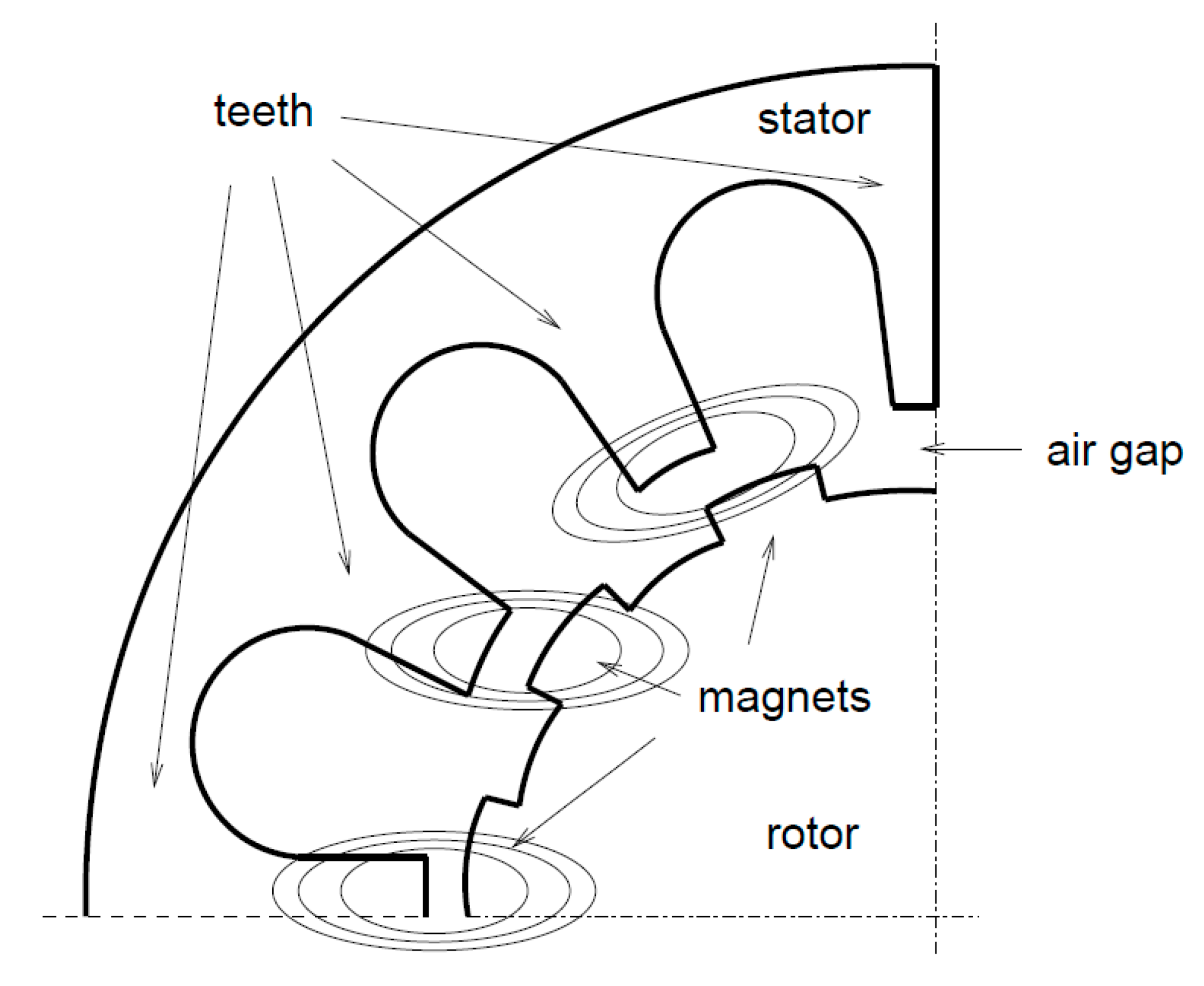
As intuitively represented in Figure 1, during the rotation of the motor axis, the variation of mutual position between the rotor and stator creates a variation of the air gap thickness. This means that the magnetic path in which the flux produced by the magnets is a function of the mutual position itself. This fact means that locally the intensity of this magnetic interaction between permanent magnets and stator teeth has a different intensity, depending on the angular position of the rotor axis.

Intuitively, the cogging torque can therefore be described by means of a periodic function with respect to the angular position of the rotor, with an angular period depending on the number of permanent magnets and the number of stator teeth. This means that from a modelling point of view the cogging torque can be represented as a general Fourier series with a certain number of harmonic terms as in Equation (1):

$$T_{cog}={\tilde{T}}_{cog}\left({\vartheta }_m\right)={\displaystyle \sum }_k{A}_{k}cos\left(k\frac{{\vartheta }_m}{{\vartheta }_p}+a_k\right)+B_{k}sin\left(k\frac{{\vartheta }_m}{{\vartheta }_p}+b_k\right)$$

(1)

$$T_{cog}={\displaystyle \sum }_k{C}_{k}sin\left(kZ{\vartheta }_m+{\phi }_k\right)$$

(2)

where ${\vartheta }_m$ represents the mechanical rotor axis position (absolute), ${\vartheta }_p$ represents the angular period of the cogging torque (function of the number of stator teeth and magnets in the internal structure of the motor) meanwhile with $A_k,B_k,a_k \mathrm{and} b_k$ are the harmonic series coefficients.

The characterization of the cogging torque with a deterministic model it is very helpful in our case. Indeed, a closed form model can be easily introduced in the dynamic model equations in order to apply the feedback linearization theory [5] and to compute a control laws vector which takes into consideration the cogging effect by the systematic operating procedure that characterizes such control technique. There are many works in literature in which is described a procedure to represent the cogging torque with a closed form modelling, starting for example from a FEM (finite elements analysis) model or Maxwell equation-based model, as in [6,7,8].

In our work reference is made to the model of the authors in [9] for the simplicity in the link between the number of stator teeth and the number of pole pairs. The angular period ${\vartheta }_p$ is a function of the stator teeth and pole pairs number. The angular period can be defined as ${\vartheta }_p=\frac{2\pi }{l.c.m\left(p,Z\right)}$, where p is the number of pole pairs and Z is the number of stator teeth. The internal architecture of a synchronous motor has a teeth number greater respect the number of pole pairs, so it is possible to assume that $l.c.m \left(p,Z\right)=Z$. The proposed model is that of Equation (2) where $T_j$ and ${\phi }_j$ are the $j^{th}$ amplitude and phase coefficient of Fourier development, $Z$ is the number of stator teeth of the Synchronous motor while ${\vartheta }_m$ is the mechanical angular position of the rotor axis.

As will be justified in the next sections, this type of modeling of the cogging phenomenon is very useful in the development of a control algorithm for its reduction, as it can be directly inserted into the dynamic model of the electric motor. It is intuitive from Equation (2) that to take advantage of the mathematical model of cogging it is necessary to have available the measurement of the angular position, from an encoder or from a resolver. In a sensorless architecture, direct measurement of the position of the rotor axis is not available, but only an estimate based on the mathematical model is available. This is what makes the following work interesting, namely the verification of the Cogging torque reduction by means of a control algorithm, which uses an electric drive with a structure without angular position or angular velocity sensors.

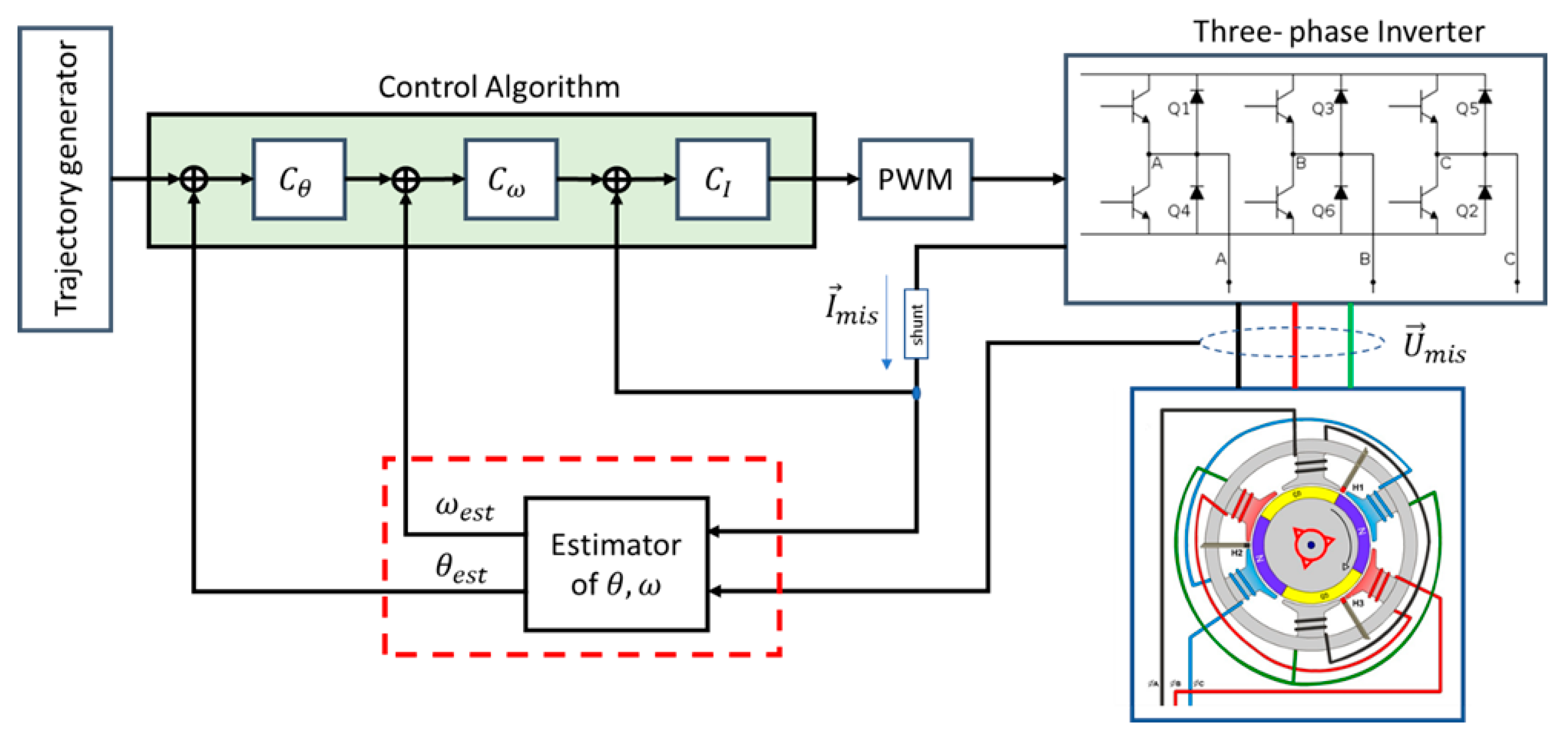
In a generic electric drive with sensor-less architecture [10], the project of a state observer is exploited, which provides an estimate of angular position and angular speed, based on the knowledge of the dynamic model of the motor itself and on the availability of direct measurements of current absorbed by the equivalent circuit and of supply voltage, deriving from appropriate sensors arranged in the three-phase inverter. The figure below shows a simplified schematic representation of a generic electrical drive with sensor-less architecture.

Figure 2 shows in a functional way the structure of a Sensorless electric power drive, in which it is noted how the observer of the state variables takes as inputs the direct measurements of voltage and current coming from the inverter (or equivalently from the motor phase), providing as output an estimate of position and angular speed of the rotor. There are many types of state observer so in the next section they will be briefly reported/described and explaining the selected one for this work.

3. State-of-Art on Cogging Torque Reduction

There are no other works about the usage of a sensor-less power drive system architecture for a synchronous motor with the goal of rotor axis position control including the effect of the cogging torque, exploiting the feedback linearization technique. Furthermore, there are very few works in literature regarding the rotor axis position control for electric power drive systems in which is exploited a sensor-less architecture, meanwhile are present a lot of works about the speed control with a sensor-less power drive system, in which is often required to track a slow variation reference signal. In the follow we report the state of the art relative to the reduction of the cogging torque through various control technique instead of physical modification in term of stator teeth shape and placing the permanent magnets inside the rotor iron structure. We report also various work about the design of control systems in which are combined a non-linear control technique and non-linear state observer. Furthermore, we report the works in literature regarding the position control with sensor-less architecture for synchronous power drive systems.

The first approach for reducing the cogging torque is the physical modification of the rotor and stator internal structure. For instance, the authors of [11] present three cogging torque reduction methods by using tangential displacement of stators, asymmetric rotor pole shaping, and a segment-twisted rotor. In [12], the influence on cogging torque of slot openings and tooth profile in axial-flux permanent magnet (PM) machines is presented, in order to propose a different opening angle. Reference [13] investigates the production tolerances and variations of the lamination and permanent magnet on the cogging torque of the SPM machine with mass production, in order to propose a helpful analysis and a reduction method based on stator caves modification. In [14] the influence of stator teeth shaping on cogging torque developed by radial flux permanent magnet brushless direct current (DC) motor is investigated in order to propose a different disposition and shape of the permanent magnets along the rotor surface. In [15] the authors present the optimization of cogging torque under pole shape changing with Taguchi method, response surface methodology, and genetic algorithm. The authors of [16] show a different disposition of the permanent magnets in order to reduce both the cogging torque and the torque ripple.

The algorithms regarding the reduction of the cogging torque effect on the rotor axis position exploiting physical modification have the limitation to require the replacing of the motor itself with a new one in the power drive system. Further the physical modifications are often expensive and require different modality in the fabrication phases.

Another approach which does not require the replacing of the motor in the drive system is to design a control algorithm able to absorb the effects of the magnetic interaction between rotor and stator in terms of rotor axis position.

In [17] the authors present an interesting Lyapunov-based method for the design of a non-linear control law in order to reduce both the cogging torque through one of the three descripted step of their algorithm, and the Stribeck effect exploiting a disturbance observer.

The authors of [18] describe a method based on minimizing a cost function that considers the flux linkage torque harmonics obtained from a discrete-time model of the machine, and furthermore it is proposed to mitigate the other source of torque ripple, known as cogging-torque, using a feed-forward signal applied to the torque control loop.

In [19] two different methods for the identification of the cogging torque in three-phase PM motors are presented, so the cogging torque map carried out from these methods is then used in a field-oriented control (FOC) algorithm to mitigate the ripple in speed and torque. In [20] a reduced order non-linear observer is designed to estimate the cogging torque, and the robustness analysis regarding the uncertainties is given for the proposed non-linear observer. A triple-step non-linear method is applied to derive a speed tracking controller, and then the robustness analysis against considered observation errors and lumped uncertainties is completed.

In [21] the authors propose a robust iterative learning control (ILC) scheme achieved by an adaptive sliding mode control (SMC) technique to further reduce the torque ripples and improve the anti-disturbances ability of the servo system. ILC is employed to reduce the periodic torque ripples and the SMC is used to guarantee fast response and strong robustness.

In [22] the authors propose a combination of model predictive control (MPC) and ILC to not only speed up the response time of the system but also effectively reduce the speed ripples. MPC updates the predictive model in real time through feedback and evaluates the system output and control rate according to the cost function.

As in [17,18,19,20,21,22], the majority of the works in literature approaches the cogging torque problem in the context of a speed control system, actually the presence of the cogging behaviour creates more problems in position control loop than in the speed one. This is due to the fact that the wavelike trend is more a problem in applications in which is required a high precision in rotor axis positioning. In the following, we report also some helpful works that describe the recent methodologies in rotor position control in which is implemented some cogging torque reduction techniques.

In [23], the authors consider a new structure of disturbance observer based on a zero-order disturbance observer and torque ripple table; in this way it is possible to accurately estimate the instantaneous disturbance torque by using the proposed disturbance observer.

In [24] is presented a non-linear control architecture based on feedback linearization technique which exploits knowledge on the cogging torque through the definition of a closed form modelling of it. The authors present the experimental results in terms of a desired position trajectory tracking followed by a parametric robustness analysis and a computational analysis for low-cost embedded platform implementation.

Furthermore, in the following we report some works useful in the presented one, in the context of sensor-less rotor axis positioning for generic synchronous permanent magnet machines.

In [25] is reported the classic usage of a discrete-time-domain EKF to a dq-axis of a stepper motor in order to control the rotor axis position in a sensor-less control system. In this paper the authors do not consider the effect of the cogging torque and cogging ripple.

Reference [26] presents a scheme for estimating the dominant cogging torque harmonics using a back-EMF estimator sensor-less controller, in which the experimental results show that over the expected range of system variation in viscous friction, the estimate will vary by less than 20%.

The authors in [27] used an interesting three-step procedure: first, the series self-inductance area difference method, in consideration of cogging torque produced by a field current, is adopted for identifying the initial position; second, the current pulse injection technique in the commutation point is proposed to detect the commutation moment at low speed; third, the terminal voltages are considered as vectors with a fixed phase difference, and the composed vector is rotated with varying rotor positions. In [28], the authors present sensor-less control of a low-speed permanent magnet synchronous machine with use of modified state observer, for torque ripple and cogging compensation. In [29] is implemented a non-linear control technique based on a continuous time domain EKF sensor-less architecture, comparing various model of the synchronous motor for the observer system design.

Other interesting work of the literature helpful to design our proposed solution are reported in the following for completeness.

In [30] the authors present an active disturbance rejection control (ADRC) based on the identification of the rotor position based on a high-frequency injection methodology. In [31] a sliding mode control for constant speed control is reported, exploiting a sensor-less architecture based on a linear Luenberger observer. In [32] a new high-speed sliding mode observer (SMO) is proposed for a Permanent Magnet Linear Synchronous Motor (PMLSM) based on the sliding mode variable structure theory in which sigmoid function is used for the SMO as a switching function of the control law, eliminating sliding mode chattering and improving its response rate. In [33] a classical usage of the extended Kalman filter in the context of a Proportional Integrative (PI)-cascade control sensor-less architecture is presented for constant speed control loop. In [34] another constant speed control, exploiting an innovative adaptive configuration of a Kalman filter (KF) with classic PI controller chain. In [35] is reported an interesting observability analysis of the $\alpha \beta -axis$ equivalent model of a Synchronous motor used in order to improve the performance of the sensor-less architecture based on EKF, in the start-up phase, which is critical for position estimation in surface permanent magnet motors. Lyapunov based techniques are also addressed in [36] with reference to the problem of estimation of rotor angular position. Sliding-mode observers for the same problem have been proposed in [37,38].

4. Design of the Control System

In this section we report in detail the control algorithm, used in one of our previous works [24] concerning the reduction of the cogging torque through a control technique, and the configuration chosen for the EKF, which is different from most of the works reported in the literature.

As a control technique we use FLC, whose use for this type of problems is widely discussed and justified. For the sake of completeness, the essential steps necessary for the reader to understand the procedure are given below.

As known from the theory of electrical machines, the model in dq axes is obtained by applying transformations of coordinates to the model in three-phase axes, with the goal to delete the dependence of the electromagnetic torque by the rotor axis positioning. In this way it is possible to reuse the control concept of a DC motor.

Below we report both the electrical dynamic model of a permanent magnet synchronous motor expressed in three phase axes and in dq axes, in Equations (3) and (4) respectively.

$$\left(\begin{array}{c}{u}_a\\ u_b\\ u_c\end{array}\right)=R_s\left(\begin{array}{c}{i}_a\\ i_b\\ i_c\end{array}\right)+L_{eq}\frac{d}{dt}\left(\begin{array}{c}{i}_a\\ i_b\\ i_c\end{array}\right)-p\omega k_{\phi }\left(\begin{array}{c}sin\left(p\vartheta \right)\\ sin\left(p\vartheta -\frac{2\pi }{3}\right)\\ sin\left(p\vartheta -\frac{4\pi }{3}\right)\end{array}\right)$$

(3)

$$\left(\begin{array}{c}{u}_d\\ u_q\end{array}\right)=R_s\left(\begin{array}{c}{i}_d\\ i_q\end{array}\right)+L_{eq}\frac{d}{dt}\left(\begin{array}{c}{i}_d\\ i_q\end{array}\right)+p\omega \left(\begin{array}{c}-L_{eq}{i}_q\\ L_{eq}{i}_d+k_{\phi }\end{array}\right)$$

(4)

In Equation (3), $u_a,u_b,u_c$ and $i_a,i_b,i_c$ represent the components of the voltage supply vectors and the current absorbed by the motor, respectively; $R_s$ and $L_{eq}$ are the resistance and equivalent inductance of the stator electric circuit; $p$ is the number of polar pairs; $k_{\phi }$ is the intensity of the magnetic field produced by the permanent magnets; $\vartheta$ and $\omega$ are the angular position and the angular (mechanical) speed of the rotor instead.

The mechanical equilibrium has the same formalism both in the case of a model written in three-phase axes and in equivalent dq axes, as shown below:

$$\left(\begin{array}{c}{u}_d\\ u_q\end{array}\right)=R_s\left(\begin{array}{c}{i}_d\\ i_q\end{array}\right)+L_{eq}\frac{d}{dt}\left(\begin{array}{c}{i}_d\\ i_q\end{array}\right)+p\omega \left(\begin{array}{c}-L_{eq}{i}_q\\ L_{eq}{i}_d+k_{\phi }\end{array}\right)$$

(5)

In Equation (5) we indicate with $J_m$ the moment of inertia of the rotor and with $\beta$ the coefficient of rotation friction of the axis; $T_{em}$ is the electromagnetic torque, completely due to the electromechanical conversion of energy.

In this last equation $T_{cog}$ is the one introduced in Equation (2), while $T_{em}$ has different expressions depending on the frame of reference. In particular, if it refers to the model in three-phase axes its expression is $T_{em}^{abc}=-p{k}_{\phi }{{\displaystyle \sum }}_k{i}_{k}sin\left(p\vartheta -2\pi \left(k-1\right)/3\right)$, while in dq axes it is $T_{em}^{dq}=\frac{3}{2}p{k}_{\phi }{i}_q$.

In this work we consider a SPM architecture of the synchronous machine, but nothing changes in the design control procedure if an IPM internal structure of the machine itself is considered. The only thing that changes in the machine modelling is the formal expression of the electromagnetic torque in which must be included the contribution of the anisotropy.

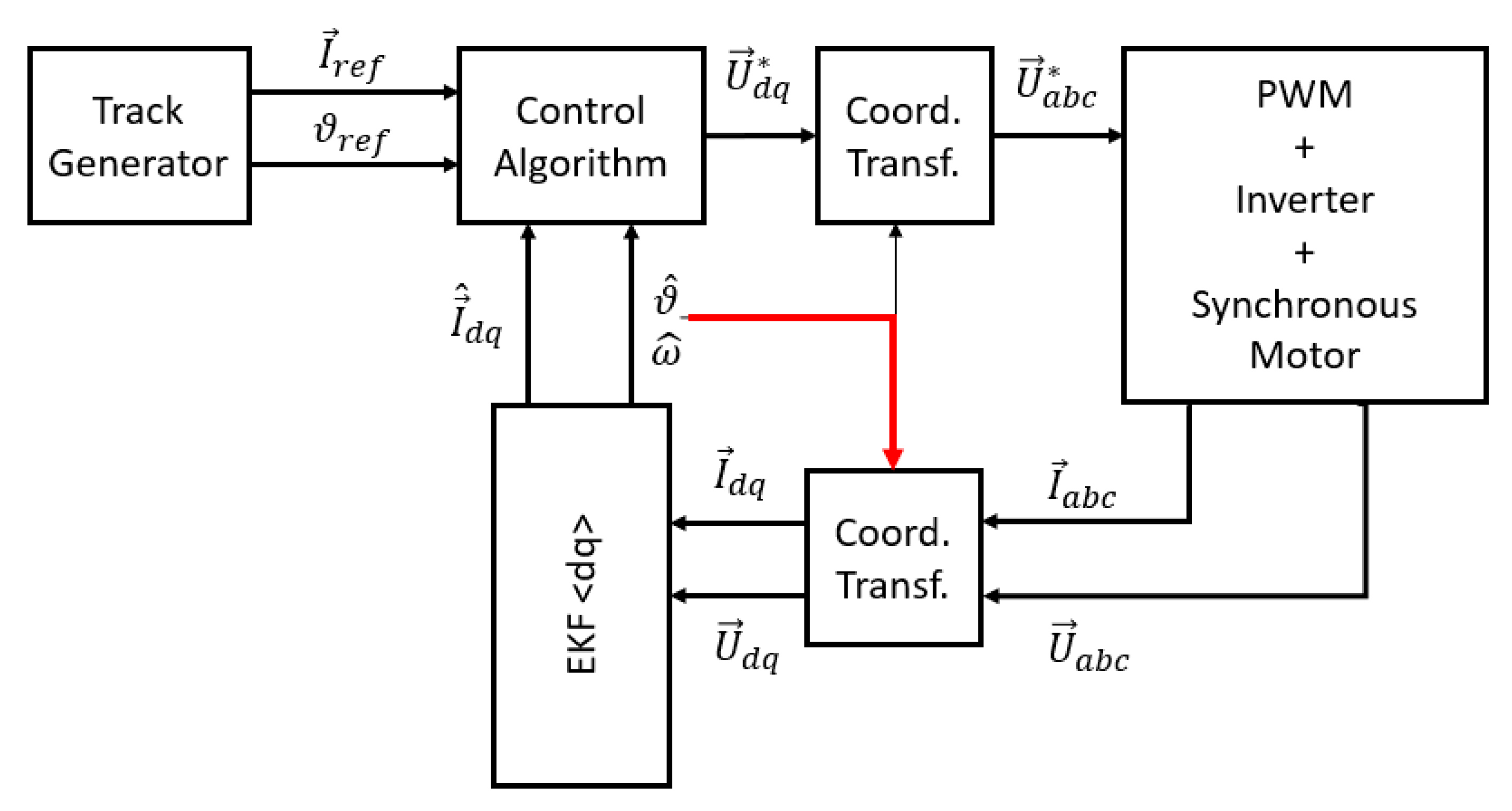
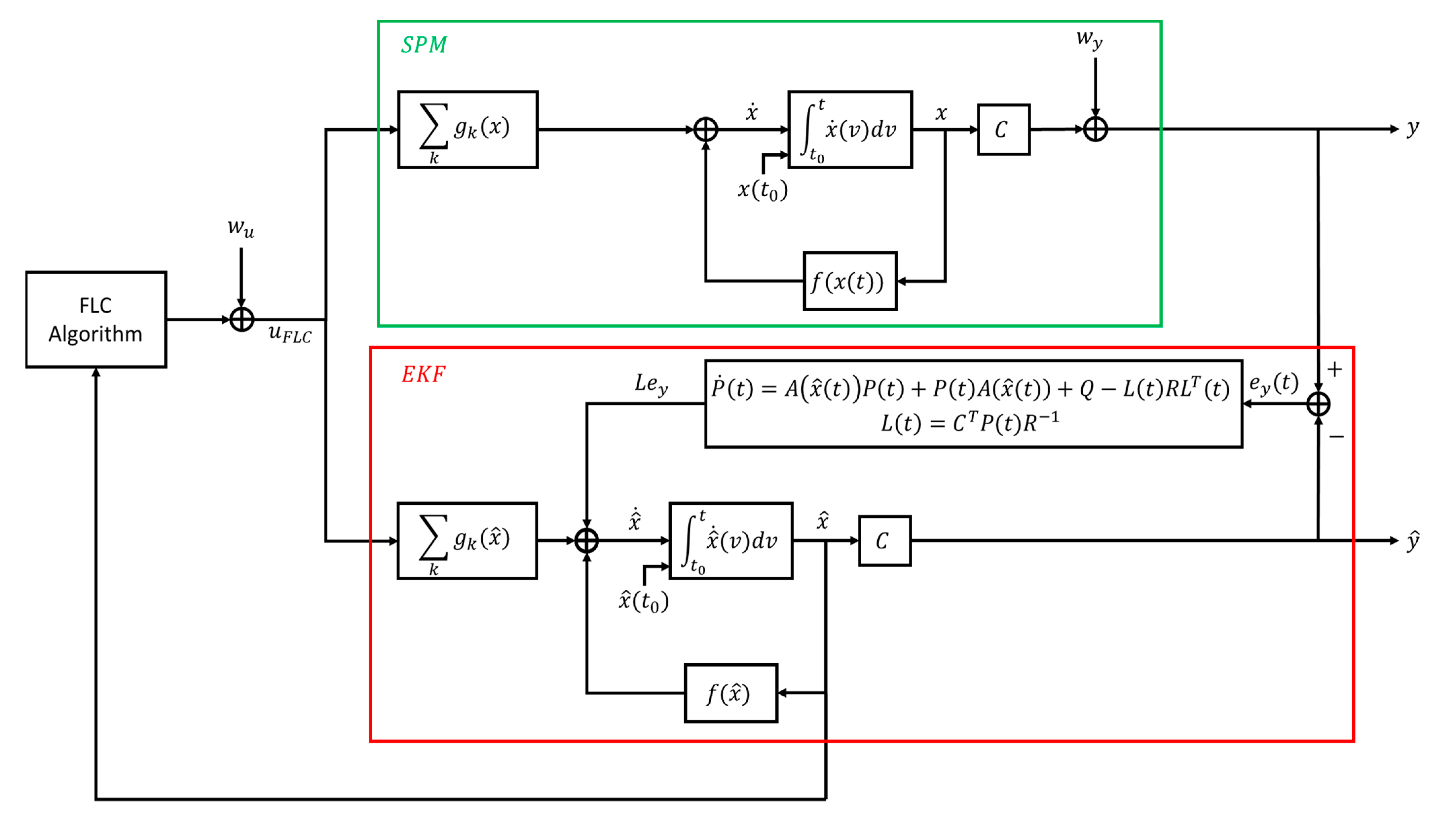
In this work, the dq axis model was used for the design of the control laws, while for the design of the EKF, reference was made to the three-phase axis modelling. As shown schematically in Figure 3, using as a reference model for the design of the EKF that in the dq axes of the motor, it is necessary to make an estimated position feedback on the block of transformation of coordinates that maps the three-phase components of current and voltage into components of the dq frame.

In Figure 3 the red line highlights the reaction of the estimated state. From a conceptual point of view, consistent with Kalman filter theory, measurable inputs and outputs must be provided at the input of the estimation system, and in fact with the architecture described in Figure 3 the EKF takes at the input the result of the transformation of coordinates on the measurement of current and voltage, which is a function of the estimated position, which in fact is not a true measurement.

Moreover, the presence of the estimated position feedback can be a problem in the use of a continuous time domain EKF, as it has to use the estimate provided at the generic instant of time $t$, both as input for the control system and to supply the inputs to the filter itself, and this fact could be a reason for the presence of algebraic loops.

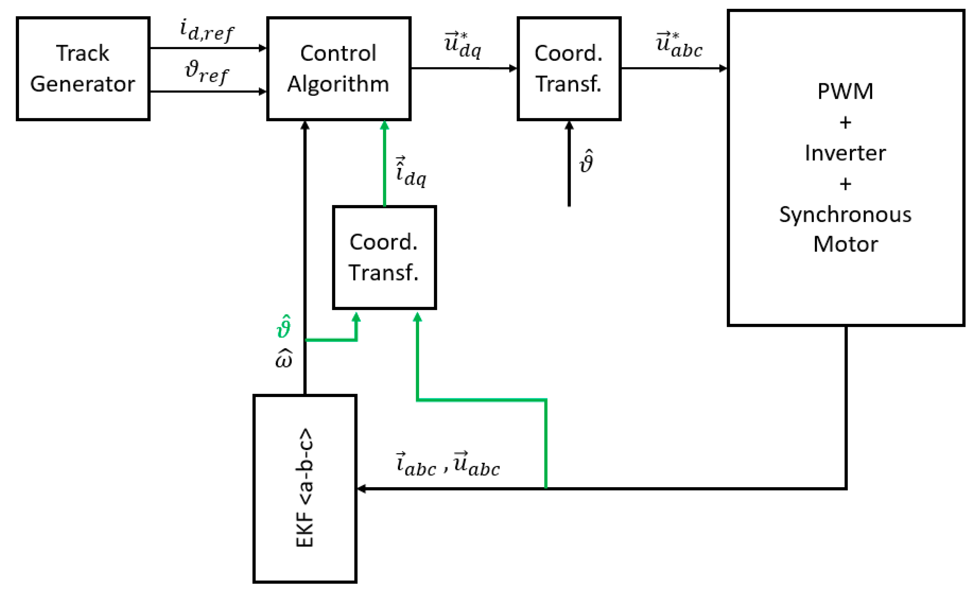
The configuration we propose, schematically represented in Figure 4, foresees the use of the model expressed in three-phase axes for the realization of the EKF. In this way, direct measurements of supply voltages and currents absorbed by the stator phases have an input of the filter. Moreover, the problem of unwanted feedback described previously is solved, since, as shown by the green connections in Figure 4, the transformation takes place downstream of the observer.

Also from a logical point of view it makes more sense because it is possible to supply the control system with the quantities necessary to calculate the algebraic relations designed by FLC only after the calculation of the transformation of coordinates from three-phase axes to dq axes for what concerns the currents.

Clearly using the architecture shown in Figure 4 we pay the price of a higher number of equations within the reference model, as can be seen from Equations (3) and (4), the dynamics of the system in three-phase axes is made up of a non-linear differential equation more than the model in dq axes. In the following EKF constituent equations are used. In particular, it should be noted that instead of the Jacobian matrix calculated in the current estimated state vector, a linear regressor was used in the same estimated state vector, to use it in the Riccati equation.

This should help in the istantaneous correction of the EKF gain matrix, based precisely on the measurable and predicted output error weighed with that matrix. In general, mathematical models of Lagrangian electromechanical systems, such as an electric motor or a robotic system or even a vehicle, can be rewritten in the state form of a non-linear and in particular in “affine in the control” form, where the contribution of the control vector components can be expressed as a linear combination of the control variables whose weights are the control vector fields, and there is a drift component of the differential equations. In Equation (6) with f(x,u) we indicate the generic vector field that defines the set of differential equations in the form of Cauchy; with f(x) the drift vector field, with $g_k\left(x\right)$ the $k^{th}$ control vector field and $u_k$ the $k^{th}$ component of the control vector; A(x) is the linear regressor with respect to the state variables.

$$\dot{x}=f\left(x,u\right)=f\left(x\right)+{\displaystyle \sum }_k{g}_k\left(x\right)u_k=A\left(x\right)x+{\displaystyle \sum }_k{g}_k\left(x\right)u_k$$

(6)

$$\begin{gathered} \widehat{\dot{x}}=f\left(\widehat{x}\right)+{\displaystyle \sum }_k{g}_k\left(\widehat{x}\right)\left(u_k+w_u\right)+L\left(y-C\widehat{x}\right) \\ y=Cx+w_y=\left[\begin{array}{cc}{I}_{3x3}& 0_{3x2}\end{array}\right]x+w_y \\ \widehat{y}=C\widehat{x} \\ \dot{P}=A\left(\widehat{x}\right)P+P{A}^T\left(\widehat{x}\right)+Q-LR{L}^T \\ L=C^{T}P{R}^{-1} \end{gathered}$$

(7)

In Equation (7) we have indicated with $\widehat{x}={[{\widehat{i}}_a {\widehat{i}}_b {\widehat{i}}_c \widehat{\vartheta } \widehat{\omega }]}^T$ the estimated vector of state and with $\widehat{y}={[{\widehat{i}}_a {\widehat{i}}_b {\widehat{i}}_c]}^T$ the vector of estimated exits. The link between state variables and outputs for the observer is the same as for the deterministic model of the motor, through C matrix.

The inputs of the EKF are all the measurable quantities, in particular the currents supplied by the motor and the voltages that supply it.

In Equation (7) with L the gain matrix of the EKF is indicated, which serves to weigh and map the contribution of the error $e_y$ in the dynamics of the estimated state $\widehat{x}$; P is instead the covariance matrix of the estimated state, solution of the Riccati matrix equation, deriving from a problem of unconstrained optimization and in particular of minimizing the average quadratic deviation of the error; Q and R are the covariance matrices of the additive noise signals at the output and at the input to the process, respectively.

Furthermore, for the additive model of noise signals for voltage and current measurements, Gaussian noise signals of type $w_u ~N\left({\mu }_u,{\sigma }_u^2\right)\equiv N\left(0,2^2\right)$ were taken into account for voltage measurements (process input) and $w_y~N\left({\mu }_y,{\sigma }_y^2\right)\equiv N\left(0,5^2\right)$ for current measurements (measurable state variable) were taken into account. Figure 5 shows the high-level schematization of the architecture of the sensor-less electric drive, deriving from the constitutive equations reported in the set in Equations (6) and (7). Below we report the essential steps of the operative procedure, necessary to obtain the expression of the control vector, exploiting the feedback linearization theory. Starting from the generic state form of Equation (6), fixed the control outputs $y_i=h_i(\overrightarrow{x})$, the operating procedure consists in identifying the relative degree ${\mu }_i$ of each one, indeed the number of derivations necessary to obtain an expression as a function of at least one component of the control vector. Once the expression of the ${\mu }_i^{th}$ derivative has been obtained, the linearization condition is imposed, which consists in requiring that the new input-output ratio is linear, and more precisely that it is equivalent to a chain of integrators of equal order to the relative degree.

$$\frac{d^{{\mu }_i}{y}_i}{d{t}^{{\mu }_i}}=L_f^{{\mu }_i}{h}_i\left(\overrightarrow{x}\right)+{\displaystyle \sum }_{k=1}^m{L}_{g_k}{L}_f{h}_i\left(\overrightarrow{x}\right)u_k$$

(8)

From the previous equation, applying the reasoning described above, calling $v_i$ the $i^{th}$ component of the new control vector, the condition to be imposed is the following:

$$\frac{d^{{\mu }_i}{y}_i}{d{t}^{{\mu }_i}}=v_i \to Y_i\left(s\right)=\frac{V_i\left(s\right)}{s^{{\mu }_i}}$$

(9)

Extending to all control outputs, we clearly obtain a total number of equations equal to ${\mu }_z={{\displaystyle \sum }}_{k=1}^s{\mu }_k$, which in matrix form take the following form:

$$\left[\begin{array}{c}\frac{d^{{\mu }_1}{y}_1}{d{t}^{{\mu }_1}}\\ ⋮\\ \frac{d^{{\mu }_s}{y}_s}{d{t}^{{\mu }_s}}\end{array}\right]=\left[\begin{array}{c}{L}_f^{{\mu }_1}{h}_1\\ ⋮\\ L_f^{{\mu }_s}{h}_s\end{array}\right]+\left[\begin{array}{ccc}{L}_{g_1}{L}_f^{{\mu }_1-1}{h}_1& \cdots & L_{g_m}{L}_f^{{\mu }_1-1}{h}_1\\ ⋮& \ddots & ⋮\\ L_{g_1}{L}_f^{{\mu }_s-1}{h}_s& \cdots & L_{g_m}{L}_f^{{\mu }_s-1}{h}_s\end{array}\right]\left[\begin{array}{c}{u}_1\\ ⋮\\ u_m\end{array}\right]=L\left(x\right)+E\left(x\right)\overrightarrow{u}=\overrightarrow{v}=\left[\begin{array}{c}{v}_1\\ ⋮\\ v_s\end{array}\right]$$

(10)

In accordance with the theory, a state base change is operatively described in this way.

To simplify, let us assume that the total sum of the relative degrees is equal to the size of the starting state space (${\mu }_z=n$). Moreover, in the case under examination, where basically a FOC check is performed, by imposing a zero-current reference of quadrature axis and a trajectory reference for the angular position, the E(x) matrix is square and fully invertible. In the case of position control let us talk about exact feedback linearization, since the new status vector has the same size as the previous one. In the new base, the dynamics are in linear form: $\frac{dz\left(t\right)}{dt}=A_{z}z\left(t\right)+B_{z}v\left(t\right)$, with z(t) the new state vector. and, in addition, by construction, the pair $\left(A_z,B_z\right)$ is completely reachable. According to the latter observation, the new vector $v\left(t\right)$ can be obtained with one of the linear control techniques such as pole repositioning, Linear Quadratic Control (LQR) control or $H_{\infty }$ control. In the case of synchronous motor control, the design of the control law is done according to the dq-axis model, which consists of four state equations (two electrical equilibrium and two mechanical equilibrium) and two control variables. As already mentioned, we consider as control outputs $h_1=i_d$ and $h_2=\vartheta$.

$$\begin{array}{cc}{u}_{dq}=E^{+}\left({\widehat{x}}_{dq}\right)\hfill & \left(v_{dq}-S\left({\widehat{x}}_{dq}\right)\right)+Ker\left(E\left({\widehat{x}}_{dq}\right)\right)\hfill \\ & ={\left[\begin{array}{cc}{L}_{g_1}{L}_{f_{dq}}^{{\mu }_1-1}{h}_1\left({\widehat{x}}_{dq}\right)& L_{g_2}{L}_{f_{dq}}^{{\mu }_1-1}{h}_1\left({\widehat{x}}_{dq}\right)\\ L_{g_1}{L}_{f_{dq}}^{{\mu }_2-1}{h}_2\left({\widehat{x}}_{dq}\right)& L_{g_2}{L}_{f_{dq}}^{{\mu }_2-1}{h}_2\left({\widehat{x}}_{dq}\right)\end{array}\right]}^{+}\left(v_{dq}-\left[\begin{array}{c}{L}_{f_{dq}}^{{\mu }_1}{h}_1\left({\widehat{x}}_{dq}\right)\\ L_{f_{dq}}^{{\mu }_2}{h}_2\left({\widehat{x}}_{dq}\right)\end{array}\right]\right)\hfill \\ & +Ker\left(E\left({\widehat{x}}_{dq}\right)\right)\hfill \end{array}$$

(11)

In Equations (8)–(11) is reported the expression of the control vector obtained with the Feedback Linearization technique, designed based on the motor model expressed in dq axes, $u_{dq}$; ${\widehat{x}}_{dq}$ is the estimated state vector after the transformation of coordinates based on the angular position $\widehat{\vartheta }$ estimated by the EKF; $f_{dq}$ and $g_1,g_2$ are the drift and control vector fields, respectively, for the model in dq axes rewrites in state-form; $v_{dq}$ is the control vector in the base of the state vector expressed by $z={\left[\dots h_i L_f{h}_i \dots L_f^{{\mu }_i-1}{h}_i\dots \right]}^T$; $h_1,h_2$ are in general the control outputs, which in this case are the direct axis current $i_d$ and the angular position $\vartheta$. It is verified that in the specific case the relative degrees are ${\mu }_1=1$ and ${\mu }_2=3$, which represent the number of temporal derivatives necessary to obtain, starting from $h_1$ and $h_2$, expressions containing both components of the control vector.

Finally, with the terms $L_f{h}_k,L_{g_i}{L}_f^{{\mu }_k}{h}_k,L_{g_k}{h}_i$ we indicate the lie-brackets, necessary to define the operating procedure for the calculation of $u_{dq}$, in accordance with the non-linear control theory.

5. Simulation Results

In this section are reported and described the results in terms of simulation in Matlab and Simulink environments, and a direct comparison with the sensorized architecture case in terms of computational complexity is made using the Simulink Profiler. It is also reported an analysis of robustness to parametric variations both respect to the initial conditions of the EKF and with regard to the coefficients of the mathematical model of the engine. For completeness, the characteristics of the synchronous motor used and of the cogging torque model are reported in

Table 1. Mathematical model coefficients.

Model Parameter	Values
$R_s\left(stator resistance\right)$	$3.3 \mathrm{Ohm}$
$L_{eq}\left(stator inductance\right)$	$50 \mathrm{mH}$
$k_{\phi }\left(pm flux intensity\right)$	$0.5 \mathrm{Wb}$
$J_m\left(rotor inertia\right)$	$0.02 {\mathrm{Kgm}}^2$
$p\left(pole pair\right)$	$3$
$\beta \left(friction coefficient\right)$	$0.01 \mathrm{Ns}/\mathrm{m}$

,

Table 2. Operating parameters of the motor.

Data Sheet Parameters	Values
$P_n$ (Nominal Power)	$15 \mathrm{k}\mathrm{W}$
${\omega }_n$ (Nominal Speed)	$1500 \mathrm{r}\mathrm{p}\mathrm{m}$
${\omega }_{max}$ (Maximum Speed)	$2000 \mathrm{r}\mathrm{p}\mathrm{m}$
$T_n$ (Nominal Torque)	$95.5 \mathrm{N}\mathrm{m}$
$T_s$ (Stall Torque)	$230 \mathrm{N}\mathrm{m}$

and

Table 3. Cogging mathematical model parameters.

Harmonic Expansion Coefficients	Values
$T_1$	$4.85 \mathrm{N}$
$T_2$	$2.04 \mathrm{N}$
$T_3$	$0.3 \mathrm{N}$
$T_4$	$0.006 \mathrm{N}$
${\alpha }_1$	$0.009 \mathrm{rad}$
${\alpha }_2$	$0.01 \mathrm{rad}$
${\alpha }_3$	$0.017 \mathrm{rad}$
${\alpha }_4$	${\alpha }_3$

.

The following is the result of trajectory tracking for the angular position of the rotor, which is the main task. Furthermore, the results of the estimation of the measurable status variables (the currents in three-phase axes) and of the angular speed, which is the second output of the EKF of interest for the completion of the control loop, are reported.

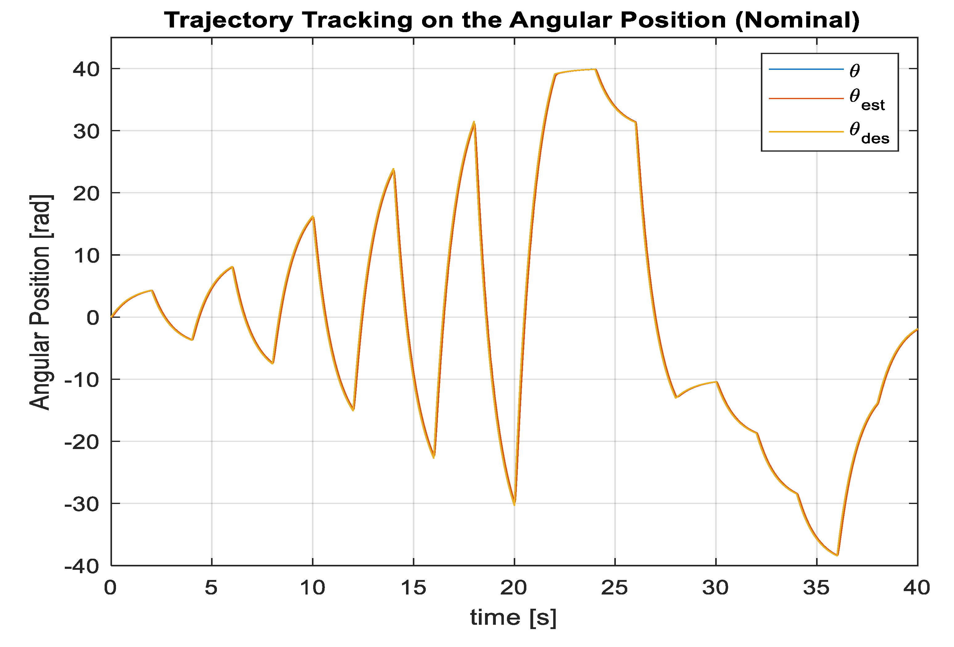
Figure 6 shows the result of the trajectory tracking concerning the position control loop. The desired trajectory is a non-trivial trajectory (not the classic step or a trapezoidal signal), to show that the result does not depend on the choice of reference.

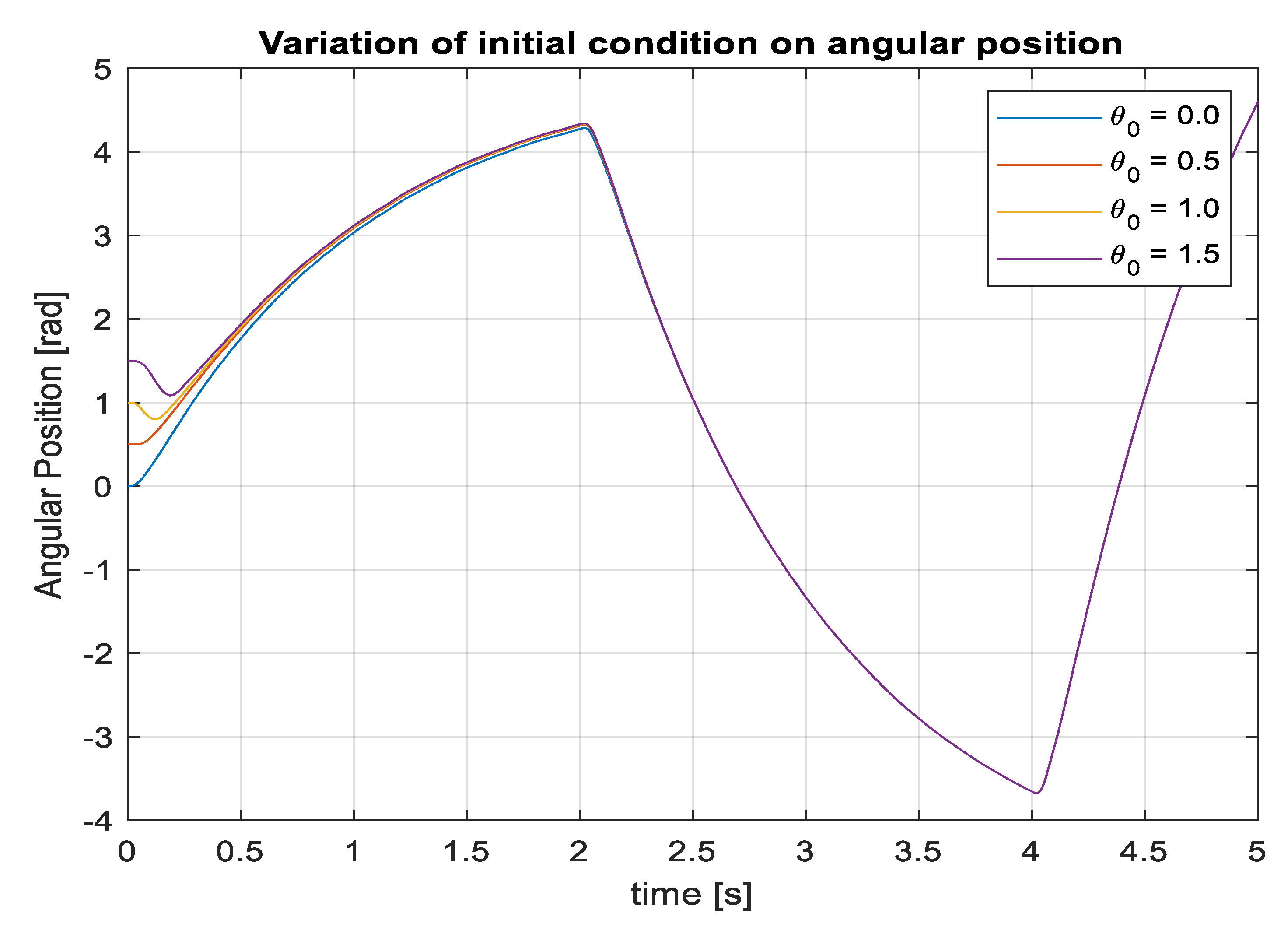
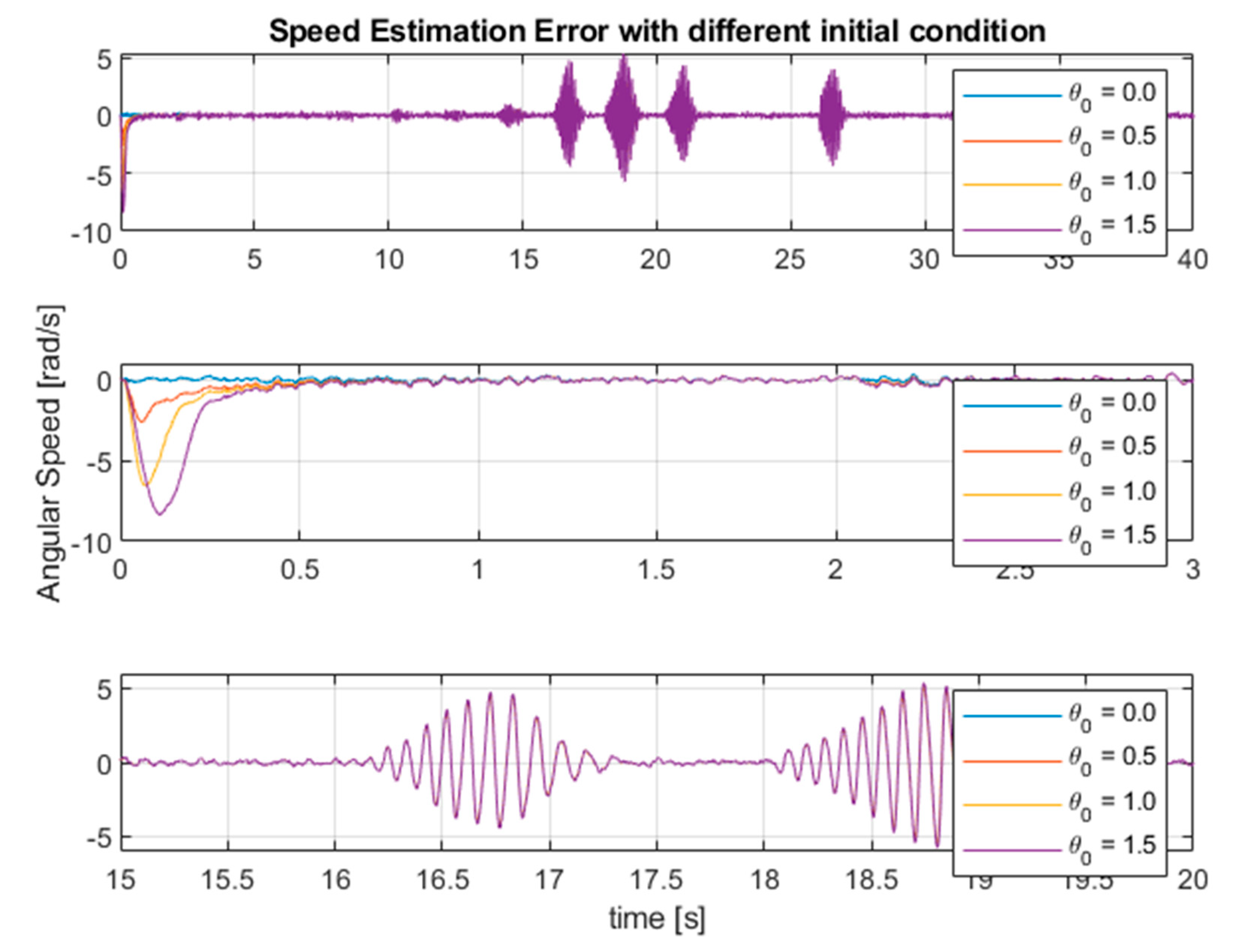
The figure shows the result of reclosing the control loop with variables estimated by the EKF but with initial conditions identical to those of the mechanical equilibrium. To verify that the good result achieved does not depend on the difference between the initial conditions of the process to be controlled and those of the filter, Figure 7 shows the trajectory tracking when the initial conditions vary.

The fact that the performance of a Kalman filter also depends on the initial conditions of the filter is also easily verified from a formal point of view, since the dynamics of the error of the estimated state can be made autonomous through the “error-corrector” structure of the EKF itself, but the solution depends on the initial condition of the error vector on the state estimation, which is exactly the difference between the initial conditions of the process and the initial conditions of the EKF.

This reasoning is even more relevant in the case of non-linear systems as the principle of eigenvalue separation is not generally guaranteed.

As expected, for relatively long periods of time the effect of the initial conditions has practically no influence on the performance of $\vartheta$, while in transient phase it is possible to appreciate a different behavior depending on the initial condition from which the motor starts. In any case, the effect is exhausted in fractions of a second, as shown in Figure 7.

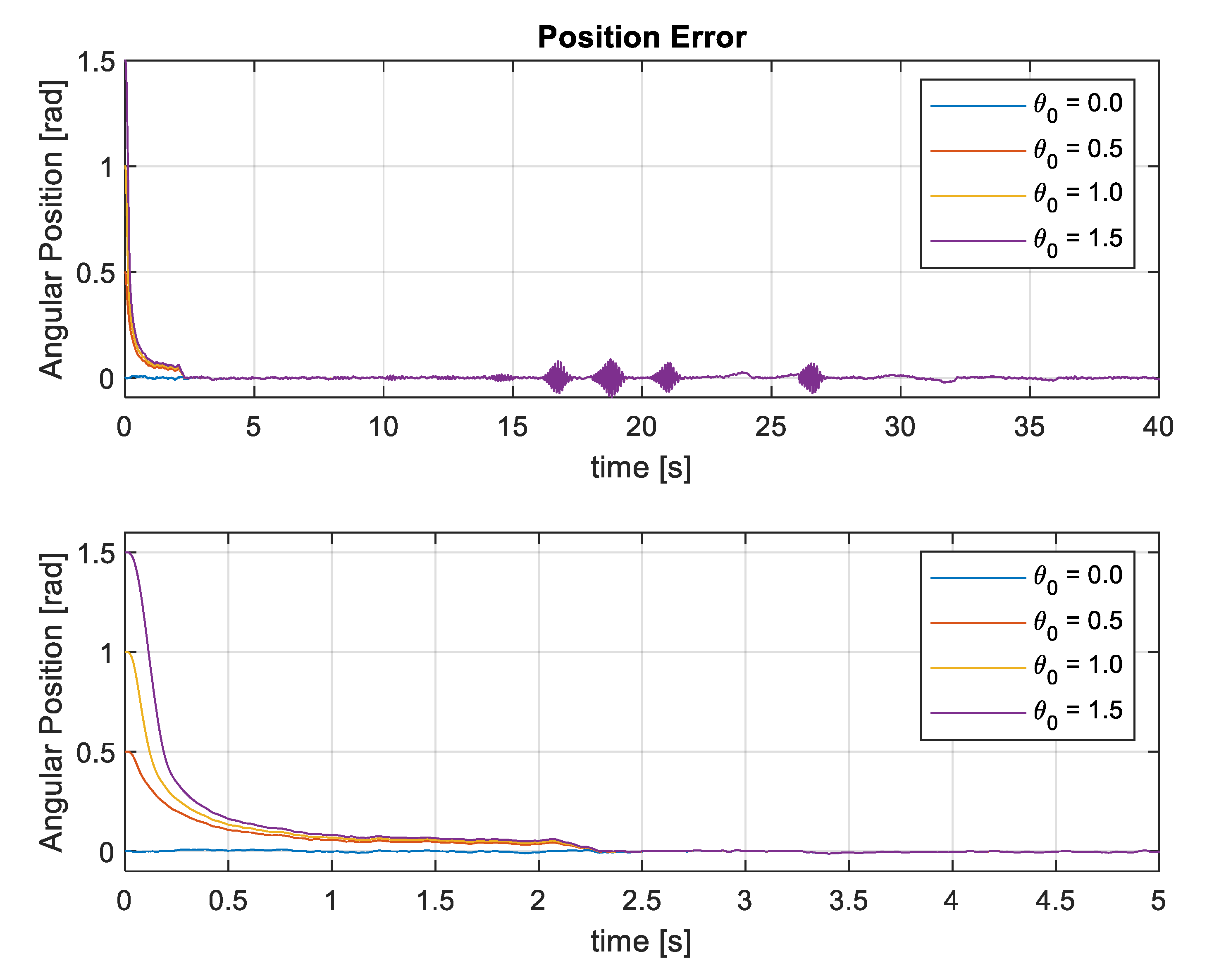
Figure 8 shows in detail the estimation error of the angular position. It can be seen that the error converges with the variation of the initial conditions of the model of the electric motor.

The error converges asymptotically as expected. In the points where the reference signal has a discontinuity of the derivative, however, there is a limited oscillatory trend.

This is certainly due to the settling transient in the error dynamics, which is compensated in a finite time, through the "error-corrector" dynamics of the estimated state based on the adaptation of the Riccati equation to the error variation itself. As shown below, in Figure 9 and Figure 10, this wave pattern also affects the estimated speed. However, in local transients, in correspondence with the more rapid changes in the reference signal, the error is more than acceptable. In fact, there is an error of a few tenths of a radian when the position is required to be around 30/40 radians for the position, while for the speed at such points there is an error of a few radians/second when the speed is around 40/50 radians/second. It is probable that the relative error on the velocity is greater than that of the position because a derivation operation is undertaken.

Moreover, it is verified that the estimation error does not exceed after the transitory phase an absolute value of more than about 6 degrees.

Figure 9 shows the result of the estimate provided by the EKF in terms of the mechanical angular speed of the rotor axis, as it represents the second variable not directly measurable necessary to close the control loop. The figure compares the angular speed of the motor and the speed at the output of the EKF, with which the control loop is closed. Unlike the angular position control loop where it is possible to make a comparison with the desired reference signal, in the case of angular speed it is not possible because with this choice of control technique a reference is not imposed for the speed loop, but the desired trends are set only for the position and for the direct axis component of the current.

Figure 10 (top) shows the result of the estimation of the angular velocity of the rotor axis, as the initial conditions of the rotor position relative to the mechanical dynamic equilibrium vary.

In Figure 10 (middle) and Figure 10 (bottom) are also reported in detail the transient phase where it is highlighted the contribution of the different initial condition of departure and the detail of the phases in which there are discontinuities in the derivative of the angular position reference.

The figures below show the estimated results for the other estimated state variables as well.

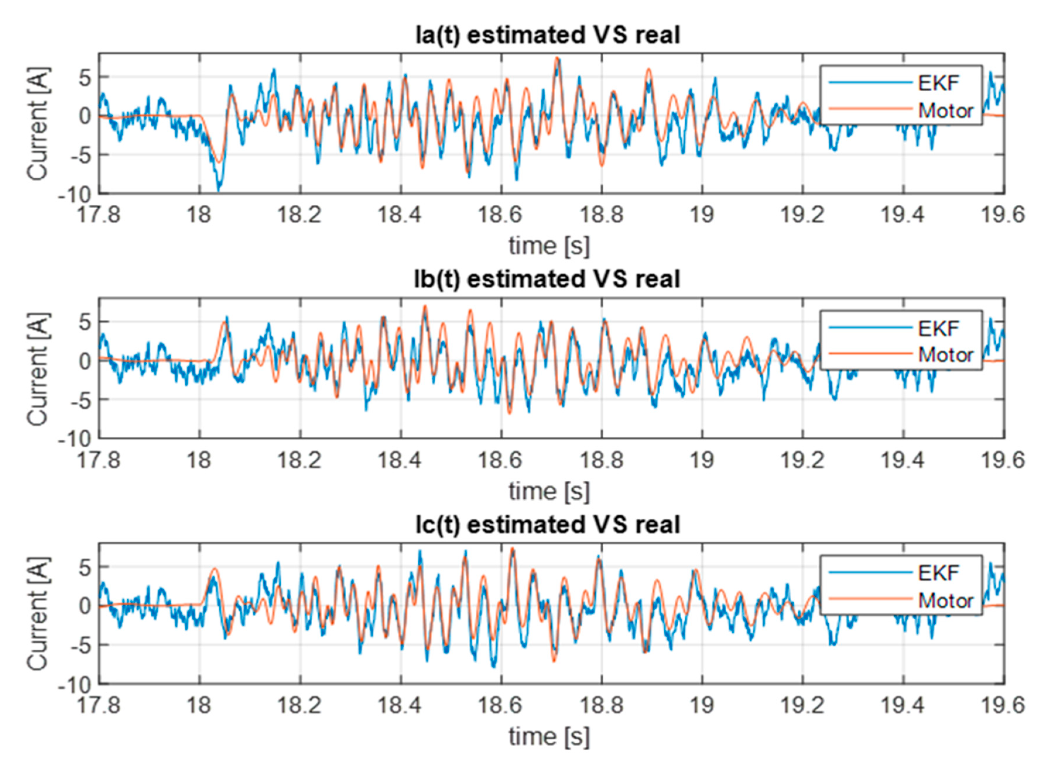
Figure 11 shows the result of the estimate provided by EKF for the current vector components in three-phase axes. The currents in three-phase axes are the components of the estimated state vector that are directly measurable.

The effect of the change in initial conditions is not reported as it is not very appreciable. The analysis of the variation of initial conditions with respect to the dynamics of the currents has little effect on the overall control loop behavior and is not reported.

Finally, Figure 12 shows the result of zero reference tracking for the direct axis current component in relation to the equivalent synchronous motor modeling.

In the following, we present a computational cost analysis based on the usage of the SW instrument, the Simulink profiler provides by MathWorks. In our case the complexity of the new global architecture must keep into account both the complexity of the non-linear control laws and the complexity due to the estimation system.

Intuitively, it is expected that the complexity substantially increased by the fact that the EKF is based on the resolution of both a vector differential equation (for the estimation of the $\widehat{x}$) and a matrix differential equation (the Riccati one).

In

Table 4. Summary from the profiler.

Summary Profiler Field	Value
$T_{rt}$	$2741.70 \mathrm{s}$
$N_{bm}$	$918$
$N_{im}$	$9$
$N_{mm}$	$13$
$N_{nsm}$	$46$
$C_p$	$30 \mathrm{ns}$
$C_s$	$3800 \mathrm{MHz}$

, $T_{rt}$ is the total recorded time, that is the total time required to simulate the model; $N_{bm}$ is the number of block methods, that is the number of invocations of block-level functions (e.g., output()); $N_{im}$ is the number of internal methods, which is the total number of invocations of system-level functions (e.g., model execute); $N_{nsm}$ is the total number of invocations of nonvirtual subsystem functions; $C_p$ and $C_s$ are the clock precision and clock speed, respectively, with respect to the platform on which the simulation is undertaken. The testing platform was a double core Intel® Core—i3-6300.

In the

Table 5. Complexity summary.

Functional Block	Time		Calls	Time/Call	Self-Time
Non-Linear Control	43.8672	1.6%	400036	$~$0.0001184	30158.7	1.1%
Kalman Filter	265,047	9.7%	2800221	$~$0.0000947	137.578	5.0%

, Time field means the total time spent executing all invocations of the specific function as an absolute value and as a percentage of the total simulation time; Calls field means the number of time the specific function was invoked; Time/Calls field represents the average time required for each invocation of the specific function, including the time spent in functions invoked by the function itself; and Self-Time field represents the average time required to execute the specific function, excluding time spent in functions called by this function.

As expected, the complexity of the global architecture is enough to suggest that the implementation on a low-cost platform as Arduino Uno, with an Atmel ATMEGA328 8-bit MCU, FLASH Memory 32KB, SRAM Memory 2KB, EEPROM Memory 1KB and Clock Speed 16 MHz, cannot be possible.

This consideration derives from that fact that with a percentage complexity amount (in terms of Simulink Profiler release) of 1.3%, the equivalent native language program sketch on the Arduino used around 20% of the space available for programs. Hence, it is reasonable that with a global percentage complexity (non-linear control and EKF) around 11%, the equivalent program in Arduino language will be more than the total capability of the Arduino itself.

6. Conclusions and Future Works

Summarizing, in this work we have presented the methodology for the project of a non-linear control algorithm inserted in an observed-based architecture with the goal to adsorb the unwanted wavy behavior caused by the intrinsic cogging phenomenon. An explanation of the different configuration of EKF that can be used is presented, with the aim to highlight some issues in the usage of a “dq-EKF” configuration for the estimation of the unmeasurable physical quantities. The “abc-EKF” is justified from an intuitively but also technical point of view as a better solution particularly in the case of continuous time domain implementation and used in the context of the cogging torque. The experimental results are presented with simulation of a classical trajectory problem in terms of desired rotor positioning as reference signal to follow. Results are presented with respect to a non-trivial rotor position desired signal. Furthermore, an analysis in term of algorithm complexity through the usage of SW tool, such as the Simulink Profiler is reported, which suggests implementing the observer-based non-linear control on more opportune low-cost platform, due to the fact that Arduino is not able to support the required throughput and memory space. Basically, this work is a proof of concept of the fact that our control algorithm is capable of absorbing, at least partially, the cogging torque effects also in case of sensor-less architecture. As a future extension of our work it will be interesting to compare the proposed solution with other types of observer-based estimation systems, such as machine-learning based algorithms or sliding mode/Utkin state observer. Another interesting extension to our work will be to exploit the learning concept both for the on-line estimation of the cogging torque as an output disturbance signal and to make adaptive our non-linear control algorithm. The focus of the paper was more on the theoretical and algorithmic part, verified by model-based design and simulations activities. Physical implementation of the electric drive with a low-cost electronic control unit implementing the proposed control strategy, and hence the availability of experimental measurement, is also part of future works.