On Obtaining Energy-Optimal Trajectories for Landing of UAVs

Abstract

The optimization issues connected to a landing task of an unmanned aerial vehicle are discussed in the paper, based on a model of a mini-class drone. Three landing scenarios are considered, including minimum-time landing, landing with minimum energy consumption, and planned landing. With the use of classical dynamic programming techniques, including the minimum principle of Pontryagin, as well as the calculus of variations, the optimal altitude reference trajectories are found, to form the altitude control system in such a way as to mimic the profile of the reference trajectory by the actual altitude of the UAV. The simulation results conducted with the use of the Simulink Support Package for Parrot Minidrones verify the correctness and effectiveness of the method, and open the research directions for further analysis, especially to tune altitude controller in a way, as to track the reference profile. Up to this point, optimization tasks considered in the literature, with respect to the drones, were connected to swarm formation optimization, optimization of the take-off process or landing process limited to optimal path planning. This paper thus considers a new topic in the field.

1. Introduction

Recent years have brought an increased popularity of unmanned aerial vehicles (UAVs), which, due to their increasing popularity in the market, have wider and wider applicability areas, ranging from pure recreation to scientific research. The latter implies the need to improve control algorithms which govern behaviour of UAVs to increase their safety and reliability. This can also be understood in the context of energy consumption efficiency.

A variety of tasks carried out by UAVs is a challenge for control engineers [1] responsible for controller tuning of drones. During in flight conditions, the UAVs are required to perform both agile, as well as precise maneuvers, also including maneuvers in formations of UAV, making the issues more complicated [2]. However, during the landing process, the situation is different, and the drones should closely abide some reference trajectories to achieve efficient landing with respect to some performance indices. In addition, at any stage of the flight, it might be necessary to land due to environmental issues, or low battery state, and to execute the flying scenario on the basis of, for example, some state machine.

In 2016, the Department and Aeronautics and Astronautics (AeroAstro) from Massachusetts Institute of Technology (MIT) designed the Simulink Support Package for Parrot Minidrones as Matlab’s add-on [3]. The software enables one to design, simulate and test control strategies using real UAVs, and is dedicated to Rolling Spider and Mambo drones of Parrot. It can be also used, as in the current paper, to perform model-in-the-loop simulations, to verify the core idea of the paper, that is, generation of the optimal reference landing trajectory to achieve optimal energy consumption feature.

This paper aims at finding optimal landing trajectories for different landing scenarios, as well as focusing on giving directions for modifications of the altitude control system, to tune their controllers in such a way as to achieve optimal performance, which will be a next research stage.

In the literature, one can find multiple approaches to landing trajectory optimization; however, they are usually connected either to landing on a moving target, or approaching the landing spot with a non-zero horizontal velocity. This is not the case here, as this approach can be easily thought of as a pick-and-place stage of the landing/take-off procedure.

Various papers give interesting applications to the drones’ deployment, using optimization algorithms. For example, in Reference [4] a Hungarian algorithms is used on the basis of bipartie graphs to match drones to nesting stations, with the increasing interest for smart cities applications. In Reference [5], the authors have used reinforcement learning to obtain the solution, where the agent is able to learn the network topology and infer some information about the environment, in order to find the optimal trajectory that lets the UAV autonomously return to its landing spot within the flying time limit. Similarly, the authors of Reference [6] address trajectory planning issues for an aerial platform to identify and land on a moving car. In order to govern the behaviour of the UAV in real time, the model predictive control is adopted for a generated reference trajectory for the UAV, which are then tracked by the nonlinear feedback controller. The problem of flight path planning of the UAV landing on a moving vessel is discussed in Reference [7], where a method for calculating the optimal approach landing trajectory between an UAV and a small vessel is obtained on the basis of an iterative method. In Reference [8], an optimization task of landing swarms of UAVs is given. The paper is cited not in order to compare the approach presented therein, but to show the optimization has been used to find optimal position of the swarm, when reaching target position, not to generate a vertical take-off and landing-like (VTOL) trajectory of landing.

The author of Reference [9] considers the perched landing, on the contrary to a standard landing on a runaway, of a fixed-wing UAV, where the goal is to deliver the vehicle at point just above the runway surface with near-zero vertical velocity and finite horizontal velocity. During a perched landing, at a certain point in space it is required to have nominally zero vertical velocity and zero forward velocity. The authors of Reference [10] propose the optimization approach to obtain reference landing trajectories in an emergency situation for fixed-wing UAVs, and gives a good reference to the 2009 crash at Hudson River.

The authors of Reference [11] consider take-off trajectory optimization problems for a vertical takeoff and landing (VTOL) unmanned aerial vehicle. As in the case of this paper, the longitudinal kinematics equation and dynamics equation are established with atmospheric density, earth gravity, engine thrust and aerodynamic parameters taken into consideration. The objective function of the optimization problem is the fuel consumption and distance at the given time. Unfortunately, this study is performed for take-off procedure only. An increasing interest in VTOL UAVs, leading to the construction of hybrid structures, see Reference [12], might potentially lead to a further research in the topic at optimization in both take-off and landing stages.

As can be seen, a literature review, reveals that there is a need for the solution to the optimal landing task. The paper is structured as follows—Section 2 gives a simplified mathematical model of a quadrotor fitted to the vertical landing task, Section 3 provides details about model reduction to implement this task efficiently, in Section 4 some basic landing issues are presented, and Section 5, Section 6 and Section 7 describe minimum-time, minimum-energy, and velocity-penalised landing scenarios, respectively. In Section 8, a comparison of the obtained optimal reference trajectories is given. Section 9 gives an insight into the Simulink Support Package for Parrot Minidrones, to enable model-in-the-loop simulation, presenting the behaviour of the closed-loop system to track given reference trajectories, related to optimal performance. Finally, Section 10 gives a short summary of the work.

2. Simplified Mathematical Model of a Quadrotor

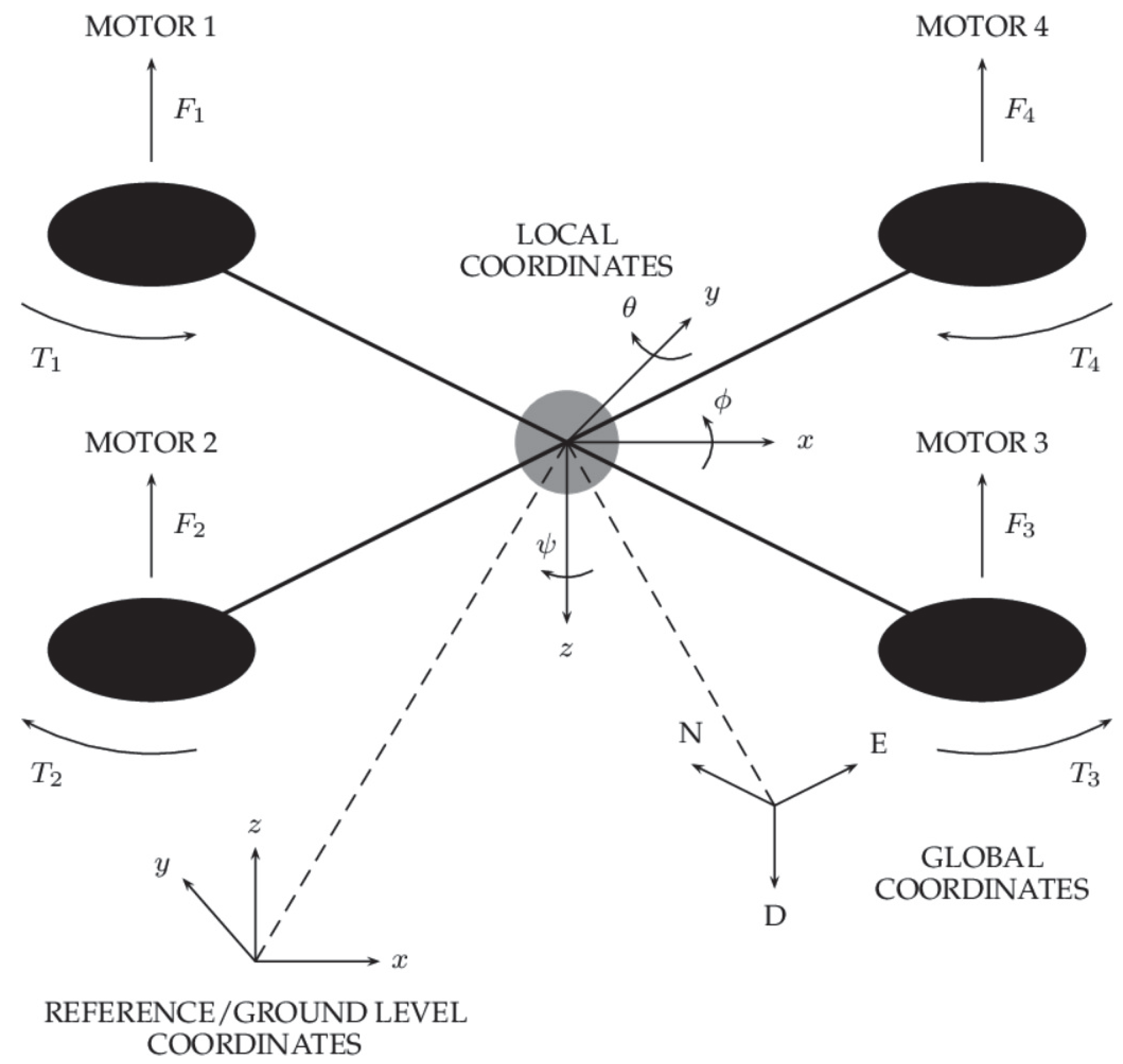
Let us describe a model of a Parrot Rolling Spider quadrotor driven by DC motors. In order to define position and orientation of this drone, global and local coordinate systems need to be introduced. The global system is described in NED convention (North-East-Down), and the local system has its origin in the geometrical center of the drone. Its axes, that is, x and y point towards the two adjacent motors, whereas the axis z points downwards. The orientation of the drone can be described using the Euler angles [13] as listed below. The coordinate system of a UAV and the Euler angles are depicted in Figure 1, with:

• $\varphi$ – angle w.r.t. the x axis (roll angle),
• $\theta$ – angle w.r.t. the y axis (pitch angle),
• $\psi$ – angle w.r.t. the z axis (yaw angle).

The transformation between global and local coordinates requires one to multiply three rotation matrices ${\mathit{R}}_{\mathrm{yaw}}$, ${\mathit{R}}_{\mathrm{pitch}}$ and ${\mathit{R}}_{\mathrm{roll}}$, respectively, to obtain the final transformation matrix ${\mathit{R}}_{\mathrm{W}2\mathrm{B}}$. In the transformations given below, the following notation has been adopted $s\left(\alpha \right):=sin\left(\alpha \right)$, $c\left(\alpha \right):=cos\left(\alpha \right)$, and:

$$\begin{array}{cc}{\mathit{R}}_{\mathrm{W}2\mathrm{B}}\hfill & ={\mathit{R}}_{\mathrm{yaw}}{\mathit{R}}_{\mathrm{pitch}}{\mathit{R}}_{\mathrm{roll}}=\hfill \\ \hfill & =\left[\begin{array}{ccc}c\left(\psi \right)& -s\left(\psi \right)& 0\\ s\left(\psi \right)& c\left(\psi \right)& 0\\ 0& 0& 1\end{array}\right]\left[\begin{array}{ccc}c\left(\theta \right)& 0& s\left(\theta \right)\\ 0& 1& 0\\ -s\left(\theta \right)& 0& c\left(\theta \right)\end{array}\right]\left[\begin{array}{ccc}1& 0& 0\\ 0& 1& -s\left(\varphi \right)\\ 0& s\left(\varphi \right)& c\left(\varphi \right)\end{array}\right]=\hfill \\ \hfill & =\left[\begin{array}{ccc}c\left(\theta \right)c\left(\psi \right)& c\left(\psi \right)s\left(\theta \right)s\left(\varphi \right)-c\left(\theta \right)s\left(\psi \right)& s\left(\varphi \right)s\left(\psi \right)+c\left(\varphi \right)c\left(\psi \right)s\left(\theta \right)\\ c\left(\theta \right)s\left(\psi \right)& c\left(\varphi \right)c\left(\psi \right)+s\left(\theta \right)s\left(\varphi \right)s\left(\psi \right)& c\left(\varphi \right)s\left(\theta \right)s\left(\psi \right)-c\left(\psi \right)s\left(\varphi \right)\\ -s\left(\theta \right)& c\left(\theta \right)s\left(\varphi \right)& c\left(\theta \right)c\left(\varphi \right)\end{array}\right].\hfill \end{array}$$

(1)

The backward transformation from local to global coordinates requires the matrix ${\mathit{R}}_{\mathrm{W}2\mathrm{B}}$ to be inverted,

$$\begin{array}{cc}{\mathit{R}}_{\mathrm{B}2\mathrm{W}}\hfill & ={\mathit{R}}_{\mathrm{W}2\mathrm{B}}^{-1}=\hfill \\ \hfill & =\left[\begin{array}{ccc}c\left(\theta \right)c\left(\psi \right)& c\left(\theta \right)s\left(\varphi \right)& -s\left(\theta \right)\\ c\left(\psi \right)s\left(\theta \right)s\left(\varphi \right)-c\left(\varphi \right)s\left(\psi \right)& c\left(\varphi \right)c\left(\psi \right)+s\left(\theta \right)s\left(\varphi \right)s\left(\psi \right)& c\left(\theta \right)s\left(\varphi \right)\\ s\left(\psi \right)s\left(\varphi \right)+c\left(\psi \right)c\left(\varphi \right)s\left(\theta \right)& c\left(\varphi \right)s\left(\psi \right)s\left(\theta \right)-c\left(\psi \right)s\left(\varphi \right)& c\left(\theta \right)c\left(\varphi \right)\end{array}\right].\hfill \end{array}$$

(2)

Similarly, the transformation from local rotational speeds $\underline{\mathsf{\Omega }}={[p,q,r]}^T$ to Euler angle derivatives $\underline{\dot{\mathsf{\Theta }}}={[\dot{\varphi },\dot{\theta },\dot{\psi }]}^T$ is possible when the inverse of Wronskian matrix $\mathit{W}$ is used [13]:

$$\begin{array}{cc}\underline{\dot{\mathsf{\Theta }}}\hfill & ={\mathit{W}}^{-1}\underline{\mathsf{\Omega }},\hfill \end{array}$$

(3)

$$\begin{array}{cc}{\mathit{W}}^{-1}\hfill & =\left[\begin{array}{ccc}c\left(\theta \right)& s\left(\varphi \right)s\left(\theta \right)& c\left(\varphi \right)s\left(\theta \right)\\ 0& c\left(\varphi \right)c\left(\theta \right)& -s\left(\varphi \right)c\left(\theta \right)\\ 0& s\left(\varphi \right)& c\left(\varphi \right)\end{array}\right].\hfill \end{array}$$

(4)

According to the second Newton’s principle, the acceleration exerted by the unbalanced force $\overrightarrow{F_w}$ on a body of a mass m is proportional to this force, and inversely proportional to its mass, that is,

$$\overrightarrow{F_w}=\frac{d}{dt}\left(m\overrightarrow{v}\right).$$

(5)

Having assumed that $\overrightarrow{F_w}=\overrightarrow{G}-\overrightarrow{T}$, where $\overrightarrow{G}$ is a gravity force vector, and $\overrightarrow{T}$ denotes the thrust vector generated by the propellers, Equation (5) can be extended to the form

$$\underline{\dot{v}}=\frac{1}{m}\left(\left[\begin{array}{c}0\\ 0\\ mg\end{array}\right]-{\mathit{R}}_{\mathrm{B}2\mathrm{W}}\left[\begin{array}{c}0\\ 0\\ T\end{array}\right]\right).$$

(6)

For the sake of brevity, the arrows above symbols will be henceforth omitted, as only numerical values will be considered. By substituting the matrix ${\mathit{R}}_{\mathrm{B}2\mathrm{W}}$ from Equation (2) to Equation (6), it is possible to obtain the acceleration vector in three axes of the local coordinate system of the UAV

$$\underline{\dot{v}}=\left[\begin{array}{c}\ddot{x}\\ \ddot{y}\\ \ddot{z}\end{array}\right]=\frac{1}{m}\left[\begin{array}{c}-T\left(c\right(\varphi \left)s\right(\theta \left)c\right(\psi )+s(\varphi \left)s\right(\psi \left)\right)\\ -T\left(c\right(\varphi \left)s\right(\theta \left)s\right(\psi )-s(\varphi \left)c\right(\psi \left)\right)\\ mg-T\left(c\right(\varphi \left)c\right(\theta \left)\right)\end{array}\right].$$

(7)

The thrust T generated by the propellers can be calculated on the basis of formulae below:

$$\begin{array}{cc}{T}_i\hfill & =K_a{\omega }_i^2,\hfill \end{array}$$

(8)

$$\begin{array}{cc}{K}_a\hfill & =C_t\rho \left(h\right)A{r}^2,\hfill \end{array}$$

(9)

$$\begin{array}{cc}T\hfill & =K_a\sum _{i=1}^n\left({\omega }_i^2\right),\hfill \end{array}$$

(10)

where:

• $T_i\left(\mathrm{N}\right)$ – thrust of the i–th propeller,
• $T\left(\mathrm{N}\right)$ – accumulated thrust of all propellers,
• ${\omega }_i\left(\frac{\mathrm{rad}}{\mathrm{s}}\right)$ – rotational speed of the i–th propeller,
• $K_a(\mathrm{kg}·\mathrm{m})$ – aerodynamical constant,
• $C_t$ – thrust constant,
• $\rho \left(\frac{\mathrm{kg}}{{\mathrm{m}}^3}\right)$ – air density,
• $h\left(\mathrm{m}\right)$ – propeller height,
• $A\left({\mathrm{m}}^2\right)$ – propeller area,
• $r\left(\mathrm{m}\right)$ – propeller radius,
• n – number of propellers.

The considered quadrotor ($n=4$) has six degrees of freedom, thus, in order to describe its state, 12 state variables are necessary [13],

$$\begin{array}{cc}\underline{x}\hfill & ={[{\mathrm{x}}_1,{\mathrm{x}}_2,{\mathrm{x}}_3,{\mathrm{x}}_4,{\mathrm{x}}_5,{\mathrm{x}}_6,{\mathrm{x}}_7,{\mathrm{x}}_8,{\mathrm{x}}_9,{\mathrm{x}}_{10},{\mathrm{x}}_{11},{\mathrm{x}}_{12}]}^T=\hfill \\ \hfill & ={[x,y,z,\varphi ,\theta ,\psi ,\dot{x},\dot{y},\dot{z},p,q,r]}^T.\hfill \end{array}$$

(11)

In Equation (11), the symbol $\underline{x}$ refers to a full state vector, whereas x and $\dot{x}$ are position and velocity of the UAV, respectively, in axis x, and so forth.

3. Model Reduction

The analysis of the landing process requires the model to be simplified. It is assumed that the UAV does not move in XY plane and keeps a horizontal alignment, thus without any loss of generality it can be assumed that:

$$\begin{array}{cc}x\hfill & =\dot{x}=\ddot{x}=y=\dot{y}=\ddot{y}=0,\hfill \end{array}$$

(12)

$$\begin{array}{cc}\varphi \hfill & =\theta =0.\hfill \end{array}$$

(13)

This assumption is realistic, and present in multiple pick-and-place tasks, as eventually, the control system of the UAV should keep this alignment. When environmental disturbances take place, the UAV is likely to be moved away from the landing position, but when emergency or planned landing is executed, the precision of landing in a spot is not of prime importance. It is a trajectory of descend the most important factor, thus the precise location of landing is not. Abiding Equations (12) and (13) strictly, would stipulate no exogenous disturbances occur. This simplification is somewhat naturel for tilt-hex constructions, see Reference [14] where the accumulative thrust force can be exerted in non-vertical direction, without tilting the structure, to compensate for the disturbances.

It has also been assumed that all four motors have the same rotational speed, leading to simplifying Equations (7) and (10) to the form of:

$$\begin{array}{cc}T\hfill & =4K_a{\omega }^2,\hfill \end{array}$$

(14)

$$\begin{array}{cc}\ddot{z}\hfill & =g-\frac{T}{m}=g-4\frac{K_a}{m}{\omega }^2.\hfill \end{array}$$

(15)

In order to enable any further analysis, the third coordinate system has been introduced, with the origin at the ground level, and the z axis pointing upwards. As the landing takes place while the altitude is not extremally high, it has been assumed that the air density does not vary, then:

$$\begin{array}{cc}\rho \hfill & =\mathrm{const}\Rightarrow K_a=\mathrm{const}.\hfill \end{array}$$

(16)

The symbolic expressions $\alpha$ and u have been defined as (:=):

$$\begin{array}{cc}\alpha :=\hfill & 4·\frac{K_a}{m},\hfill \end{array}$$

(17)

$$\begin{array}{cc}u:=\hfill & {\omega }^2,\hfill \end{array}$$

(18)

$$\begin{array}{cc}T\hfill & =\alpha u,\hfill \end{array}$$

(19)

$$\begin{array}{cc}\ddot{z}\hfill & =\alpha u-g,\hfill \end{array}$$

(20)

leading to the introduction of a simplified model of dynamics in the z axis

$${\dot{x}}_1=\ddot{z}=\alpha u-g$$

(21)

$${\dot{x}}_2=\dot{z}=x_1$$

(22)

in the third coordinate system, with the output equation (state-space equations) $y=x_2$.

The dynamical model of the UAV can be put in a matrix form (with the time indices omitted for brevity)

$$\begin{array}{cc}\underline{\dot{x}}\hfill & =\mathit{A}\underline{x}+\mathit{B}\underline{u},\hfill \end{array}$$

(23)

$$\begin{array}{cc}\left[\begin{array}{c}{\dot{x}}_1\\ {\dot{x}}_2\end{array}\right]\hfill & =\left[\begin{array}{cc}0& 0\\ 1& 0\end{array}\right]\left[\begin{array}{c}{x}_1\\ x_2\end{array}\right]+\left[\begin{array}{cc}\alpha & -1\\ 0& 0\end{array}\right]\left[\begin{array}{c}u\\ g\end{array}\right]\hfill \end{array}$$

(24)

with the output equation

$$y={\underline{c}}^T\underline{x}=[0,1]\underline{x}=x_2.$$

As can be seen, it is a typical case of a system which is structurally unstable (as $g\ne 0$ at all times), resembling many other dynamical structures, as a bicycle robot, subject to the same force, see Reference [15].

4. Landing Issues

The landing procedure is different from any control task of the UAV during the main phase of flight. The major difference is that reducing the current altitude to the ground level accepts no overshoots, which are typical in any transient processes during regulation tasks. The other issue is that different landing scenarios should be taken into consideration, as the UAV might undergo emergency landing or might land in a planned way. The first one can be given rise due to, for example, low battery levels or due to environmental issues. All the cases imply the landing trajectory $h_{\mathrm{start}}\to h_{\mathrm{ground}}$, to vary, where $h_{\mathrm{start}}$ denotes the initial altitude of the UAV at the time instant $t_0$, and $h_{\mathrm{ground}}$ denotes the ground level.

The following have been henceforth assumed:

$$\begin{array}{cc}z\left(0\right)\hfill & =h_{\mathrm{start}},\hfill \end{array}$$

(25)

$$\begin{array}{cc}z\left(t_f\right)\hfill & =\dot{z}\left(0\right)=\dot{z}\left(t_f\right)=0,\hfill \end{array}$$

(26)

$$\begin{array}{cc}z\left(t\right)\hfill & \ge 0,\hfill \end{array}$$

(27)

where $z\left(t\right)$ denotes the position of the UAV in z axis in the third coordinate system.

Among the others, it is important to classify landing procedures in the following pattern:

• minimum-time landing,
• minimum-energy landing,
• velocity-penalized landing,

as they arise from typical and emergency scenarios which can be potentially considered.

It is to be stressed that the generated reference trajectories should, in principle, be further fed to the altitude control loop to preserve desired behaviour of the UAV.

5. Minimum-Time Landing

The first scenario considered is the landing in the minimum time, which requires the optimization techniques to be adopted, and is connected to the following cost function:

$$J=\underset{0}{\overset{t_f}{\int }}\left(1\right)dt=t_f,$$

(28)

where $t_f$ is the duration of the landing procedure (final time), with the assumption that the thrust can be generated upwards only, and the propellers have a limited rotational speed

$$0\le u\le u_{\max }.$$

(29)

Following a standard routine for minimum-time problems, the following need to be calculated: ${\mathit{G}}_i=[{\underline{b}}_i,\mathit{A}{\underline{b}}_i,{\mathit{A}}^2{\underline{b}}_i,\dots ,{\mathit{A}}^{n-1}{\underline{b}}_i]:$

$$\begin{array}{cc}{\mathit{G}}_1\hfill & =\left[\begin{array}{cc}\left[\begin{array}{c}\alpha \\ 0\end{array}\right]& \left[\begin{array}{cc}0& 0\\ 1& 0\end{array}\right]\left[\begin{array}{c}\alpha \\ 0\end{array}\right]\end{array}\right]=\left[\begin{array}{cc}\alpha & 0\\ 0& \alpha \end{array}\right],\hfill \end{array}$$

(30)

$$\begin{array}{cc}{\mathit{G}}_2\hfill & =\left[\begin{array}{cc}\left[\begin{array}{c}-1\\ 0\end{array}\right]& \left[\begin{array}{cc}0& 0\\ 1& 0\end{array}\right]\left[\begin{array}{c}-1\\ 0\end{array}\right]\end{array}\right]=\left[\begin{array}{cc}-1& 0\\ 0& -1\end{array}\right],\hfill \end{array}$$

(31)

$$\begin{array}{cc}det\left({\mathit{G}}_1\right)\hfill & ={\alpha }^2,\hfill \end{array}$$

(32)

$$\begin{array}{cc}det\left({\mathit{G}}_2\right)\hfill & =1.\hfill \end{array}$$

(33)

to verify that the determinants of ${\mathit{G}}_1,{\mathit{G}}_2$ are non zero for $\alpha \ne 0$, and whether the minimum-time control is unique [16]. As known, such a scenario leads to a two-phase control: free falling phase, and braking phase with maximal $u=u_{\max }$ [16]. This is a common solution to minimum-time problems arising in control engineering practice, using for example, the minimum principle. The minimum-time control combined of two phases, makes use of the properties of the system, to allow maximum acceleration increase with no energy lost on rotating the propellers (motors stop), and the braking stage. In this sense, it resembles other approaches identified in the field, to use internal system properties to carry on control tasks, see Reference [17]. Below, $t_s$ denotes the switching time, $t_f$  is the grounding time, and $T_{\max }=\alpha u_{\max }$.

$$\begin{array}{c}\mathrm{First}\mathrm{landing}\mathrm{phase}:\hfill \\ \left\{\begin{array}{cc}u\hfill & =0\hfill \\ {\dot{x}}_1\hfill & =-g\hfill \end{array}\right.\hfill \end{array}\begin{array}{c}\mathrm{Sec}\mathrm{ond}\mathrm{landing}\mathrm{phase}:\hfill \\ \left\{\begin{array}{cc}u\hfill & =T_{\max }\hfill \\ {\dot{x}}_1\hfill & =T_{\max }-g\hfill \end{array}\right.\hfill \end{array}$$

$$\begin{array}{cc}\hfill x_1\left(0\right)=x_1\left(t_f\right)=0& \Rightarrow \underset{0}{\overset{t_s}{\int }}(-g)dt+\underset{t_s}{\overset{t_f}{\int }}(T_{\max }-g)dt=0,\hfill \\ \hfill 0& =-g{t}_s+(T_{\max }-g)(t_f-t_s),\hfill \\ \hfill g{t}_s& =(T_{\max }-g)t_f-(T_{\max }-g)t_s,\hfill \end{array}$$

$$\begin{array}{cc}\hfill T_{\max }{t}_s& =(T_{\max }-g)t_f,\hfill \\ \hfill t_f& =\frac{T_{\max }}{(T_{\max }-g)}{t}_s,\hfill \\ \hfill \gamma & =\frac{T_{\max }}{(T_{\max }-g)},\hfill \\ \hfill t_f& =\gamma t_s.\hfill \end{array}$$

Having assumed that assumptions Equations (25) and (26) hold and $\dot{z}\left(t_s\right)=-g{t}_s$, the velocity at the first phase of the landing procedure satisfies:

$$\begin{array}{cc}\hfill 0& =h_{\mathrm{start}}+\underset{0}{\overset{t_s}{\int }}(-gt)dt+\underset{0}{\overset{t_s}{\int }}\left(\dot{z}\left(0\right)\right)dt+\underset{t_s}{\overset{t_f}{\int }}\left((T_{\max }-g)t\right)dt+\underset{t_s}{\overset{t_f}{\int }}\left(\dot{z}\left(t_s\right)\right)dt,\hfill \\ \hfill 0& =h_{\mathrm{start}}-\frac{1}{2}g{t_s}^2+\frac{1}{2}(T_{\max }-g){(t_f-t_s)}^2+\dot{z}\left(t_s\right)(t_f-t_s),\hfill \\ \hfill -h_{\mathrm{start}}& =-\frac{1}{2}g{t_s}^2-\frac{1}{2}(g-T_{\max }){(t_f-t_s)}^2-g{t}_s(t_f-t_s),\hfill \\ \hfill h_{\mathrm{start}}& =\frac{1}{2}g{t_s}^2+\frac{1}{2}(g-T_{\max }){(t_f-t_s)}^2+g{t}_s(t_f-t_s),\hfill \\ \hfill h_{\mathrm{start}}& =\frac{1}{2}\left[(g-T_{\max }){(\gamma -1)}^2+g(2\gamma -1)\right]{t_s}^2,\hfill \\ \hfill h_{\mathrm{start}}& =\frac{1}{2}\left[(g-T_{\max }){\gamma }^2+2T_{\max }\gamma -T_{\max }\right]{t_s}^2,\hfill \end{array}$$

and for $\zeta :=\frac{1}{2}\left[(g-T_{\max }){\gamma }^2+2T_{\max }\gamma -T_{\max }\right]$:

$$\begin{array}{cc}\hfill h_{\mathrm{start}}& =\zeta {t_s}^2,\hfill \\ \hfill \zeta & =\frac{1}{2}\left[(g-T_{\max }){\gamma }^2+2T_{\max }\gamma -T_{\max }\right],\hfill \\ \hfill \zeta & =\frac{1}{2}\left[-(T_{\max }-g)\frac{T^2}{{(T_{\max }-g)}^2}+\frac{2{T_{\max }}^2}{(T_{\max }-g)}-\frac{T_{\max }(T_{\max }-g)}{(T_{\max }-g)}\right],\hfill \\ \hfill \zeta & =\frac{1}{2}\left[\frac{-{T_{\max }}^2+2T_{\max }^2-{T_{\max }}^2+g{T}_{max}}{(T_{\max }-g)}\right],\hfill \\ \hfill \zeta & =\frac{g{T}_{\max }}{2(T_{\max }-g)},\hfill \\ \hfill h_{\mathrm{start}}& =\zeta {t_s}^2\Rightarrow t_s=\sqrt{\frac{h_{\mathrm{start}}}{\zeta }}.\hfill \end{array}$$

The switching $t_s$ and grounding $t_f$ times satisfy:

$$\begin{array}{cc}{t}_s\hfill & =\sqrt{\frac{2h_{\mathrm{start}}(T_{\max }-g)}{g{T}_{\max }}},\hfill \end{array}$$

(34)

$$\begin{array}{cc}{t}_f\hfill & =\frac{T_{\max }}{(T_{\max }-g)}{t}_s,\hfill \end{array}$$

(35)

$$\begin{array}{cc}{t}_f\hfill & =\sqrt{\frac{2h_{\mathrm{start}}{T}_{\max }}{g(T_{\max }-g)}}.\hfill \end{array}$$

(36)

On the basis of Equations (34) and (36), it is possible to provide the analytical formula for the landing trajectory

$$\begin{array}{c}z\left(t\right)=x_2^{*}\left(t\right)=\left\{\begin{array}{ccc}{h}_{\mathrm{start}}-\frac{1}{2}g{t}^2\hfill & \iff & 0\le t<t_s\hfill \\ h_{\mathrm{start}}-\frac{1}{2}g{t_s}^2-g{t}_s(t-t_s)+\frac{1}{2}(T_{\max }-g){(t-t_s)}^2\hfill & \iff & t_s\le t<t_f\hfill \\ 0\hfill & \iff & t\ge t_f\hfill \end{array}.\right.\hfill \end{array}$$

(37)

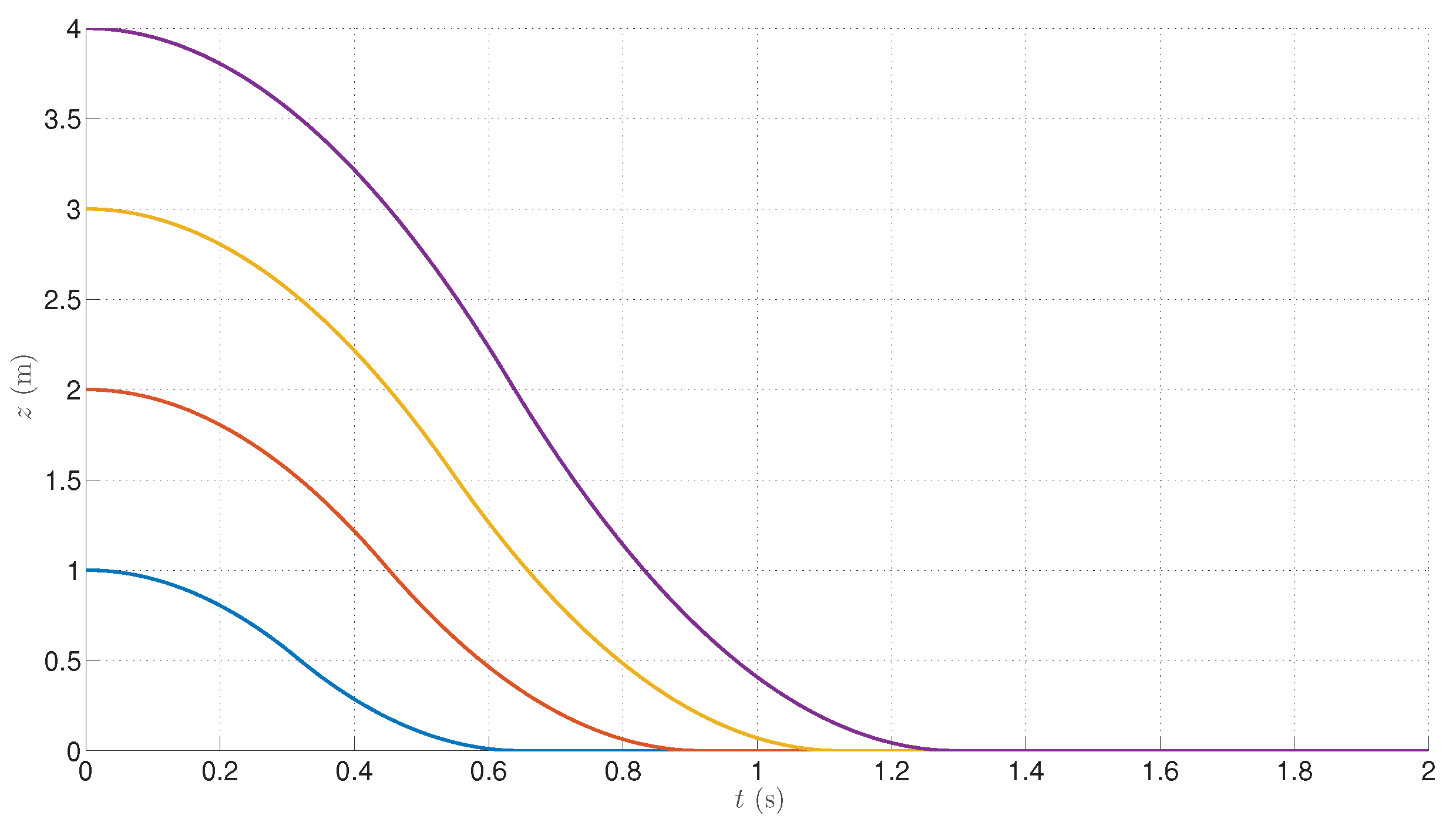
Sample landing trajectories for the Craig model have been presented in Figure 2 with the parameters of the Parrot Rolling Spider UAV and various initial altitudes:

$$\begin{array}{cc}\hfill C_t& =0.0107,\hfill \\ \hfill \rho & =1.184\frac{\mathrm{kg}}{{\mathrm{m}}^3},\hfill \\ \hfill r& =0.033\mathrm{m},\hfill \\ \hfill m& =0.068\mathrm{kg},\hfill \\ \hfill {\omega }_{\max }& =2630.67\frac{1}{\mathrm{s}}.\hfill \end{array}$$

6. Minimum-Energy Landing (False-zero Landing)

Minimum-energy landing is connected to the minimization of the performance index taking both altitude and control u effort (energy) into account, with the weight $\beta$ and

$$\begin{array}{cc}J\hfill & =\underset{0}{\overset{t}{\int }}\left(x_2+\beta u^2\right)dt,\hfill \end{array}$$

(38)

leading to the following optimization task:

$$\begin{array}{cc}\underset{u}{min}\hfill & J\hfill \end{array}$$

(39)

$$\begin{array}{cc}\mathrm{s}.\mathrm{t}.\hfill & {\dot{x}}_1=\alpha u-g\hfill \end{array}$$

(40)

$$\begin{array}{cc}\hfill & {\dot{x}}_2=x_1\hfill \end{array}$$

(41)

The task has been solved using the minimum principle of Pontryagin by minimizing the following Hamiltonian function [16,18]:

$$\begin{array}{cc}H\hfill & ={x_2}^2+\beta u^2+p_1(\alpha u-g)+p_2{x}_1.\hfill \end{array}$$

(42)

By transforming Equation (21) one gets:

$$\begin{array}{cc}\dot{x}\hfill & =\alpha u-g,\hfill \\ u\hfill & =\frac{1}{\alpha }(\dot{x_1}+g),\hfill \\ \dot{u}\hfill & =\frac{1}{\alpha }\ddot{x_1},\hfill \\ \ddot{u}\hfill & =\frac{1}{\alpha }{x_1}^{\left(3\right)}.\hfill \end{array}$$

Using the terminal condition $H^{*}\left(t\right)=H^{*}\left(t_f\right)=0$, and subject to no constraints imposed on $u\left(t\right)$:

$$\begin{array}{cc}\hfill \frac{\delta H}{\delta u}& =2\beta u+p_1\alpha =0,\hfill \\ \hfill p_1& =-\frac{2\beta }{\alpha }u,\hfill \\ \hfill \dot{p_1}& =-\frac{2\beta }{\alpha }\dot{u},\hfill \\ \hfill \ddot{p_1}& =-\frac{2\beta }{\alpha }\ddot{u},\hfill \\ \hfill \ddot{p_1}& =-\frac{2\beta }{\alpha }\frac{1}{\alpha }{x_1}^{\left(3\right)},\hfill \\ \hfill \ddot{p_1}& =-\frac{2\beta }{{\alpha }^2}{x_1}^{\left(3\right)},\hfill \end{array}$$

with:

$$\begin{array}{cc}\hfill \dot{p_1}& =-\frac{\delta H}{\delta x_1}=-p_2,\hfill \\ \hfill \dot{p_2}& =-\frac{\delta H}{\delta x_2}=-2x_2,\hfill \\ \hfill \ddot{p_1}& =2x_2,\hfill \\ \hfill 0& =\frac{\beta }{{\alpha }^2}{x_1}^{\left(3\right)}+x_2,\hfill \\ \hfill C& :=\frac{\beta }{{\alpha }^2},\hfill \\ \hfill 0& =C{x_1}^{\left(3\right)}+x_2|\frac{d}{dt},\hfill \\ \hfill 0& =C{x_1}^{\left(4\right)}+x_1,\hfill \end{array}$$

$$\begin{array}{cc}\hfill x_1& =e^{rt},\hfill \\ \hfill 0& =C{e^{rt}}^{\left(4\right)}+e^{rt},\hfill \\ \hfill 0& =C{r}^4{e}^{rt}+e^{rt}|:e^{rt},\hfill \\ \hfill 0& =C{r}^4+1,\hfill \\ \hfill \psi & :=\frac{\sqrt{2}}{2\sqrt[4]{C}},\hfill \\ \hfill r& =\left\{\begin{array}{c}\psi (1+j)\hfill \\ \psi (1-j)\hfill \\ -\psi (1+j)\hfill \\ -\psi (1-j).\hfill \end{array}\right.\hfill \end{array}$$

A general formula describing $x_1\left(t\right)$, $x_2\left(t\right)$ is given as:

$$\begin{array}{cc}{x}_1\left(t\right)=\hfill & e^{\psi t}(C_{1}c\left(\psi t\right)+C_{2}s\left(\psi t\right))+e^{-\psi t}(C_{3}c\left(\psi t\right)+C_{4}s\left(\psi t\right)),\hfill \\ x_2\left(t\right)=\hfill & \int (x_1\left(t\right))dt,\hfill \\ x_2\left(t\right)=\hfill & C_1\left(\frac{e^{\psi t}}{2{\psi }^2}(\psi c\left(\psi t\right)+\psi s\left(\psi t\right))\right)+C_2\left(\frac{e^{\psi t}}{2{\psi }^2}(\psi s\left(\psi t\right)-\psi c\left(\psi t\right))\right)+\hfill \\ & +C_3\left(\frac{e^{-\psi t}}{2{\psi }^2}(-\psi c\left(\psi t\right)+\psi s\left(\psi t\right))\right)+C_4\left(\frac{e^{-\psi t}}{2{\psi }^2}(-\psi s\left(\psi t\right)-\psi c\left(\psi t\right))\right),\hfill \\ x_2\left(t\right)=\hfill & \frac{1}{2\psi }\left[e^{\psi t}\left((C_1-C_2)c\left(\psi t\right)+(C_1+C_2)s\left(\psi t\right)\right)\right.+\hfill \\ & \left.+e^{-\psi t}\left((-C_3-C_4)c\left(\psi t\right)+(C_3-C_4)s\left(\psi t\right)\right)\right]+C_5.\hfill \end{array}$$

(43)

Using assumptions Equations (25) and (26), the integral constants can be found:

$$\begin{array}{c}\begin{array}{c}{x}_1\left(0\right)=0\Rightarrow C_1+C_3=0\hfill \\ x_1(t_f\to \infty )=0\Rightarrow C_1=C_2=0\hfill \end{array}\}\hspace{1em}\Rightarrow C_3=0\hfill \\ x_2(t_f\to \infty )=0\Rightarrow C_5=0,\hfill \\ x_2\left(0\right)=h_{\mathrm{start}},\hfill \\ h_{\mathrm{start}}=\frac{1}{2\psi }(-C_3-C_4)+C_5,\hfill \\ C_4=-2\psi h_{\mathrm{start}},\hfill \\ x_2\left(t\right)=h_{\mathrm{start}}{e}^{-\psi t}\left(c\right(\psi t)+s(\psi t\left)\right).\hfill \end{array}$$

(44)

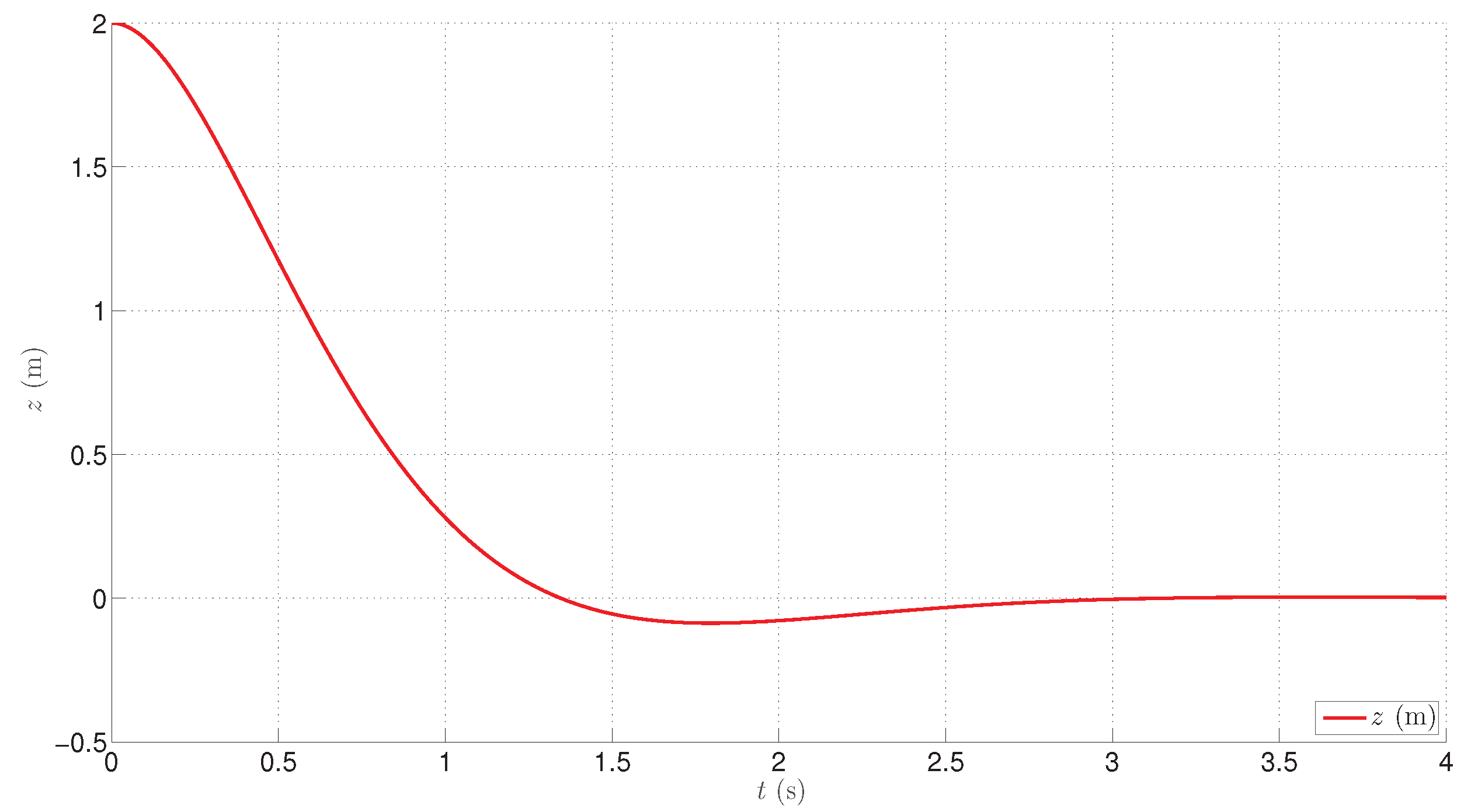
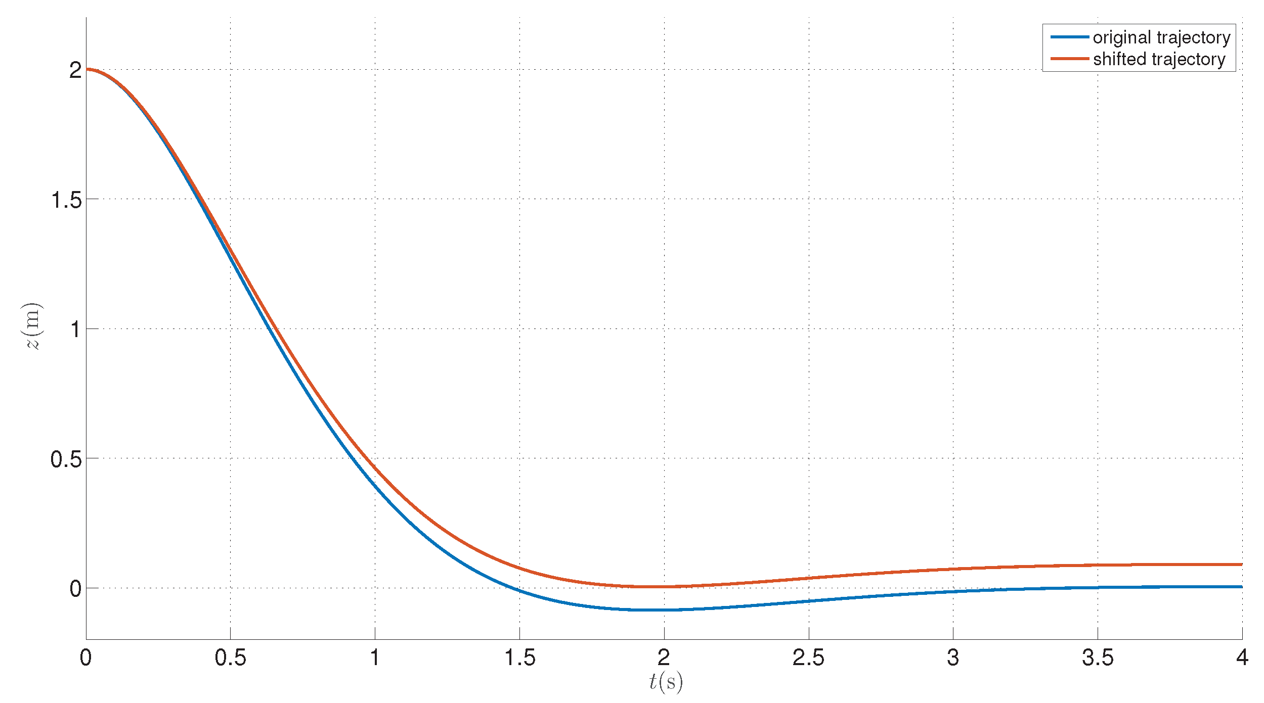
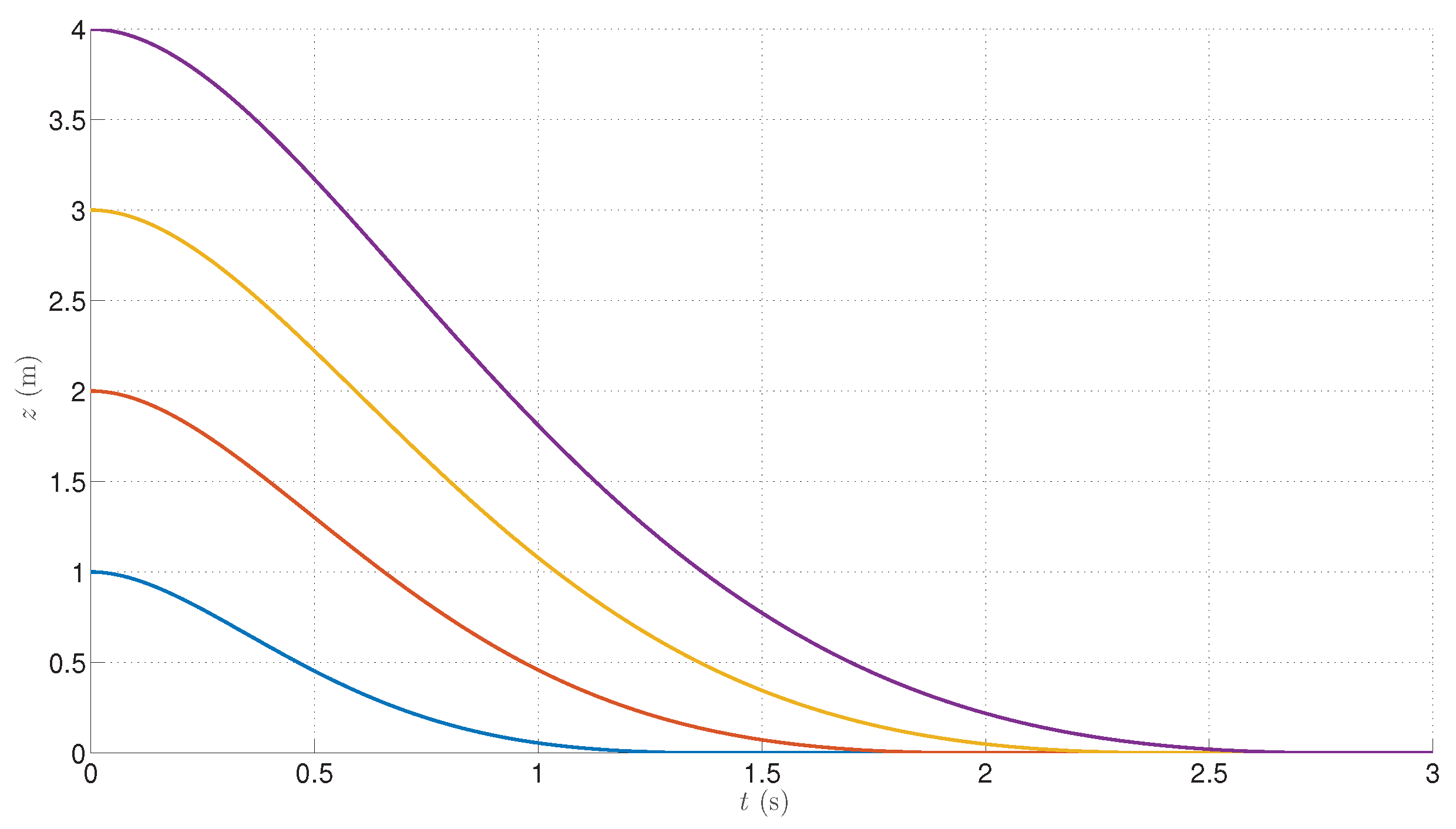
Finally, the formula describing trajectories depicted in Figure 3 has been obtained. As can be seen, the altitude while landing, falls below zero due to the overshoot phenomenon, what is not acceptable, though definitely shortens the regulation time (typical regulation time vs. damping ratio interplay). In order to compensate for the latter, it has been established that $x_2\left(t\right)$ reaches the ground level at $t=\frac{\pi }{\psi }$, and the landing phase can be splitted into two phases:

$$\begin{array}{cc}{x}_2\left(t\right)\hfill & =\left\{\begin{array}{cc}f\left(t\right)\hfill & \iff 0<t\le \frac{\pi }{\psi }\hfill \\ 0\hfill & \iff t>\frac{\pi }{\psi }\hfill \end{array}\right.,\hfill \end{array}$$

(45)

where $f\left(t\right)$ results from Equation (43) and reduces the altitude between $h_{\mathrm{start}}\to 0$. In order to eliminate the impact of the overshoot on the landing phase, the ground level should be virtually raised so that the minimum of Equation (43) equals always zero, what explains the ’false zero’ name of the approach. The latter has been shown in Figure 4.

The latter implies that the conditions Equations (25) and (26) must be satisfied at all times where:

$$\begin{array}{ccc}{x}_1\left(0\right)=0\hfill & x_1(\frac{\pi }{\psi })=0\hfill & x_1(t_f\to \infty )=0\hfill \\ x_2\left(0\right)=h_{\mathrm{start}}\hfill & x_2(\frac{\pi }{\psi })=0\hfill & x_2(t_f\to \infty )=h_e\hfill \end{array}.$$

(46)

From relations Equation (46) one gets:

$$\begin{array}{c}\begin{array}{c}{x}_1\left(0\right)=0\Rightarrow C_1+C_3=0\hfill \\ x_1(t_f\to \infty )=0\Rightarrow C_1=C_2=0\hfill \end{array}\}\hspace{1em}\Rightarrow C_3=0,\hfill \\ x_2(t_f\to \infty )=h_e\Rightarrow C_5=h_e,\hfill \\ x_2\left(0\right)=h_{\mathrm{start}}\Rightarrow h_{\mathrm{start}}=\frac{-C_4}{2\psi }+h_e,\hfill \\ C_4=-2\psi (h_{\mathrm{start}}-h_e),\hfill \\ x_2(\frac{\pi }{\psi })=0\Rightarrow 0=-\frac{e^{-\pi }}{2\psi }(-C_4)+h_e,\hfill \\ e^{-\pi }(h_{\mathrm{start}}-h_e)=h_e,\hfill \\ h_{\mathrm{start}}=h_e(1+e^{\pi }),\hfill \\ h_e=\frac{h_{\mathrm{start}}}{(1+e^{\pi })},\hfill \\ C_4=-2\psi h_{\mathrm{start}}(1-\frac{h_{\mathrm{start}}}{(1+e^{\pi })}),\hfill \\ x_2^{*}(t)=\{\begin{array}{cc}{h}_{start}\left(e^{-\psi t}(1-\frac{h_{\mathrm{start}}}{(1+e^{\pi })})(c\left(\psi t\right)+s\left(\psi t\right))+(1-\frac{h_{\mathrm{start}}}{(1+e^{\pi })})\right)\hfill & \iff 0<t\le \frac{\pi }{\psi }\hfill \\ 0\hfill & \iff t>\frac{\pi }{\psi }\hfill \end{array}\hfill \end{array}$$

(47)

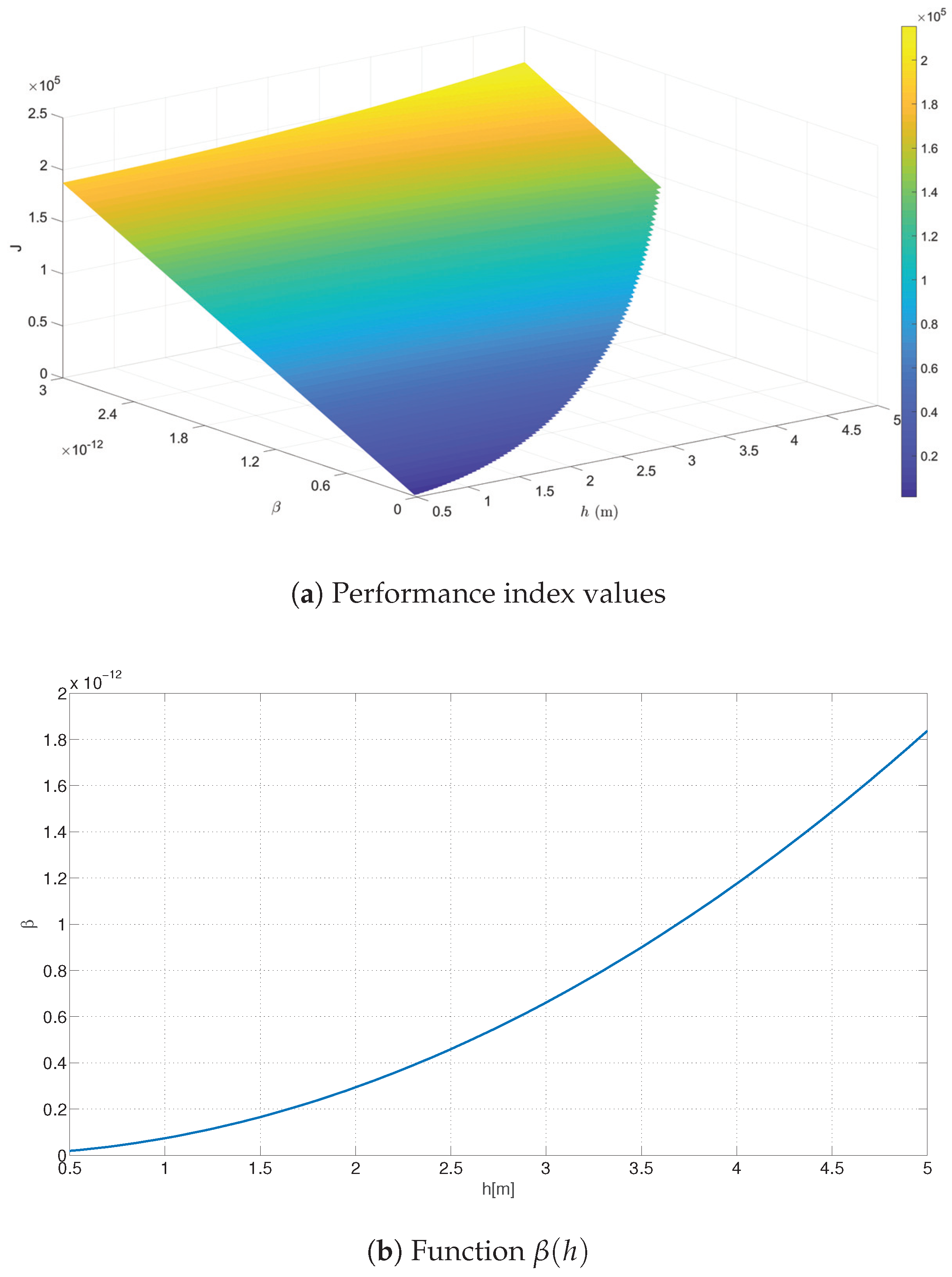
It is to be borne in mind that in order to use the trajectory evaluated, the correct value of $\beta$ must be stipulated first, and subsequently used in the performance index  Equation (38). The evaluation of this parameter can be done iteratively by creating, at first, two vectors, which: include a set of initial altitudes, say ranging between $0.5\mathrm{m}$ up to $5\mathrm{m}$ with the step of $0.05\mathrm{m}$, and the vector of 4000 equally-spaced samples of candidate $\beta$ values in the range of $〈0;3\times {10}^{-12}〉$. The choice of the final value of the parameter is based on evaluation of various trajectories for every pair of the above-mentioned parameters, according to relation Equation (38). Secondly, the samples with negative thrust force need to be removed, and finally, the value of $\beta$ is based on the minimal value of J for consecutive initial altitude. The results of such iterative calculations is presented in Figure 5.

The function implementing the calculations in Matlab has been presented in Appendix A (Algorithm A1).

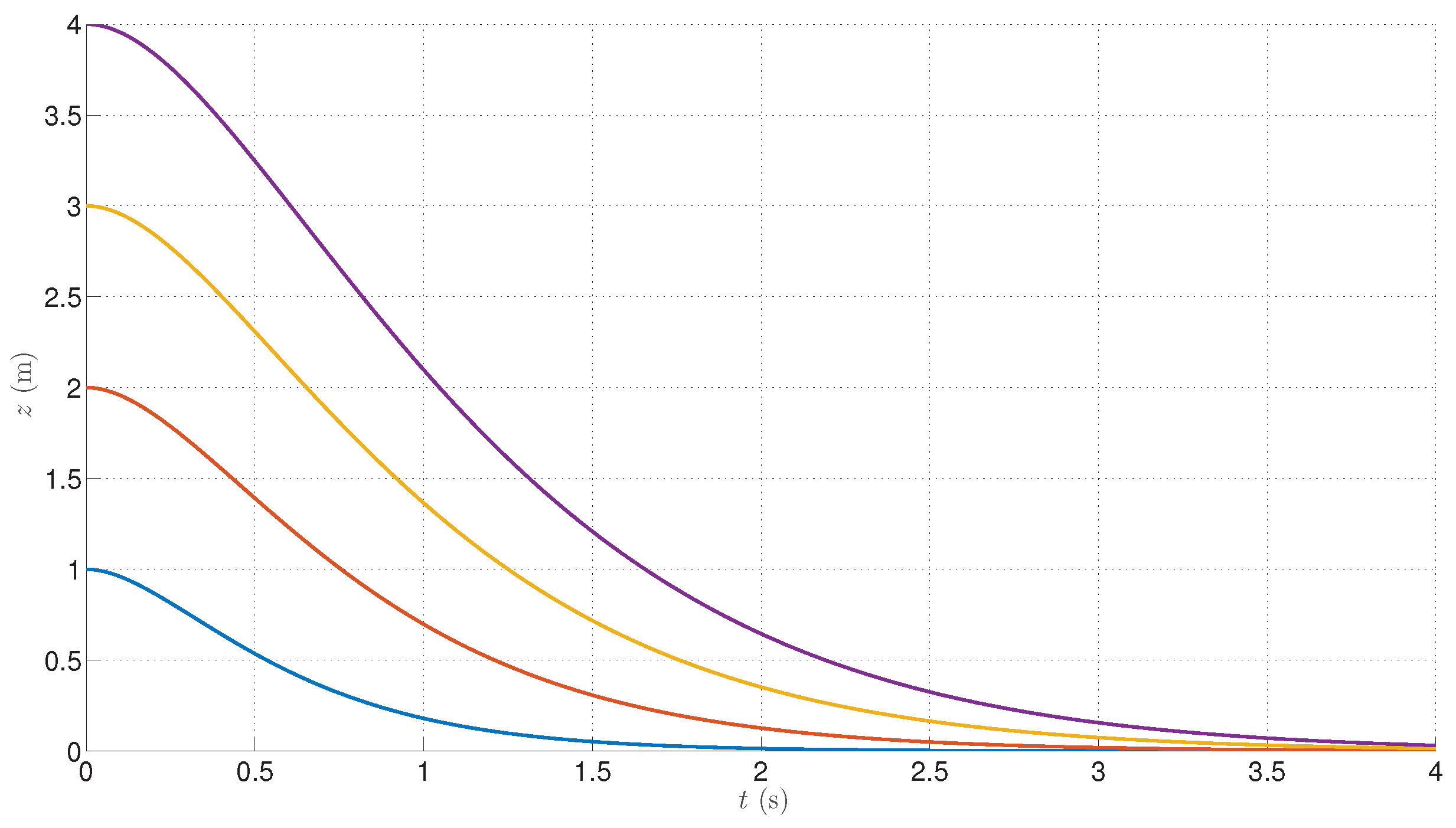
Once the final formula for the landing trajectory $x_2\left(t\right)$ is found, and accompanied by the optimal $\beta$, it is possible to calculate the trajectories for a specific test conditions. Sample trajectories have been presented in Figure 6.

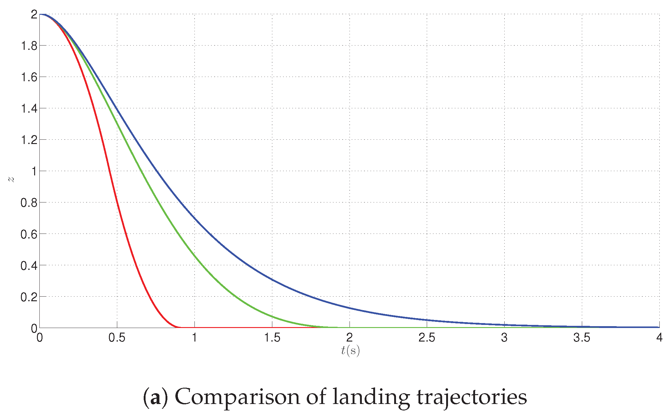
7. Velocity-Penalized Landing

The trajectories presented in Section 5 and Section 6 can be used during emergency landing, when either time or energy considerations are of prime importance. In these cases, the landing process is fast, and coupled with a huge jerk or snap. However, during the planned landing phase it is useful to take the performance index penalizing the velocity of a drone in the z axis and taking energy considerations into account. During the calculations, a variational calculus approach with constraints is adopted [16], and a penalty taking control signal energy is included into the performance index, to shorten the landing time,

$$J=\underset{0}{\overset{t}{\int }}({x_1}^2+\beta u^2)dt.$$

(48)

It is necessary to transform the cost function Equation (48) using Equations (21) and (22) into:

$$\begin{array}{cc}J\hfill & =\underset{0}{\overset{t}{\int }}\left({x_1}^2+\beta u^2\right)dt=\underset{0}{\overset{t}{\int }}\left({\dot{x}}_2{}^2+\beta {\left(\frac{{\dot{x}}_1}{\alpha }+\frac{g}{\alpha }\right)}^2\right)dt=\hfill \\ \hfill & =\underset{0}{\overset{t}{\int }}\left({\dot{x}}_2{}^2+\frac{\beta }{\alpha }{\left({\dot{x}}_1+g\right)}^2\right)dt.\hfill \end{array}$$

Having assumed that $\gamma :=\frac{\beta }{\alpha }$,

$$\begin{array}{cc}J\hfill & =\underset{0}{\overset{t}{\int }}\left({\dot{x}}_2{}^2+\gamma \left({\dot{x}}_1{}^2+2g{\dot{x}}_1+g^2\right)\right)dt=\hfill \\ \hfill & =\underset{0}{\overset{t}{\int }}\left({\dot{x}}_2{}^2+\gamma {\ddot{x}}_2{}^2+2g\gamma {\ddot{x}}_2+\gamma g^2\right)dt.\hfill \end{array}$$

(49)

In order to find the extremum of the functional Equation (49), it is necessary to satisfy the following Euler-Poisson equations for all the functions which are presented in Reference [18]:

$$\frac{\delta f}{\delta x_i}-\frac{d}{dt}\left(\frac{\delta f}{\delta {\dot{x}}_i}\right)+\frac{d^2}{d{t}^2}\left(\frac{\delta f}{\delta {\ddot{x}}_i}\right)-\cdots +{(-1)}^n\frac{d^n}{d{t}^n}\left(\frac{\delta f}{\delta x_i{}^{\left(n\right)}}\right)=0,$$

(50)

where $x_i{}^{\left(n\right)}$ stands for the n-th order derivative of $x_i$ with respect to time. Abiding standard Euler notation, the sub-derivative expressions take the following form: for $n=1$ one gets $\frac{\delta f}{\delta {\dot{x}}_i}$, for $n=2$, $\frac{\delta f}{\delta {\ddot{x}}_i}$, and so forth.

On the basis of the sub-integral function in Equation (49), a Lagrangean must be defined at first. The term $\gamma g^2$ has not been included in the performance index, as it is a constant value and has no impact on the precise localisation of the extremum of the functional. In addition, the Lagrange multiplier $\lambda$ is included into the formula and results from the assumption Equation (27) $x_2\ge 0\Rightarrow -x_2+{\kappa }^2=0$:

$$\begin{array}{cc}\hfill L(t,x_2,{\dot{x}}_2,{\ddot{x}}_2,\lambda ,\kappa )& ={\dot{x}}_2{}^2+\gamma {\ddot{x}}_2{}^2+2g\gamma {\ddot{x}}_2+\lambda (-x_2+\kappa ),\hfill \\ \hfill L& =0.\hfill \end{array}$$

(51)

In order to formulate the Euler-Poisson equation, it is necessary to calculate the following derivatives of L:

$$\begin{array}{cccc}\frac{\delta L}{x_2}\hfill & =-\lambda ,\hfill & & \\ \frac{\delta L}{{\dot{x}}_2}\hfill & =2{\dot{x}}_2,\hfill & \frac{d}{dt}\left(\frac{\delta L}{{\dot{x}}_2}\right)\hfill & =2{\ddot{x}}_2,\hfill \\ \frac{\delta L}{{\ddot{x}}_2}\hfill & =2\gamma g+2\gamma {\ddot{x}}_2,\hfill & \frac{d^2}{d{t}^2}\left(\frac{\delta L}{{\ddot{x}}_2}\right)\hfill & =2\gamma x_2{}^{\left(4\right)},\hfill \\ \frac{\delta L}{\delta \lambda }\hfill & =-x_2+{\kappa }^2,\hfill & \frac{d}{dt}\left(\frac{\delta L}{\lambda }\right)\hfill & =0,\hfill \\ \frac{\delta L}{\delta \kappa }\hfill & =2\lambda \kappa ,\hfill & \frac{d}{dt}\left(\frac{\delta L}{\kappa }\right)\hfill & =0.\hfill \end{array}$$

On the basis of the latter, and Equation (50), the final set the necessary conditions of optimality is formulated:

$$\begin{array}{c}\left\{\begin{array}{cc}0\hfill & =-\lambda -2{\ddot{x}}_2+2\gamma x_2{}^{\left(4\right)}\hfill \\ 0\hfill & =-x_2+{\kappa }^2\hfill \\ 0\hfill & =2\lambda \kappa \hfill \end{array}\right..\hfill \end{array}$$

(52)

Two cases need to be considered here, namely $\lambda \ne 0$ and $\lambda =0$:

$$\begin{array}{cc}\hfill & \underline{\mathrm{Case}\mathrm{I}}-\mathrm{constraint}\mathrm{Equation}\left(27\right)\mathrm{is}\mathrm{active}(\mathrm{z}=0):\hfill \\ \hfill & \left\{\begin{array}{cc}\lambda \hfill & \ne 0\hfill \\ \lambda \kappa \hfill & =0,\hfill \end{array}\right.\hfill \\ \hfill & \kappa =0,\hfill \\ \hfill & 0=-x_2+{\kappa }^2,\hfill \\ \hfill & x_2=0.\hfill \end{array}$$

(53)

$$\begin{array}{cc}\hfill & \underline{\mathrm{Case}\mathrm{II}}-\mathrm{constraint}\mathrm{Equation}\left(27\right)\mathrm{is}\mathrm{inactive}(\mathrm{z}>0):\hfill \\ \hfill & \left\{\begin{array}{cc}\lambda \hfill & =0\hfill \\ \lambda \kappa \hfill & =0\hfill \end{array}\right.\Rightarrow \left\{\begin{array}{c}\kappa \in \mathrm{\Re }\hfill \\ x_2\in 〈0,\infty 〉,\hfill \end{array}\right.\hfill \\ \hfill & 0=-2{\ddot{x}}_2+2\gamma x_2{}^{\left(4\right)},\hfill \\ \hfill & 0=\gamma {\ddot{x}}_2{}^{\left(4\right)}-{\ddot{x}}_2,\hfill \\ \hfill & x_2=e^{rt},\hfill \\ \hfill & 0=\gamma {\left(e^{rt}\right)}^{\left(4\right)}-{\left(e^{rt}\right)}^{\left(2\right)},\hfill \\ \hfill & 0=\gamma r^4-r^2,\hfill \\ \hfill & 0=r^2\left(\gamma r^2-1\right),\hfill \\ \hfill & \psi :=\sqrt{\frac{1}{\gamma }},\hfill \\ \hfill & x_2=C_{1}t+C_2+e^{-\psi t}\left(C_{3}c\left(\gamma t\right)+C_{4}s\left(\gamma t\right)\right).\hfill \end{array}$$

(54)

By using Equation (22), a time derivative of Equation (54) can be calculated:

$$\begin{array}{cc}\hfill & x_1=\frac{d}{dt}\left(x_2\right),\hfill \\ \hfill & x_1=C_1-\psi e^{-\psi t}\left(C_{3}c\left(\gamma t\right)+C_{4}s\left(\gamma t\right)\right)+e^{-\psi t}\left(-\gamma C_{3}s\left(\gamma t\right)+\gamma C_{4}c\left(\gamma t\right)\right),\hfill \end{array}$$

(55)

$$\begin{array}{c}\begin{array}{cc}{x}_1=C_1\hfill & +C_3{e}^{-\psi t}\left(-\psi c\left(\gamma t\right)-\gamma s\left(\gamma t\right)\right)+C_4{e}^{-\psi t}\left(-\psi s\left(\gamma t\right)+\gamma c\left(\gamma t\right)\right).\hfill \end{array}\hfill \end{array}$$

(56)

On the basis of the expressions from Equations (25), (26), (54) and (56), the integral constants $C_{1÷4}$ can be obtained:

$$\begin{array}{c}\begin{array}{c}{x}_1\left(0\right)=0\Rightarrow C_1+C_3(-\psi )+C_4\gamma =0\hfill \\ x_1(t_f\to \infty )=0\Rightarrow C_1=0\hfill \end{array}\}\hspace{1em}\Rightarrow C_4=\frac{\psi }{\gamma }{C}_3,\hfill \\ \begin{array}{c}{x}_2\left(0\right)=h_{\mathrm{start}}\Rightarrow C_2+C_3=h_{\mathrm{start}}\hfill \\ x_2(t_f\to \infty )=0\Rightarrow C_2=0\hfill \end{array}\}\hspace{1em}\Rightarrow C_3=h_{\mathrm{start}},\hfill \\ C_4=\frac{\psi }{\gamma }{h}_{\mathrm{start}},\hfill \\ x_1^{*}(t)=h_{\mathrm{start}}(e^{-\psi t}(-\psi c(\gamma t)-\gamma s(\gamma t))+\frac{\psi }{\gamma }{e}^{-\psi t}(-\psi s(\gamma t)+\gamma c(\gamma t))),\hfill \end{array}$$

(57)

$$x_2^{*}(t)=h_{\mathrm{start}}{e}^{-\psi t}(c(\gamma t)+\frac{\psi }{\gamma }s(\gamma t)).$$

(58)

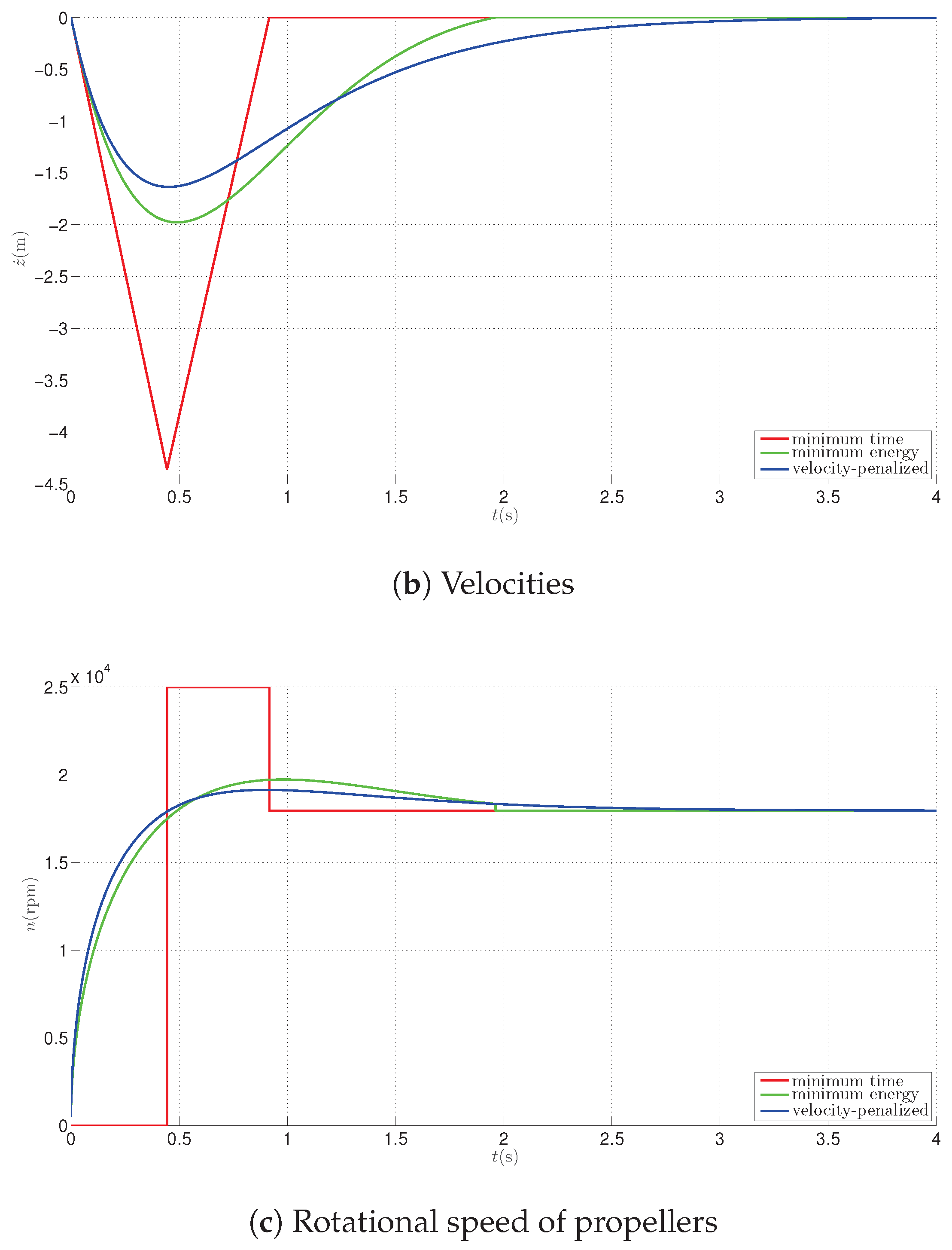
As in the case of minimum-energy landing, $\beta$ should also be optimized using, preferably, the same method, though in this case $\beta \in 〈0;2\times {10}^{-6}〉$, and the cost function takes the form of Equation (48). The listing of a function implementing this idea is given in Appendix A (Algorithm A1). Figure 7 presents velocity-penalized landing trajectories for various initial altitudes.

8. Comparison of the Obtained Trajectories

The trajectories obtained in Section 5, Section 6 and Section 7 have been presented in Figure 8. As can be seen, the time of the landing phase and velocities differ as the function of the selected landing scenario. Having assumed that landing is terminated whenever the difference between the ground level and the current altitude does not exceed $0.01\mathrm{m}$, the results have been given in

Table 1. Comparison of trajectories.

Trajectory	Landing Time to $\mathit{z}<0.01\mathbf{m}\left(\mathbf{s}\right)$	Minimal Altitude $\left(\mathbf{m}\right)$
Minimum-time	$0.871$	$4.4409\times {10}^{-17}$
Minimum-energy	$1.768$	$5.4839\times {10}^{-9}$
Velocity-penalized	$3.317$	$2.5135\times {10}^{-3}$

. The value $0.01\mathrm{m}$ is arbitrary, and is reflected by the way the real Rolling Spider UAV is affected by disturbances, resulting from the air flow, and poor precision of its inertial measurement unit (IMU).

The methodology behind selecting the gain for the integral term in the PID controller is depicted in Figure 9. By comparing the experiments for various values of the I term gain, the value of 0.01 was selected to mimic relatively fast response time in hover state, while keeping good damping ratio of the control loop. It is a common practice in UAV that controllers actually act like PD controllers, when the I term has low gains.

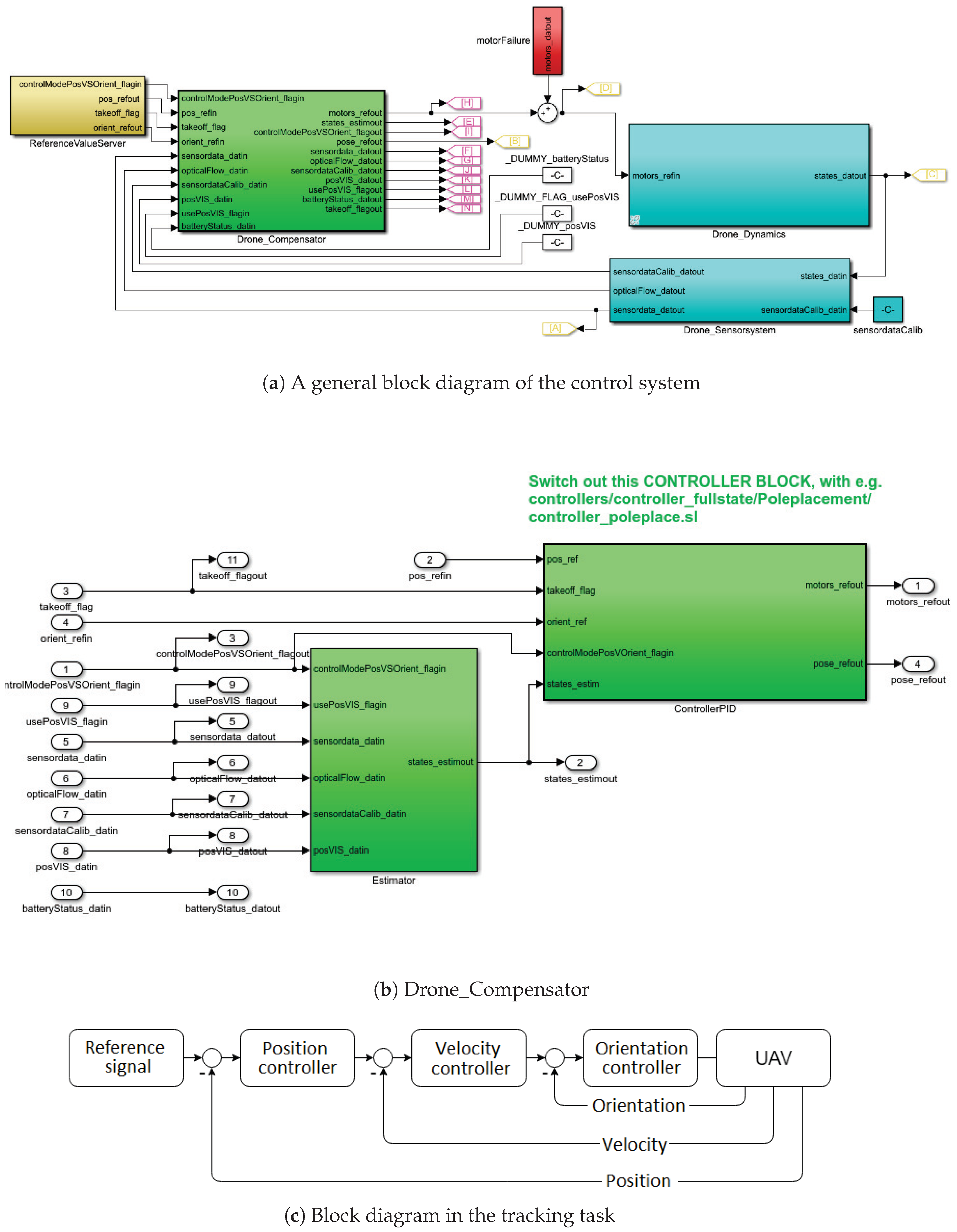
9. Simulink Support Package for Parrot Minidrones

By using the Simulink Support Package for Parrot Minidrones in Matlab is was possible to simulate the behaviour of the drone in safe conditions, and to verify the obtained optimization results. The software enables one to obtain access to all the signals that would be available from the real machine, with the block diagram in the Simulink given in Figure 10.

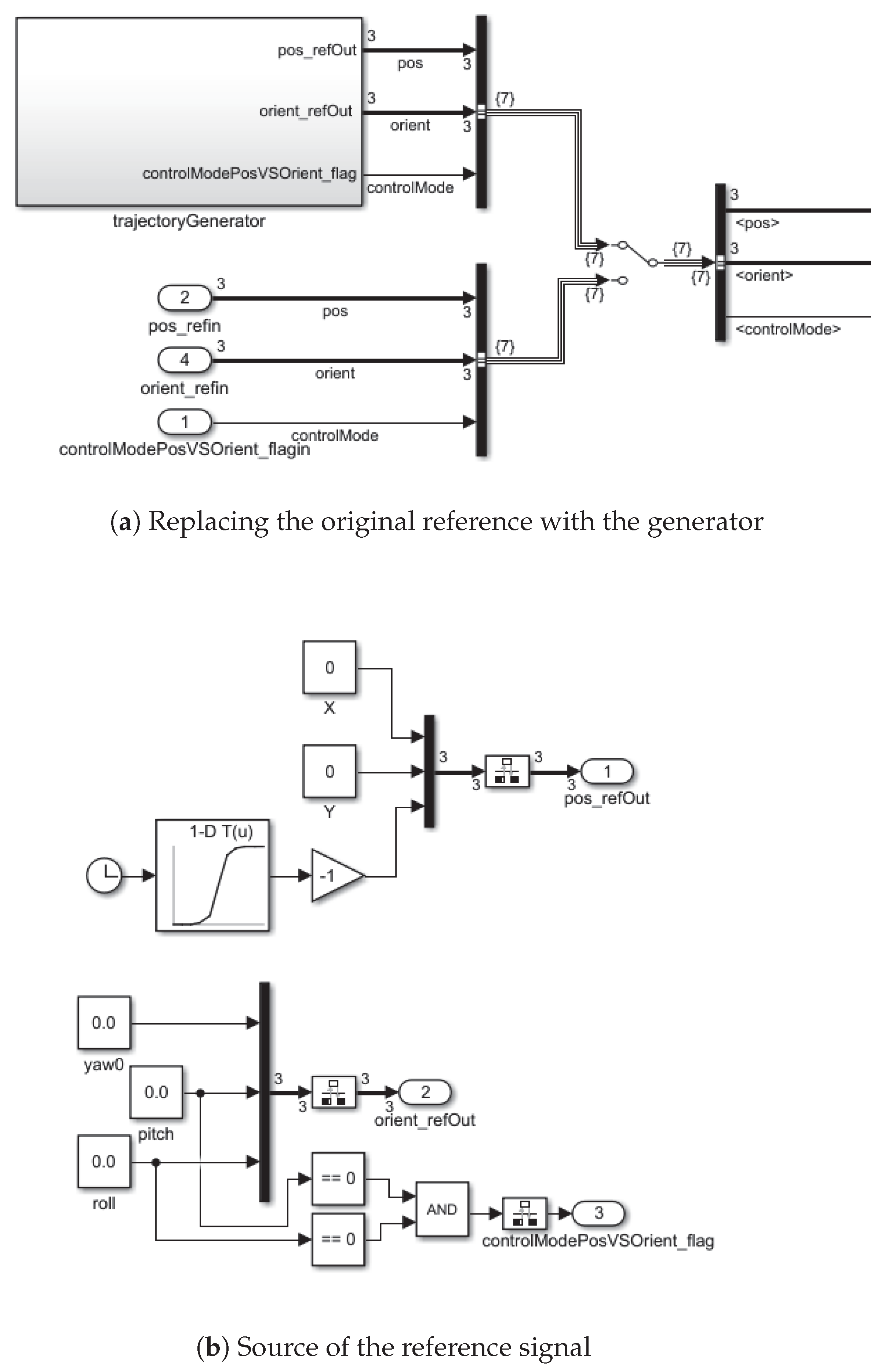
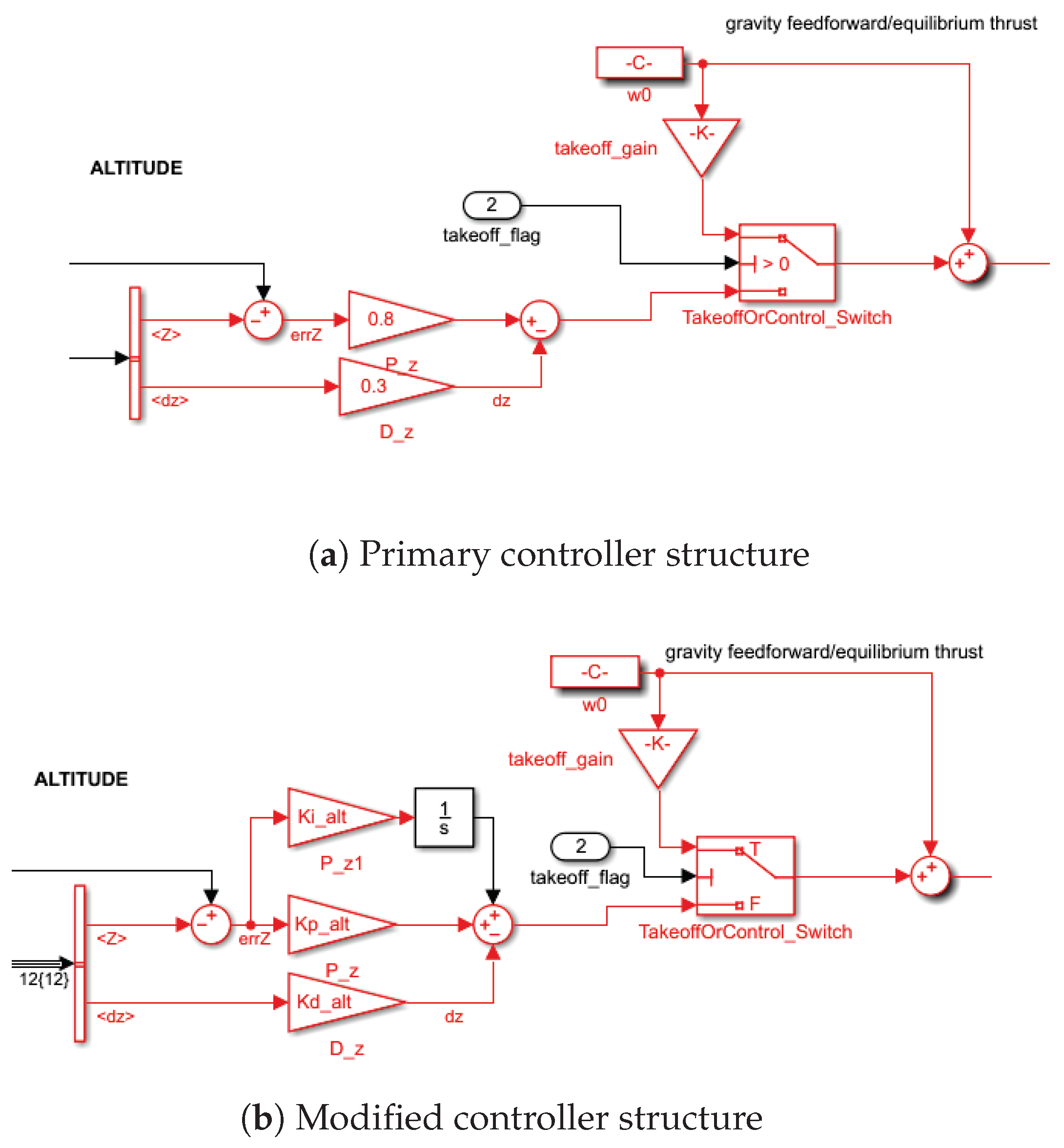
The basic block diagram has been modified so that it is possible to provide the reference trajectory, see Figure 11. Its block diagram depicted using standard control blocks, is presented in Figure 10c. The position signal is connected here to the altitude component which is fed back from the estimator, see Reference [19]. This model, as well as many other mathematical models have been made available to the public by Mathematical Model Database, see Reference [20]. As the Simulink model is implemented in NED convention, the sign of the z coordinate in the Simulink block diagram has to be changed to the opposite.

The control system provided by the developer contains the altitude, XY position, yaw, roll and pitch controllers. According to Equation (7) the translation in z axis in independent from the movement in the horizontal plane, thus the modification of the altitude controller is possible without any changes in the remaining controllers.

In order to eliminate the steady-state error, an integral action has been added to the original PD controller, with the integral gain set as $K_I=0.01$, see Figure 12, where the controller is given by ($e\left(t\right)=z_{\mathrm{ref}}\left(t\right)-z\left(t\right)$, as the tracking error, and $z_{\mathrm{ref}}\left(t\right)$ as the reference signal),

$$\begin{array}{cc}u\left(t\right)\hfill & =k_{P}e\left(t\right)+k_D\frac{de}{dt},\hfill \end{array}$$

(59)

$$\begin{array}{cc}u\left(t\right)\hfill & =k_{P}e\left(t\right)+k_I\int e\left(t\right)dt+k_D\frac{de}{dt}.\hfill \end{array}$$

(60)

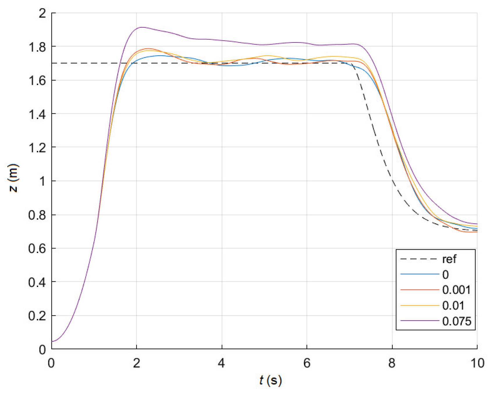
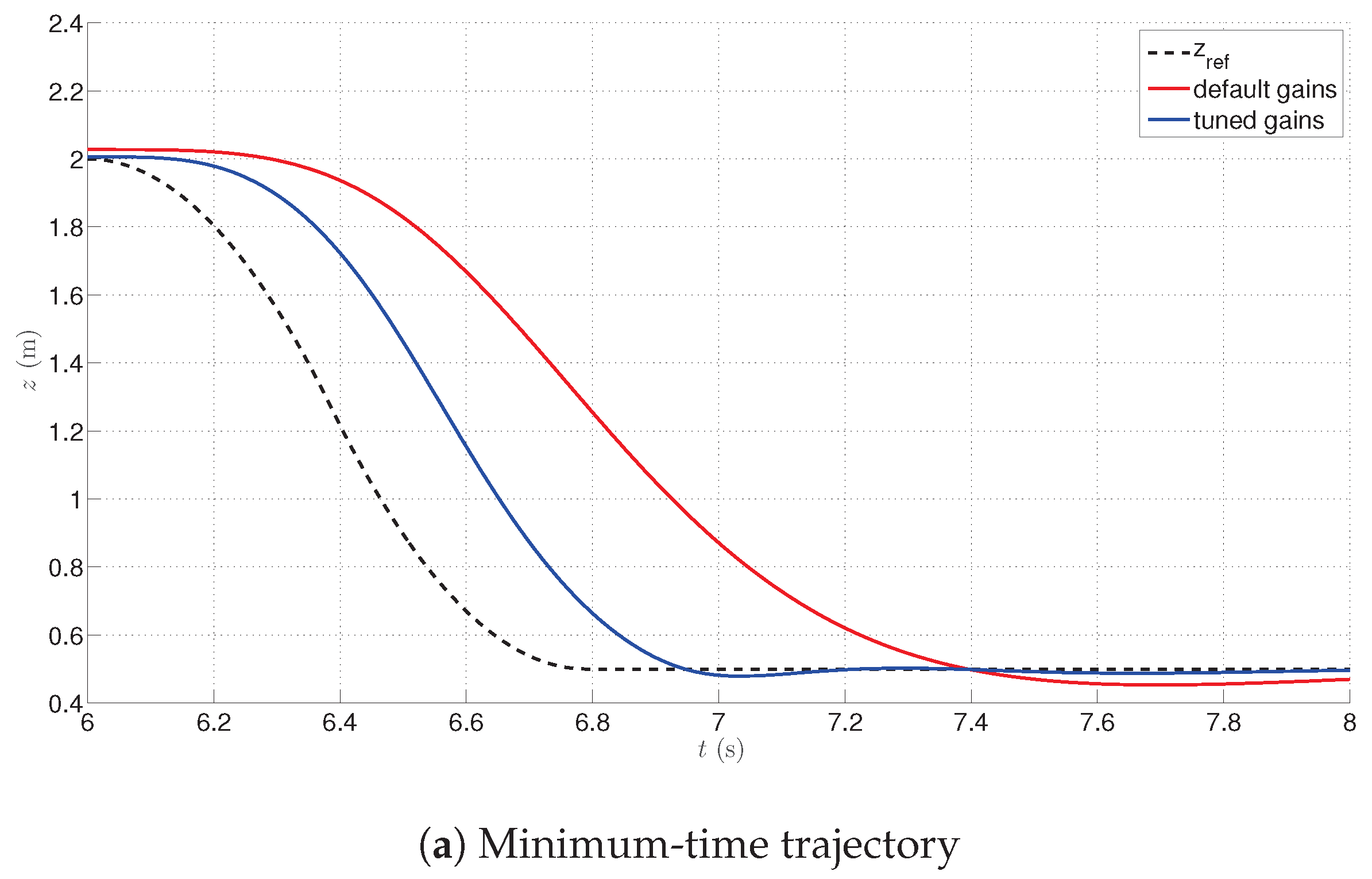
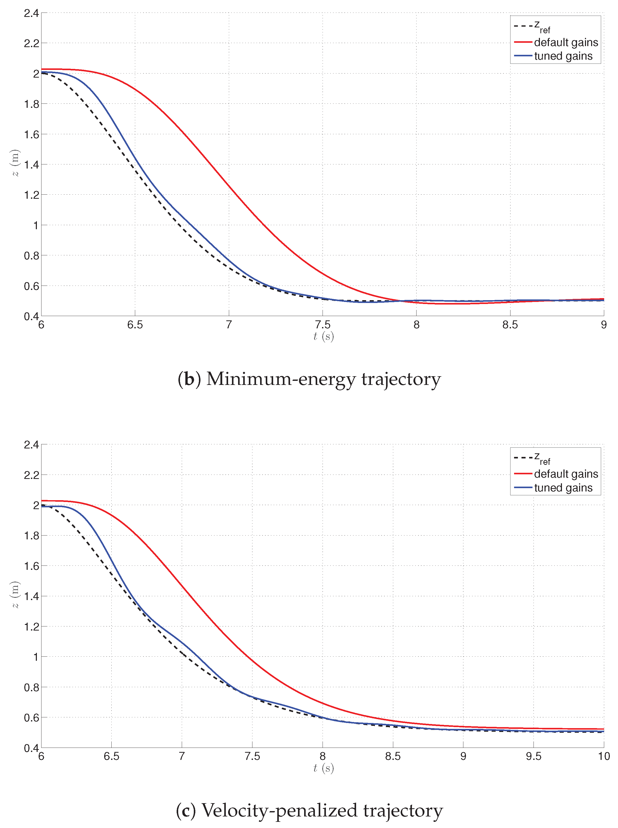
In this configuration of the controller, P and D gains of the altitude controller have been found by a systematic search within the admissible values’ ranges, repeating the experiment to ascend to $2\mathrm{m}$, hover, and descend the drone starting at $6\mathrm{s}$ from the altitude of $2\mathrm{m}$ to $0.5\mathrm{m}$, to observe possible overshoot effects. The gain values have been given in

Table 2. The gains used during the simulation.

Gains	Minimum-Time	Minimum-Energy	Velocity-Penalized
$K_p$	3.695	6.467	4.424
$K_d$	0.645	0.376	0.259

. The corresponding trajectories from the closed-loop system are presented in Figure 13.

10. Summary

In this paper, we demonstrated the applicability of the idea of optimization of the landing process of the UAV to the model-in-the-loop simulation of the Rolling Spider drone. The encouraging performance of the model of the system for various optimization criteria is shown through simulations. The obtained results imply that it is possible to design the control loop in such a way, so that various frequency responses of the closed-loop systems can be obtained, to shape the system’s response to a specific altitude reference signal. In order to do the latter, the altitude controller parameters need to be identified to ensure optimal-like behaviour.

In the future work, the authors plan to move from model-in-the-loop to hardware-in-the-loop experiments, using a motion capture system to precisely measure the altitude of the Rolling Spider drone, in comparison to the reference altitude. Such a knowledge enables one conduct further experiments with more complex approaches, including auto-tuning for real UAV experiment. Carrying out such experiments would make the method portable in the sense that it could also work for other types of UAVs, as just a reference profile and the tuning method need to be used.

On the other hand, it is to be stressed that for unstable structures, as presented in Reference [21], it is possible to build a composite feedback linearization control scheme where using an inverse dynamic model a reference trajectory generator is built, and the polynomial approximation of the trajectory is utilized, what calls for multivariable nonlinear programming problems to arise, to fit the polynomial into the waypoints. This might also be an interesting step, requiring good identification of the model, at first. As a wider and wider spectrum of the UAVs being constructed and successfully deployed, Reference [22], including a spectrum of control approaches, potentially enables researchers to identify new, optimal, control approaches to increase the performance of the flying structures at various stages of flight, including optimal landing procedure.