Abstract
The aim of this study is to optimize a four-cylinder, double-acting α-type Stirling engine with wobble-yoke mechanism using an optimization scheme incorporated with an efficient thermodynamic model. In this study, the non-ideal adiabatic thermodynamic model is improved by taking into account factors including pressure drops due to the sudden expansion or contraction of flow cross-sectional areas in the engine, multiple nodes in the regenerator adopted to accurately capture the temperature gradient in the regenerator, and the dependence of the transport properties (thermal conductivity and dynamic viscosity) of the working fluid on temperature and pressure. A parametric analysis is firstly performed to identify the designed parameters that need to be optimized. In this study, engine optimization is carried out by using the simplified conjugate-gradient method (SCGM). The effects of the weighting coefficients of the objective function are studied. For a particular case considered, the optimization successfully elevates the power output from 1062.56 to 1659.72 W, and thermal efficiency from 27.41% to 37.22%. Furthermore, the robustness of the optimization method is tested by giving different sets of initial guesses. It is found that the present approach can stably lead to the same optimal design and is independent of the initial guess.
1. Introduction
Two of the most critical issues in recent decades are the problems of global warming and energy crisis. These issues have been clearly addressed in a special report on global warming [1], which states that limiting global warming to a 1.5 °C target would require unprecedented changes in all aspects of society before unimaginable disasters happen. The report also suggested energy system transition as one significant change that needs to be made to combat climate change. In recent years, there has been a strong push to develop renewable energy options, such as solar energy and geothermal energy [2,3]. As an external combustion engine, the Stirling engine can be accommodated with various types of heat source. Egas and Clucas [4] presented a very detailed study on different engine configurations (alpha, beta and gamma) with rhombic-drive and Ross yoke mechanisms. It has been recognized that the Stirling engine is an effective power machine to harvest solar energy, geothermal energy and even waste heat in an environmentally friendly operation. For example, Sunpower Inc. developed a 9-kW free-piston Stirling engine to be used on a solar dish system, operated by Cummins Power Generation Inc., to harvest solar thermal energy [5].
In order to design a Stirling engine for delivering a high-power output, one would attempt to develop an engine with multiple cylinders. The four-cylinder double-acting α-type Stirling engine configuration shown in Figure 1 is one of the promising structures which has expansion and compression chambers located at different sides of each of the four pistons. The piston motion is affected by the pressures exerted on the upper and the lower faces of the piston, hence the name ‘double-acting’. One working zone of the double-acting Stirling engine connects the compression chamber of one cylinder through the flow ducts to the cooler, regenerator, heater and, finally, the expansion chamber of another cylinder. If this engine configuration is compared to four conventional α-type Stirling engines, the numbers of cylinders and pistons are reduced by half. This greatly increases the power density of the engine. With four cylinders, the phase angle of oscillation between two neighboring pistons is specified as 90°.
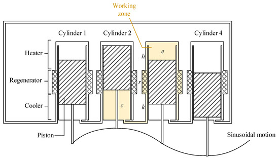
Figure 1.
Schematic of the four-cylinder double-acting α-type Stirling engine.
In 1977, Clucas and Raine [6] proposed a wobble-yoke mechanism that was used to drive the moving parts of the four-cylinder double-acting α-type Stirling engine. Later, García-Canseco et al. [7] proposed a model for control of the wobble-yoke Stirling engine. Chatterton and Pennacchi [8] have conducted a study on different multi-cylinder engine configurations and their thermodynamic performances. Urieli and Berchowitz [9] presented an ideal isothermal thermodynamic model and Yu et al. [10] presented a non-ideal adiabatic thermodynamic model to predict the performance of Stirling engines. Tan and Cheng [11] performed three-dimensional computational fluid dynamic analysis of the four-cylinder, double-acting Stirling engine using the wobble-yoke mechanism. A prototype engine (DASE1) was developed by Fung [12] in Power Engine and Clean Energy Lab., National Cheng Kung University, based on the same mechanism. The photograph of DASE1 is given in Figure 2.
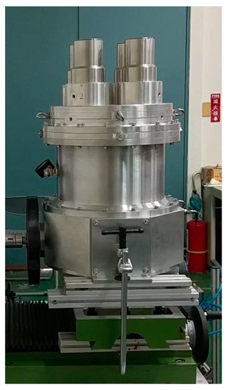
Figure 2.
Prototype engine, DASE1, developed by Power Engine and Clean Energy Lab., NCKU.
To the knowledge of the authors, prior to submitting the engine design for fabrication, computational optimization could help reduce the cost and time of manufacturing significantly, especially for an engine of higher power. Besides, due to the continuing improvements in computation technology, computational optimization has become an important tool to design the engines. For example, Ahmadi et al. [13] implemented the genetic algorithm for the optimization of a solar dish Stirling engine. This approach is a stochastic method which covers a global search of optimal geometrical parameters. However, it is less accurate and consumes more computation time. Hooshang et al. [14] describes the optimization of a gamma-type Stirling engine using neural networks as a pattern recognition tool to construct a mathematical model. This method requires a large amount of data for the neural network model to be accurate. On the other hand, Zare and Tavakolpour-Saleh [15] investigated the influence of dominant poles’ places on a free piston Stirling engine by means of the particle swarm optimization scheme.
The SCGM method is an optimization algorithm proposed by Cheng and Chang [16], which stemmed from the traditional conjugate-gradient method (CGM). The SCGM method simplifies the CGM method by giving a fixed step size value, and meanwhile the sensitivity analysis is done by adding perturbations to the designed parameters. In this manner, the relationship between the objective function and designed parameters can be determined without overwhelming the users with mathematical derivations. This method is well known and has been widely applied in the optimization of various engineering devices, such as fuel cell [17], thermoelectric cooler [18], and micro reformers [19].
The above literature survey has revealed the necessity of optimization of the Stirling engines. However, currently there exist only a few reports which are relevant to the optimization of the Stirling engine, not to mention the four-cylinder double-acting α-type Stirling engine. Under these circumstances, it is essential to develop an efficient numerical tool for designing this type of engine. In this study, the non-ideal adiabatic thermodynamic model [10] is modified and then incorporated with the SCGM method [16] so as to build a numerical optimization tool for this purpose. It is important to note that the application of the present approach includes but is not limited to the four-cylinder, double-acting α-type Stirling engine. The optimization method developed in this study is general and could be applied for the optimal design of any Stirling engine, provided that a direct problem solver like a thermodynamic or CFD model [12,20] has been developed. Detailed information about the present thermodynamic model and the optimization method is described in the subsequent sections.
2. Thermodynamic Model
In the thermodynamic model, only one working zone is considered, since these four cylinders will exhibit a periodic thermal and fluidic pattern from one another. In a typical working zone shown in Figure 1, the solution domain is divided into five sub-chambers, which are the expansion chamber, heater, regenerator, cooler and compression chamber. The piston displacement can be determined from the geometrical parameters of the wobble-yoke mechanism illustrated in Figure 3. Let the angles between the bottom surface of the wobble yoke arms and the horizontal plane be represented as and , for the expansion and the compression chambers, respectively, and the shaft rotation angles for the expansion and compression chambers be and . The values of and can be determined in terms of and as
where .

Figure 3.
Dimension variables of wobble-yoke mechanism.
Knowing , one can determine the piston displacement as
where . Then, the lengths of expansion and compression chambers can be calculated by taking point O as the origin.
The schematic of one working zone of the engine is plotted with the geometrical parameters in Figure 4. The volume of each chamber can then be calculated based on the lengths obtained above as
where and represent the dead space volumes, and is the regenerator’s porosity which is determined from the wire mesh geometrical parameters as
in which is the diameter of the mesh wire and is the wire pitch.
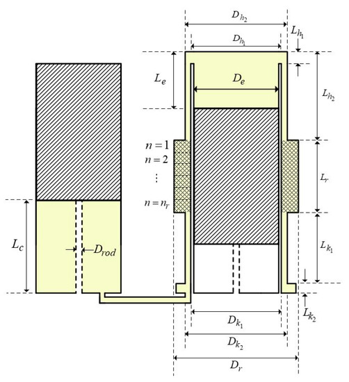
Figure 4.
Dimension variables of working zone.
Initial values for the pressure in all chambers are assumed to be equal and denoted as . The initial temperature of the expansion chamber and heater is assumed to be equal to the heater wall temperature, which is treated as the hot end temperature. The initial temperature of the compression chamber and cooler is assumed to be equal to the cooler wall temperature, which is the cold end temperature. Regarding the regenerator, multiple nodes are adopted to better predict the temperature gradient in the regenerator, as suggested in references [21,22]. The initial streamwise temperature profile in the regenerator is assumed to be a linear profile between the hot and the cold end temperatures. The use of multiple nodes can lead to a final streamwise temperature profile in the regenerator. Besides, the initial fluid temperatures in all the chambers are given as
where indicate the expansion chamber, heater, regenerator, cooler and compression chamber, respectively; is the number of nodes in the regenerator, and, in this study, typically is assigned to 40 after a node-number-independence check; and is the gas constant of the working fluid, helium.
The pressure variation in the working zone and the mass variations in all the chambers can be derived from the differentials of mass conservation equation, energy conservation equations and the ideal-gas equation of state. The results are given below
where and denote the temperatures at the interface at heater/expansion chamber and interface at compression chamber/cooler, respectively, which are given with upstream conditions based on the flow direction. The temperature variation in each chamber can be determined with the energy conservation equation as
where denotes the heat transfer between the walls and the working fluid in the control volume, the enthalpy change of working fluid, the output work by the working fluid, and the change in internal energy which equals mCvdT.
For the regenerator, the temperature of the solid matrix is determined from the energy balance as
The thermal resistances for heat transfer between the working fluid and the walls in the heater and the cooler are calculated in terms of the Nusselt numbers as
where and represent the Nusselt numbers on the surfaces of the heater and the cooler, respectively, which are calculated with the correlations provided in reference [23] for the flow in the circular-tube annulus, with a constant surface temperature on one surface and the other insulated.
Similarly, the thermal resistance between the working fluid and the solid matrix in the regenerator is
where the Nusselt number on the heat transfer area between the working fluid and the solid matrix is calculated by the correlations suggested by Rohsenow and Cho [24].
The temperature in the engine is varied from 300 to 1000 K. Meanwhile, the pressure in the engine is remarkably changed in a cycle, particularly in a highly pressurized engine. Therefore, the dependence of the transport properties (thermal conductivity kth and dynamic viscosity μ) of the working fluid on temperature and pressure is taken into account in the present model. The transport properties are expressed as functions of temperature and pressure based on empirical equations presented by Kuehl [25], as below. The coefficients in the following equation are tabulated in Table 1. The working volume density is calculated using the ideal gas equation of the state. The constant pressure and constant volume specific heat capacity are assumed as constant values.

Table 1.
Coefficients for the evaluation of helium’s dynamic viscosity and thermal conductivity. [25].
From Equation (21), fluid temperatures in the expansion and the compression chambers and in the regenerator at any instant of time can be determined with
Based on the obtained volumes and fluid temperatures in all the chambers, the average pressure can be calculated by using the ideal-gas equation of state as
Next, the average pressure is further corrected by considering pressure drops in each chamber. The friction coefficient in each chamber can be expressed as a function of Reynolds number. It is also noted that the influence of temperature has been taken into account in the dynamic viscosity and density terms in the calculation of Reynolds number. The empirical equations are taken from the existing report [26]. Moreover, since a real engine has connecting ducts of different sizes, additional pressure losses are expected due to a sudden expansion or contraction of the cross-sectional area of the ducts. For predictions of the pressure losses due to abrupt area change, the friction coefficients as functions of area ratios are obtained from references [27,28]. With the friction coefficients known, the pressure losses in all the chambers as well as the pressure losses due to abrupt area changes are calculated. Then, these pressure drops are introduced into the average pressure for the determination of the pressures in the expansion and the compression chambers as
The computation is started from the initial conditions described in the precedent section and is advanced to a stable regime eventually. After the stable regime is reached, then the power output and the thermal efficiency of the engine are calculated.
The test case of the thermodynamic model is specified with the prototype engine DASE1, whose parameters are listed in Table 1. Note that the charged mass of the working fluid, helium, in one working zone, is 63.4 mg to yield a cycle average pressure of approximately 4 bar, which is calculated using the ideal-gas equation of state by considering the charged pressure, initial volume and initial temperature in the engine chambers.
Next, a parametric analysis is performed to select the designed parameters. The effects of each parameter are evaluated using the thermodynamic model. In this section, the size of the engine and the charged mass of the working fluid are fixed. In addition, as a parameter is investigated, all other parameters are fixed at the given values displayed in Table 2. The results of the parametric analysis are plotted in Figure 5.
Table 2.
Specifications of the test case.
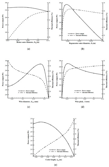
Figure 5.
Parametric analysis of the designed parameters. (a) Heater outer diameter; (b) Regenerator outer diameter; (c) Wire diameter; (d) Wire pitch; (e) Cooler length.
Figure 5a shows the effects of the heater outer diameter on the engine indicated power output and thermal efficiency. The magnitude of thermal efficiency increases with the outer diameter and finally reaches a maximum of 33.97% at = 0.071 m. On the other hand, the curve for the indicated power output exhibits a peak value at = 0.0683 m. It is clear that the peak values of the two curves appear at different heater outer diameters. A peak exists with a curve because when the heater outer diameter is small, an increase in the heater outer diameter leads to an increase in the heat transfer surface area at the top of the cylinder and in the heater annular flow duct volume as well. Over the peak, the performance of the engine descends due to the excessive dead volume with larger heater outer diameter.
The effects of the regenerator outer diameter on the engine performance are depicted in Figure 5b. Again, one observes two different regenerator outer diameters: one corresponds to highest power output and another one to the highest thermal efficiency. This is because a certain amount of wire mesh is required to carry out heat transfer between the solid matrix and the working fluid. However, as continues to grow, the dead volume and the pressure losses due to abrupt area changes also increase.
The effects of the wire diameter and wire pitch of the wire mesh used for making the regenerator are shown in Figure 5c,d, respectively. A change in wire diameter or the wire pitch of the regenerator affects the regenerator’s porosity. The porosity then affects the dead volume of the working chamber and the heat transfer between the fluid and solid matrix of the regenerator. In Figure 5c, it is seen that there is an optimal wire diameter for the maximum indicated power output, whereas the curve for thermal efficiency does not exhibit a peak value. In Figure 5d, an optimal wire pitch for maximum indicated power output is found at λ = 0.15 mm, and again the curve for thermal efficiency does not exhibit a peak value.
Finally, the effects of the cooler length on the engine performance are conveyed in Figure 5e. Since the height of the engine is fixed, a change in cooler length is accompanied by a change in the heater length. In this figure, an optimal value of the cooler length exists for the highest indicated power output, while the thermal efficiency increases with the cooler length monotonically.
3. Thermodynamic Model vs CFD Model
On the other hand, CFD models can lead to more detailed and complete information of the flow and thermal fields, which is not easily obtained with the thermodynamic model. However, one major concern about the CFD analysis is its time consumption in the computation. To estimate the time consumption in the CFD analysis of the present Stirling engine, a CFD computation has also been performed for the test case. Detailed information regarding the numerical schemes used was described in detail by Cheng and coauthors [12,20].
Figure 6 shows the comparison in indicated power output as a function of engine speed between the thermodynamic model and the CFD analysis. Close agreement between the two sets of data is clearly seen in this figure. Note that the readings of the power output in Figure 6 are delivered by only a working zone. With a four-cylinder double-acting engine, the total power output is four times the reading given in this figure. This implies that the engine can produce a total power output of approximately 1.2 kW at 2000 rpm.
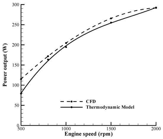
Figure 6.
Comparison between thermodynamic model and CFD analysis in indicated power output.
A comparison between the temperature from the thermodynamic model and the volume-average temperature from the CFD analysis may be helpful. Figure 7 shows that there exists a small discrepancy between the two sets of temperature data. Nonetheless, the trend of the curves is nearly the same and the maximum difference in temperature is acceptable.
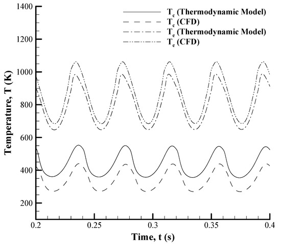
Figure 7.
Comparison in expansion and compression chambers’ temperature variations.
A comparison in computation time between the two models is shown in Table 3. The computations are executed on a personal computer with Intel Xeon CPU E5-2620 v3 processor. It is seen that, for a typical test case, the CFD model needs more than 52 h to finish 20 cycles in simulation, whereas the thermodynamic model requires only 1 min. In the optimization process, the number of iterations could exceed 200, and hence it is not practical to choose the CFD model as the direct problem solver. According to the comparison described above, the validity of the developed thermodynamic model is basically confirmed, and therefore the thermodynamic model is chosen as the direct problem solver for the optimization, instead of the CFD model.
Table 3.
Consumed computation time by thermodynamic and CFD models.
4. Optimization Method
This study intended to develop an efficient approach for optimizing the engine by integrating the developed thermodynamic model and the SCGM method [16]. As the baseline design of this engine is readily available, local optimization is carried out to improve the engine performance while keeping the original engine configuration. Thus, the SCGM method is chosen for its deterministic approach and fast convergence.
In addition, the approach is modified for a multi-goal optimization, in which the objective function is defined such that the indicated power output and the thermal efficiency can both be increased at the same time. For this purpose, the objective function is defined as the reciprocal of the sum of indicated power output and thermal efficiency in the following
where in the right-hand side, the denominator of the fraction includes two terms. The magnitude of the indicated power output is represented by the first term, and the magnitude of thermal efficiency second term. The two positive weighting coefficients, c1 and c2, are prescribed by the users based on the design purpose. Note that c1 + c2 = 1.0. The effects of different combinations of c1 and c2 are investigated later.
In this study, a set of k designed parameters are optimized simultaneously. Let {Xj|j =1 , 2, 3, …, k} denote the designed parameters to optimize. The minimization of the objective function will be achieved in the iterative process. By means of the SCGM method [16], the set of the designed parameters are given initial values by the specifications of the prototype engine, and then the optimal values will be yielded in iterations. The thermodynamic model is adopted as a direct problem solver to predict the indicated power output and the thermal efficiency of the engine, corresponding to the updated designed parameters. The direct problem solutions are sent back to the SCGM code in order to calculate the objective function by Equation (33) and then to update the designed parameters. The designed parameters are updated by
where the step size (), and the search direction () are calculated at every iteration with the following equations
For the first iteration, the step size is given a constant value and the conjugate gradient coefficient is assigned to be zero. With the variable step size calculated from Equation (35), the optimization iteration can speed up as the gradient of search direction is large and slow down as the search approaches the optimal design.
The conjugate gradient coefficient is calculated by
where the gradient functions (∂Jj/∂Xj, j = 1, 2, 3, …, k) are determined by a direct numerical sensitivity analysis: First, a perturbation (ΔXj) is added to each of the designed variables, and then the change in the objective function (ΔJj) caused by ΔXj is determined. The gradient function with each designed variable is approximated by numerical differentiation: ∂Jj/∂Xj = ΔJj/ΔXj.
The optimization process is terminated as the objective function reaches its minimum value. Therefore, the process is completed as the relative error of objective functions between two consecutive iterations is decreased to be less than 10−9. The coupling of the optimization method with the thermodynamic model is shown in Figure 8.
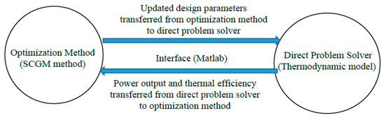
Figure 8.
Connection between optimization method and thermodynamic model.
5. Results and Discussion
In the parametric analysis shown in Figure 5, only one parameter is changed, while the others are fixed in each plot. In fact, multi-parameter optimization is more practical from a designer’s viewpoint. The five parameters considered in Figure 5 exhibit peaks on the performance curves of the engine, and hence, as a test of the present approach, they are all selected to be the designed parameters to optimize simultaneously. Their original values are listed in Table 4.
Table 4.
Designed parameters and their original values.
The optimization is carried out under some geometrical constraints. For example, the outer diameters of heater and cooler cannot exceed a critical value, 0.08 m. The sum of the lengths of the heater and cooler is fixed at 0.144 m. The wire diameter of the wire mesh used in the regenerator should always be less than the wire pitch. The regenerator’s porosity, which can be expressed in terms of wire diameter and wire pitch, should always be between 0 and 1. These constraints are tabulated in Table 5.
Table 5.
Geometrical constraints.
It is important to mention that in the present approach, all the parameters of the engine are categorized into designed, fixed and dependent parameters. The relationship between the dependent and the designed parameters must be clearly defined and expressed as the constraint equations shown in Table 5. If, for example, parameter a is actually another form of parameter b, one simply needs to figure out the constraint (relationship) between a and b. Therefore, other than the highly independent parameters, this model works for inter-dependent parameters by incorporating constraints among the parameters.
Firstly, the magnitudes of the weighting coefficients are set to be c1 = 0.3 and c2 = 0.7. The optimal search for the combination of the design parameters is in the direction of decreasing objective function. Figure 9 shows the variation in the objective function in the optimization process. It is seen that the value of the objective function indeed is continuously decreased. For this case, the iteration number to reach the optimal designs is less than 250, and the lowest value of the objective function is approximately 0.0067.
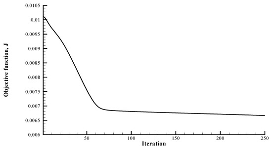
Figure 9.
Minimization of objective function in the optimization process.
The comparison of P-V diagrams between the original and optimal designs is illustrated in Figure 10. It is seen that the areas of the cycles on P-V diagrams in the both the expansion and the compression chambers are indeed enlarged remarkably. The expansion in the areas of the cycles reveals the improvement in the power output of the engine by optimization. The results of the optimal set of the designed parameters and the engine performance before and after the optimization are tabulated in Table 6. Using the present optimization approach, the indicated power output can be increased from 1062.56 to 1659.72 W, and the thermal efficiency from 27.41% to 37.22%.
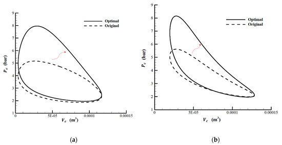
Figure 10.
P-V diagrams of the original and optimal designs. (a)Expansion chamber; (b) Compression chamber.
Table 6.
Optimal designed parameters and performance improvement.
It is seen in Table 6 that the heater outer diameter tends to increase for a larger heat transfer surface area, but it is limited by the increase in dead volume. The regenerator outer diameter approaches the outer diameter of both heater and cooler so that the pressure drop due to the sudden expansion and contraction of the flow is minimized. This can be seen also in the literature [29], where the pressure drop due to the sudden expansion and contraction of flow is minimized when the heater, regenerator and cooler diameters are almost the same. The wire mesh parameters are optimized so that this leads to the optimum porosity. The cooler length increases, while the heater length reduces, because the thermal resistance at the cold side is higher than that of the hot side.
Influence of changing the weighting coefficients c1 and c2 on the optimal design’s performance is evaluated and the results are displayed in Table 7. The main purpose of the optimization program is to maximize the indicated power output without reducing the thermal efficiency. Three different combinations of c1 and c2 are considered here. As stated earlier, the coefficients may be selected depending on the design purposes. By elevating the value of c1, the emphasis on the power output improvement is stronger, so that the power output is expected to become higher. As shown in this table, as the value of c1 is increased from 0.15 to 0.5, the indicated power output is elevated from 1615.56 to 1663.12 W, while the thermal efficiency is slightly reduced from 37.54% to 36.37%. The results provided in Table 7 agree with this expectation.
Table 7.
Effects of weighting coefficient on the optimal design’s performance.
With this approach, the initial guess can be varied arbitrarily to a certain extent. It is important to know whether the optimization method leads to a unique optimal point as the initial guess is changed. Thus, three additional initial guess sets are adopted in addition to the previous case (initial guess 1). Figure 11 shows the trajectories of the optimization process from the four sets of initial guesses in the space of (, , ). The values of the parameters associated with the four initial guesses and the optimal point are tabulated in Table 8. It is clearly seen that, even though the initial guesses are separated in the space, the approach always finds the same optimal point. It means that the approach is robust and independent of the initial guess. Note that the approach is not just limited to the present group of designed parameters. When necessary, more designed parameters may be added in the group. Using more designed parameters actually means that the optimization can be done in a bigger search space so that a better solution can be expected. If the group of designed parameters are changed, the optimization requires a separate convergence study. The approach presented in this report is of great potential for the practical design of the Stirling engine.
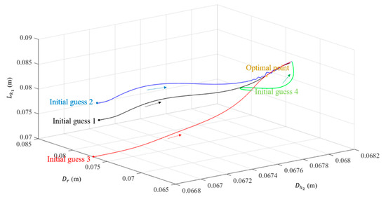
Figure 11.
Convergence trajectory of different sets of initial guesses.
Table 8.
Numerical values of initial guesses and the optimal point.
It is important to note that the present optimization method is capable of modifying an existing original design so as to reach a higher performance. However, the side effect of manufacturing, mechanical properties may be possible. One possible manufacturing problem would be that the optimized parameters of the parts may not be commercially available. If that is the case, to reduce the cost, one can pick commercialized parts close enough to the optimized geometrical parameters.
6. Conclusions
In this study, an optimization approach based on thermodynamic modelling incorporated with the SCGM method has been successfully developed to optimize the geometrical parameters of a four-cylinder double-acting α-type Stirling engine using the wobble-yoke mechanism.
The thermodynamic model is built by modifying an existing non-ideal adiabatic thermodynamic model. The validity of the developed thermodynamic model has been confirmed with a three-dimensional computational fluid dynamics analysis. The approach can continuously adjust the combination of the designed parameters in order to minimize the objective function.
After optimization, the indicated power output can be increased from 1062.56 to 1659.72 W, and the thermal efficiency from 27.41% to 37.22%.
Finally, the robustness of the optimization method is tested using different initial guesses. The results show that the approach is robust and independent of the initial guess for a typical case.
In conclusion, the approach presented in this report is of great potential for the practical design of the Stirling engine.
Author Contributions
Conceptualization, C.-H.C.; methodology, C.-H.C. and Y.-H.T.; software, Y.-H.T.; validation, C.-H.C. and Y.-H.T.; formal analysis, C.-H.C. and Y.-H.T.; investigation, C.-H.C. and Y.-H.T.; resources, C.-H.C..; data curation, Y.-H.T.; writing—original draft preparation, Y.-H.T.; writing—review and editing, C.-H.C.; visualization, Y.-H.T.; supervision, C.-H.C.; project administration, C.-H.C.; funding acquisition, C.-H.C. All authors have read and agreed to the published version of the manuscript.
Funding
This research was funded by the Ministry of Science and Technology, Taiwan, under Grant MOST 108-3116-F-006 -014 -CC2.
Conflicts of Interest
The authors declare no conflict of interest.
References
- Global Warming of 1.5 °C: An IPCC Special Report on the Impacts of Global Warming of 1.5 °C above Pre-Industrial Levels and Related Global Greenhouse Gas Emission Pathways, in the Context of Strengthening the Global Response to the Threat of Climate Change, Sustainable Development, and Efforts to Eradicate Poverty; Masson-Delmotte, V., Zhai, P., Pörtner, H.-O., Roberts, D., Skea, J., Shukla, P.R., Pirani, A., Moufouma-Okia, W., Péan, C., Pidcock, R., et al., Eds.; IPCC: Geneva, Switzerland, 2018. [Google Scholar]
- Kongtragool, B.; Wongwises, S. A Review of Solar-Powered Stirling Engines and Low Temperature Differential Stirling Engines. Renew. Sustain. Energy Rev. 2003, 7, 131–154. [Google Scholar] [CrossRef]
- Kolin, I.; Koscak-Kolin, S.; Golub, M. Geothermal Electricity Production by Means of the Low Temperature Difference Stirling Engine. In Proceedings of the World Geothermal Congress, Tohoku, Japan, 28 May–10 June 2000. [Google Scholar]
- Egas, J.; Clucas, D. Stirling engine configuration selection. Energies 2018, 11, 584. [Google Scholar] [CrossRef]
- Stine, W.B.; Diver, R.B. A Compendium of Solar Dish/Stirling Technology; No. SAND-93-7026; Sandia National Labs.: Albuquerque, NM, USA, 1994. [Google Scholar]
- Clucas, D.; Raine, J. The WhisperGen: A Strategy for Commercial Production. In Proceedings of the 8th International Stirling Engine Conference, Ancona, Italy, 27–30 May 1997; pp. 159–168. [Google Scholar]
- García-Canseco, E.; Alvarez-Aguirre, A.; Scherpen, J.M. Modelling for Control of a Wobble-Yoke Stirling Engine. In Proceedings of the 2009 International Symposium on Nonlinear Theory and its Applications NOLTA’09 2009, Sapporo, Japan, 18–21 October 2009; pp. 544–547. [Google Scholar]
- Chatterton, S.; Pennacchi, P. Design of a Novel Multicylinder Stirling Engine. J. Mech. Des. 2015, 137, 042303. [Google Scholar] [CrossRef]
- Urieli, I.; Berchowitz, D.M. Stirling Cycle Engine Analysis; Adam Hilger Ltd.: Bristol, UK, 1984. [Google Scholar]
- Yu, Y.X.; Yuan, Z.C.; Ma, J.Y.; Zhu, Q. Numerical Simulation of A Double-Acting Stirling Engine in Adiabatic Conditions. Adv. Mater. Res. 2012, 482, 589–594. [Google Scholar] [CrossRef]
- Tan, Y.H.; Cheng, C.H. Simulation of Performance of a Four-Cylinder Double-Acting α-Type Stirling Engine. In Proceedings of the 18th International Stirling Engine Conference (ISEC), Tainan, Taiwan, 19–21 September 2018. [Google Scholar]
- Fung, T.Y. Theoretical Analysis and Design of Double Acting Four-Cylinder Stirling Engine. Master’s Thesis, National Cheng Kung University, Tainan, Taiwan, 2017. [Google Scholar]
- Ahmadi, M.H.; Sayyaadi, H.; Mohammadi, A.H.; Barranco-Jimenez, M.A. Thermo-Economic Multi-Objective Oprimization of Solar Dish-Stirling Engine by Implementing Evolutionary Algorithm. Energy Convers. Manag. 2013, 73, 370–380. [Google Scholar] [CrossRef]
- Hooshang, M.; Moghadam, R.A.; Nia, S.A.; Masouleh, M.T. Optimization of Stirling Engine Design Parameters Using Neural Network. Renew. Energy 2015, 74, 855–866. [Google Scholar] [CrossRef]
- Zare, S.; Tavakolpour-Saleh, A.R. Applying particle swarm optimization to study the effect of dominant poles places on performance of a free piston Stirling engine. Arab. J. Sci. Eng. 2019, 44, 5657–5669. [Google Scholar] [CrossRef]
- Cheng, C.H.; Chang, M.H. A Simplified Conjugate-Gradient Method for Shape Identification Based on Thermal Data. Numer. Heat Transf. Part B Fundam. 2003, 43, 489–507. [Google Scholar] [CrossRef]
- Jang, J.Y.; Cheng, C.H.; Huang, Y.X. Optimal Design of Baffles Locations with Interdigitated Flow Channels of a Centimeter-Scale Proton Exchange Membrane Fuel Cell. Int. J. Heat Mass Transf. 2010, 53, 732–743. [Google Scholar] [CrossRef]
- Huang, Y.X.; Wang, X.D.; Cheng, C.H.; Lin, D.T.W. Geometry Optimization of Thermoelectric Coolers Using Simplified Conjugate Gradient Method. Energy 2013, 59, 689–697. [Google Scholar] [CrossRef]
- Cheng, C.H.; Huang, Y.X.; King, S.C.; Lee, C.I.; Leu, C.H. CFD-based Optimal Design of a Micro-Reformer by Integrating Computational Fluid Dynamics Code using a Simplified Conjugate-Gradient Method. Energy 2014, 70, 355–365. [Google Scholar] [CrossRef]
- Cheng, C.H.; Chen, Y.F. Numerical Simulation of Thermal and Flow Fields inside a 1-kW Beta-Type Stirling Engine. Appl. Therm. Eng. 2017, 121, 554–561. [Google Scholar] [CrossRef]
- Yuan, S.W.K.; Spradley, I.E.; Yang, P.M.; Nast, T.C. Computer Simulation Model for Lucas Stirling Refrigerators. Cryogenics 1992, 32, 143–148. [Google Scholar] [CrossRef]
- Ataer, Ö.E.; Karabulut, H. Thermodynamic Analysis of the V-type Stirling-Cycle Refrigerator. Int. J. Refrig. 2005, 28, 183–189. [Google Scholar] [CrossRef]
- Ackermann, R.A. Cryogenics Regenerative Heat Exchangers; Springer Science & Business Media: New York, NY, USA, 1997. [Google Scholar]
- Rohsenow, W.M.; Cho, Y.I. Handbook of Heat Transfer; McGraw-Hill: New York, NY, USA, 1998. [Google Scholar]
- Kuehl, H.D. Numerically Efficient Modelling of Non-Ideal Gases and their Transport Properties in Stirling Cycle Simulation. In Proceedings of the 17th International Stirling Engine Conference and Exhibition (ISEC), Newcastle Upon Tyne, UK, 24–26 August 2016; pp. 572–579. [Google Scholar]
- Kays, W.M.; London, A.L. Compact Heat Exchangers; McGraw-Hill: New York, NY, USA, 1984. [Google Scholar]
- Streeter, V.L. Handbook of Fluid Dynamics; McGraw-Hill: New York, NY, USA, 1961. [Google Scholar]
- Fried, E.; Idelchik, I.E. Flow Resistance: A Design Guide for Engineers; Taylor & Francis: New York, NY, USA, 1989. [Google Scholar]
- Hamaguchi, K.; Yamashita, I.; Hirata, K. Effects of Sudden Expansion and Contraction of Flow on Pressure Drops on the Stirling Engine Regenerators. In Proceedings of the 33rd Intersociety Energy Conversion Engineering Conference (IECEC-98-100), Colorado Springs, CO, USA, 2–6 August 1998. [Google Scholar]
© 2020 by the authors. Licensee MDPI, Basel, Switzerland. This article is an open access article distributed under the terms and conditions of the Creative Commons Attribution (CC BY) license (http://creativecommons.org/licenses/by/4.0/).