Abstract
Seasonal storage of thermal energy, by pumping heated water through a borehole array in the summer, and reversing the water flow to extract heat in the winter, can ameliorate some of the intermittency of renewable energy sources. Simulation can be a valuable tool in enhancing the efficiency of such storage systems. This paper develops a simple, efficient mathematical model of spatial temperature dynamics that focuses on the radial water flow in a cylindrical borehole array. The model calculates the time course of the temperature difference between outgoing and incoming water accurately, and allows new optimization strategies to be explored easily. A strategy based on discharging water heated by the array before it reaches the array center can increase the storage capacity by 25% for a system with a 20% smaller radius than the well-studied Drake Landing system. If the density of boreholes is also doubled, the improvement is 29%.
1. Introduction
A major obstacle to extensive deployment of renewable energy sources is their intermittency, both daily and seasonal. The daily variations may eventually be addressed using batteries. However, for seasonal storage to be economically feasible, the cost needs to be on the order of $1 per kWh [1], about two orders of magnitude below current battery prices. Borehole thermal energy storage (BTES) [2,3,4] is much less expensive. During the summer, hot water from sources such as rooftop solar collectors is pumped into a short-term storage tank. Hot water from the tank is then pumped into the center of an array of U-shaped pipes in boreholes (Figure 1a), typically with a uniform spacing. As the water travels to the edge, it deposits heat in the soil. When the water leaves the borehole array, it is transported back to the storage tank to be reheated, and then reenters the array. The flow of water is reversed in the winter, so that heated water exits at the center, where the water is hottest. It is then used to heat the short-term storage tank, from which water is taken to heat homes. The round-trip storage efficiency (ratio of heat taken out to heat put in) is typically around 50% or less due to losses from thermal diffusion [2,4].
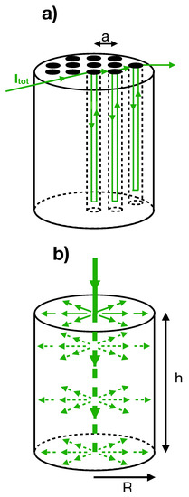
Figure 1.
(a) Water flow (green) during charging of BTES system. One of several lines of boreholes leading from the center to the boundary is drawn. Boreholes toward the front of the array are omitted for clarity of viewing. (b) Schematic of model with radial water flow.
Most current BTES systems are still too expensive for widespread application [5]. Therefore, several simulation studies aimed at enhancing efficiency have been performed. Many of these [4,6,7,8,9,10] have have embedded symmetrized borehole temperature fields in a global temperature field (via the “Duct-Storage” or DST approximation) using packages such as TRNSYS [11]. Several have treated the Drake Landing system [4,12] in Ototoks, Alberta, in which 54 homes are heated by an array of 144 boreholes, 35 m deep. McDowell and Thornton [6] treated the entire system, including solar collectors, the short-term storage tanks, the load from the homes, and the BTES. They optimized system parameters in the design phase to achieve 90% of the home heating energy to come directly from solar collectors or from the storage. The number of solar collectors, the size of the short-term storage tanks that were used, and the number and depth of the boreholes for the ground storage were varied to find the combination that maximized the economic performance. The model was subsequently tuned to initial data for the system. Within the BTES system, varied ground properties included the thermal conductivity and the heat capacity. This resulted in a reduction of the thermal conductivity by 35% relative to the original estimate and an increase of the heat capacitance by about 30%. With these parameters, an excellent fit was obtained to the output water temperature both during charging and discharging over the four-month fitting period. Later, these calculations were extended to treat the first five [8] and ten [4] years of operation. The calculated BTES efficiencies (ratio of heat taken out to heat put into the array) were typically within 20% of the measured values. Rad et al. [10] used TRNSYS with a custom BTES component based on the “GHEADS” method [13] to design a system along the same line as the Drake Landing one, but more cost-effective. By using a different design of short-term storage tank, along with fewer and deeper boreholes, they achieved a configuration expected to outperform the Drake Landing one at a cost 19% lower.
Other possible installation types and operational strategies have also been investigated. Zhang et al. [9] studied the application of a BTES system with 25 boreholes to heating a greenhouse of area 231 m using TRNSYS-DST. It was found that the BTES plus solar collector system could reduce the auxiliary heat requirement by about 80% relative to a system with no storage. Chapuis and Bernier [7] created a TRNSYS model of a system operating at a temperature too low for direct space heating of homes, in which each borehole had two separate circuits so that charging and discharging could occur simultaneously. The low temperature reduces losses from thermal diffusion. The system was supplemented by heat pumps to heat homes. A cost–benefit analysis relative to the Drake Landing installation was not made, but with a greatly reduced number of collectors coupled to an increased BTES volume it was still possible to obtain a solar fraction of about 80%.
The full three-dimensional (3D) geometry of the BTES has also been treated using finite-element methods. Simulations have explored the dependence of the BTES efficiency on properties such as borehole spacing and diameter, soil thermal diffusion coefficient, and water permeability. Zhang et al. [14] used the TOUGH2 finite-element method [15] to model the Drake Landing system. The method apparently was unable to treat changes in flow direction over the scale of hours, thus instead each year was divided into 21 periods during which charging or discharging was uniform (or vanishing); the same scheme was used for all years. It appears that a priori assumed parameter values were used rather than being adjusted to fit the data. This approach described the qualitative features of the temperature profiles reasonably well, but the calculated output temperature could be off by more than 8 in some cases. Catolico et al. [16] also applied TOUGH2 to the Drake Landing system, but added several features including a larger dataset for temperature comparison, modified soil parameters to fit the data better, and the use of different charging schemes for different years. Systematic variation of parameters in the model allowed them to conclude that: (i) the heat extraction efficiency decreases with increasing soil thermal conductivity, groundwater flow, and soil permeability; and (ii) unsaturated soils show higher overall heat extraction efficiency. Calculations for a smaller system [17], performed using the COMSOL package (COMSOL Inc: Stockholm, Sweden) [18], found a low storage efficiency due to thermal diffusion. Welsch et al. [19] used the FEFLOW finite-element program [20] to investigate possible improvements from using borehole arrays significantly deeper than those developed thus far. They found that efficiencies as high as 80%, much higher than current values, could be achieved. The main source of the increased efficiency was the rise of the soil temperature with increasing depth.
Current approaches to optimizing BTES design via simulation are limited in several ways. First, they use trial-and-error approaches to find new designs, which means that whole new avenues of improvement may be ignored. Improvements on these approaches could be made if there were a known explicit, simple relationship between the BTES efficiency and key properties of the BTES, such as geometry, soil thermal properties, and borehole spacing/diameter. Such a relationship will be of the greatest value if it is derived from a model that is known to be accurate, but it is hard to glean such relationships from the relatively complex simulation methods that are currently being used. Simpler, more physically transparent approaches, make it easier to derive such relationships. In addition, few direct comparisons of theoretical models with experimental time courses, including short-time fluctuations, have been published. Standard quantitative measures of quality of fit, such as rms difference between theory and experiment, have not been provided. This makes it hard to evaluate the reliability of the modeling methods. Finally, there has been little physical analysis of features seen in the data, such as characteristic peaks seen at the onset of charging.
These observations motivated the derivation of simpler, physically transparent, and computationally efficient models. They are not expected to be as accurate as some existing approaches, but they can have significant advantages in modeling and designing BTES systems. Computational efficiency simplifies: (i) exploration of a broad range of design options; and (ii) parameterization of the model to fit experimental data. It also allows the use of a time step small enough to treat rapid variations in flow and temperature, which is important for model validation. Furthermore, conceptually simple models have a larger base of potential users. Finally, the physical transparency of such models allows the relationships between key design parameters and system behavior to be seen more clearly. Some of these advantages are obtained by the “Earth Energy Designer” package [21], which utilizes stored results of previous heat-transfer calculations of “g-functions” to speed up the analysis process. This has been used in systematic studies of the effect of design parameters on efficiency [22]. However, the range of application of this method is limited by the range of stored results. Furthermore, it does not treat short time scales.
Here, a simplified, physically transparent model based on coarse-graining the borehole-field geometry is developed. It is shown that the model accurately describes data from the Drake Landing Solar Community [4,12] over time scales ranging from years to less than an hour, with an rms error of less than 1 C. Characteristic features seen in the temperature time course are interpreted in terms of a transiently enhanced heat-transfer coefficient and the time required for the temperature distribution to reach a quasi-steady state for a given soil–temperature distribution. The model is then used to develop a modified charging strategy, based on discharging water when it reaches a certain temperature as opposed the standard approach of always discharging from the center of the array. The modified approach increases the efficiency relative to standard charging strategies by: (i) 25% in systems that are 20% smaller in radius than the Drake Landing one; (ii) 15% in systems with twice the borehole density of the Drake Landing system; and (iii) 29% in systems that have both reduced system size and increased borehole density relative to the Drake Landing system. Because the size of BTES installations is limited by available land, improving the efficiency of smaller systems is particularly advantageous.
2. Methodology
The system treated has a total water current flowing through an array of U-shaped pipes (Figure 1a), placed in boreholes with uniform spacing a in a cylindrical region. From the central boreholes, paths linking the boreholes emanate outward. The paths do not follow straight lines along the radial direction, which would result in a lower density of boreholes toward the edge of the array. Rather, they also have lateral connections, particularly near the edge, which allow a constant density of boreholes to be achieved. A typical path layout is shown in Ref. [23].
The model coarse-grains this system, treating it as a cylinder of radius R and height h oriented along the z-axis (Figure 1b).
The complex up, down, and sideways flow pattern of the individual pipes is replaced by a continuous radial flow of water, described by a volume fraction w and a speed that decreases toward the cylinder edge. Heat is exchanged between the water and the soil, and diffuses in the soil with coefficient D. The model treats: (i) the coarse-grained temperature of the soil, averaged over the region closest to a particular borehole; and (ii) the average temperature of all the water in a borehole, also treated as a continuous variable.
The key simplifying assumptions of the model are:
Radial water flow dominates the temperature dynamics. To assess the validity of this approximation, it is useful to consider the “plug” of water initially contained in the upward-and downward going pipes of the central borehole in Figure 1a. The average z-coordinate of this plug is halfway up the cylinder. As the plug moves out through the borehole array, does not change appreciably because water moving from the upward pipe to a neighboring borehole occupies the z-range previously occupied by the water in the downward-moving pipe. The pipes connecting the boreholes are much shorter than the boreholes, so their contribution can be neglected.
Therefore, the average motion of the water is primarily in the r-direction; the motion in the z-direction serves mainly to equalize water and soil temperature in this direction. The velocity is taken to have the form
so that is constant as a function of r. Appendix A.1 shows that average time required for the water to reach a distance r is obtained correctly by Equation (1), if . This provides support for Equation (1), since and the soil–temperature distribution jointly determine how much heat has been transferred at the distance r.
Vertical variations of soil and water temperature inside the cylinder can be ignored. This assumption is supported by the calculations of Ref. [16], which show much larger soil–temperature variations in the radial direction than in the vertical direction. The average water temperature of the two pipes in a borehole also is likely to have limited vertical variation: the upward and downward water currents have temperature gradients in opposite directions, which will cancel.
Heat flow between water and soil is proportional to :
where is a rate parameter. This assumption becomes accurate for sufficiently slow variations in flow or temperature [24]. Appendix A.2 presents numerical calculations of the time evolution of the temperature gradient at a pipe boundary after a sudden temperature jump, using a circularized approximation of the borehole geometry (Figure A1 and Figure A2). Calculations of the heat flow resulting from this gradient show that Equation (2) holds to within 20% for a time-independent already when . For the parameters of the model, day. Thus, Equation (2) should describe seasonal temperature variations very well, and diurnal variations moderately well.
However, the flow often changes on a scale of hours, too fast for Equation (2) to be accurate. When flow is suddenly turned on, the initial heat-transfer rate is very high because there are large temperature gradients at the soil–water interface. This effect is included by transiently increasing after flow changes:
The function is chosen so that correctly describes a sudden flow jump (see Appendix A.2), using Equations (A4) and (A5).
The resulting model equations inside the cylinder are
where the Laplacian is two-dimensional (2D) and + and − in Equation (5) describe discharging and charging, respectively; describes heat flow from soil to water. The soil volume fraction is chosen to be unity, since as is shown below. Since the heat flowing into the soil equals the heat flowing out of the water, , where and are the volumetric heat capacities.
The embedding of the cylinder into the surrounding three-dimensional soil medium is described in Appendix A.3. Space is divided into a “cylinder” region and an “external” region, and separate solutions for these regions are matched continuously at a boundary . Heat transfer at the bottom of the cylinder is treated by the addition of a term proportional to (Equation (A11)) in the cylinder region, where is the asymptotic soil temperature away from the cylinder. The exterior solution (Equation (A13)) includes the spreading of heat in 3D instead of 2D, as well as heat transfer at the soil–air interface.
The model equations are simplified by assuming that reaches steady state rapidly for a given distribution and fixed values of and , so that in Equation (5):
where approaches exponentially with a spatial rate . Because the soil temperature changes very slowly, the steady-state approximation should hold on time scales larger than the time required for the water to traverse the array, which from Equation (A1) is about 30 min in the case of the Drake Landing installation.
3. Results and Discussion
3.1. Description of Drake Landing data
Numerical solutions of Equations (3), (4), (6), (A11) and (A13) are used to simulate the Drake Landing dataset [12], which covers the period 1 July 2007 to 30 June 2017. The borehole spacing is m, while m and m. Each of 24 lines of boreholes has a length 432 m of pipes with radius cm, thus . C is taken from McDowell and Thornton [6], who obtained by fitting to the temperature data from Drake Landing. This indirect measurement was used because to our knowledge there are no direct representative measurements of the heat capacity at Drake landing. There is a substantial uncertainty in this value; McDowell and Thornton [6] had originally estimated , while the authors of [14,16] used . The known value C was used. The time step is 10 min, the same as the interval between data points in the Drake landing results. A simulation for one set of parameters takes less than a minute to run on a MacBook Air laptop. Further details of the calculations are given in Appendix A.4.
The flow of water through the short-term storage tank is not explicitly treated. Instead, the focus is on energy-storage properties of the borehole array itself. These are determined by the flow rate and the difference between the incoming and outgoing water temperatures. The latter are taken from temperature sensors near the pipes. The time-dependent initial conditions for Equation (6), (charging) or (discharging), are taken from the sensors nearest and . During charging and discharging the model equations are used to calculate and , respectively, and the model is fitted by comparing these predictions to the data. The flow velocity at the cylinder edge is obtained as , where is obtained from the dataset. An asymptotic soil temperature of 8 C is assumed at large distances, as in Ref. [16].
The two adjustable parameters D and are fit to data for Years 7–10 of the dataset, taken at 10-min intervals. The number of data points during which the system is charging or discharging is about 140,000 for each sensor. The initial distribution of is taken from simulations for Years 1–6. Years 7–10 are chosen to minimize effects of the initial conditions before charging starts. The optimal values are and ; as mentioned above, . Previously measured D values for wet clays of about [25] are smaller than the fitted value. However, the exact nature of the soil at Drake Landing is uncertain, and the effective D obtained here could be higher because of convective effects being larger than believed. Fully 3D simulations based on information from the vicinity of the Drake Landing area [14,16] took .
Figure 2 compares the model predictions, averaged over weekly periods, with the data for Years 7–10. Figure 3 shows 10-min data for selected 20-day periods. The model fits the data closely, with a 0.8 C rms deviation. Even rapid variations in are obtained accurately by the full model including the time dependence of and (Equation (3)). For example, in Figure 3a, at time days, charging is turned on abruptly. The ensuing gradual rise in is captured accurately by the full model, but not by a model (turquoise points) with constant and , which gives a more constant temperature after charging begins. The gradual rise in the full model occurs because and are enhanced right after charging begins; this causes a rapid exponential decay of the temperature change along the path of the water, which means that the temperature jump is strongly attenuated at the output. In physical terms, immediately after charging is turned on, the initial heat pulse is absorbed near the input, because heat is transferred very rapidly until the quasi-steady state temperature distribution for the current soil–temperature distribution is built up. The model correctly also predicts that the diurnal oscillations in during charging (Figure 3a) are much smaller than those in , but it still overestimates their magnitude. The quality of fit here appears to be comparable to that of Ref. [6], and better than that of Refs. [14,16].
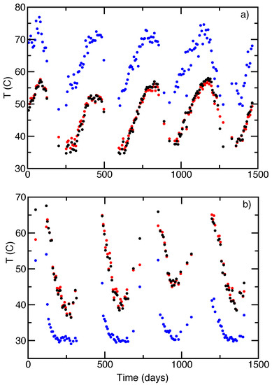
Figure 2.
Week-averaged model predictions vs. measured temperatures. Day 1 is 1 July 2013 and days begin at midnight. Red and black dots: model predictions and experimental data for (charging) and (discharging). Blue dots: initial condition (charging) or (discharging). (a) Charging periods. (b) Discharging periods.
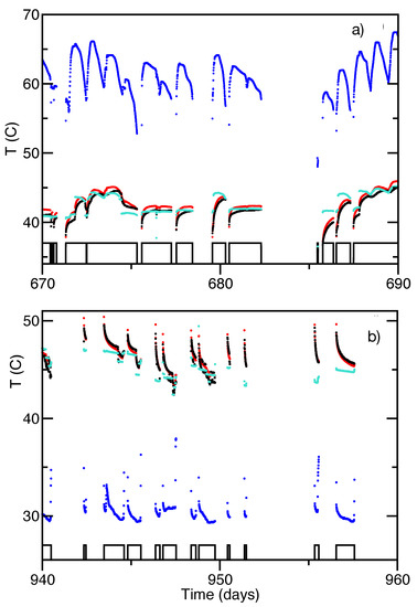
Figure 3.
Model predictions on ten-minute time mesh vs. measured temperatures. Red, black, and blue are as in Figure 2. Black boxes show charging and discharging periods. (a) Charging periods. Black boxes denote beginning and end of charging periods. Turquoise curve is temperature time course obtained for a time-independent . (b) Same as (a), but during discharging periods.
The model radial water-temperature profiles at representative times of charging and discharging (Figure 4a) also fit the data well.
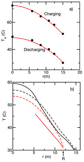
Figure 4.
(a) Theoretical (red) vs. experimental (black) temperature profiles. Charging is at days (05:50 on 6 June 2016); discharging is at days (13:00 on 14 January 2016). (b) (black) and (red) for constant-temperature discharge strategy (solid lines) and baseline discharge strategy (dashed lines), in simplified model. System size is reduced by 20% (R = 12 m) and w is twice the baseline value. Solid curve ends at m because water is discharged there ().
3.2. Exploration of Potential Improvements to Model
This validation of the model motivates using it to predict the effects of some possible modifications that might enhance the energy-storage capacity of the system. For simplicity, it is assumed that half the year is spent charging at a constant input temperature 66 C, and the other half is spent discharging at a lower input temperature 31 C. These choices are motivated by the Drake Landing data. The power demand during discharging is taken to have the form
where is a prefactor, is the peak discharge time, and is the width of the charging peak. This form fits the Drake Landing data better than a constant . The peak time is taken to be halfway through the discharging period, while a fit to the data gives days. Constant values of and are used since the variations in the charging rate are slow and the input temperatures are constant.
The stored-energy function embodies the key physical effect that “all heat is not equal”: transferred heat has greater value if the transfer occurs at a higher temperature difference. For example, a furnace that heats air by only a few degrees is ineffective because of the large airflow required to transfer the heat. The effect of the temperature difference is incorporated by requiring that the outlet and intake temperatures during discharge satisfy , where . Then, the power taken out of the system is
where is the unit step function, while the available stored energy is
Here, and define the discharging period in Year 10, which is far enough into the simulation that steady state is reached. C is chosen larger than the typical temperature jump of ∼10 C in a forced-air heat pump, in order to account for incomplete heat transfer. The value of in Equation (7) is chosen as the highest value that allows the -criterion to be satisfied throughout the entire discharging period. It is obtained by incrementing upwards until the criterion fails to be satisfied.
In existing BTES installations, the density of boreholes is constant and water enters the system during discharge at the boundary and leaves at the center. Fluctuating power demand is met by varying either the fraction of time spent discharging or the flow rate. The model mimics this baseline approach by: (i) taking to be constant; (ii) taking and ; and (iii) taking . The efficiency for this case is slightly below 50%, comparable to that at Drake Landing.
Two alternatives to this approach were explored:
- (i)
- A nonuniform borehole spacing, treated via an r-dependent w. Conservation of water then requires that . Several possible shapes of were tried, including both increasing and decreasing Gaussians, and step-function shapes with either a higher or lower central value of w. A decreasing Gaussian, for example, would describe a borehole spacing that is larger near the edge of the array. None of these shapes increased by more than 2%, thus a constant borehole spacing seems to be nearly optimal.
- (ii)
- Discharging heated water before it reaches the array center. Water entering at is discharged not at , but already at the point defined by at a particular time. Thus, at all times. The varying demand is met by taking . During charging, water enters at and leaves at . could be varied by placing outlet valves at various radii in the array, and adding pipes to connect different circuits at a given radius. This procedure “sculpts” the soil–temperature profile, removing heat preferentially from the edge of the array. This is denoted the “constant-temperature” discharge strategy.
Figure 4b shows the sculpting effect of strategy (ii) at , for a reduced system size and doubled value of w. The constant-temperature approach lowers the soil temperature at the edge. This lowering mitigates the temperature gradient at the edge and thus reduces the diffusive heat loss. Because of the soil–water interaction, the lowered in turn brings down during charging. This increases the charging power, which is proportional to .
The constant-temperature strategy always increases , sometimes by a large fraction (see Table 1). The increase depends on the size of the system and the borehole density (described by w). It is 6% for the size and borehole density of Drake Landing. However, it can be over 20% for a smaller system size and/or an increased borehole density. Thus, using this strategy might enhance the practicality of smaller systems. Even larger enhancements are obtained if is constant rather than peaked as a function of time.

Table 1.
Stored-energy capacity (in GJ) for different discharge strategies. CT denotes constant-temperature. m is the radius of the Drake Landing system.
About 50–70% of the increase in results from increased charging energy, and the rest from reduction in diffusive loss. The increase in the charging energy and decrease in diffusive loss are both between 1% and 4%. The percent increase in exceeds the sum of these changes because diffusive heat loss cancels a large part of charging energy. For example, the efficiency of 40–50% at Drake Landing [4] implies a cancellation of 50–60%. The cancellation increases at smaller system sizes, enhancing the effect of the discharge strategy.
4. Conclusions and Future Work
The main findings of the paper are the following:
- (i)
- A conceptually simple and physically transparent model of a BTES array, treating only outward flow of water, heat transfer between soil and water, and thermal diffusion of water, gives an accurate description of the water-temperature dynamics. This physically transparent model, based on Equations (3), (4), (6), (A4), (A11) and (A13), runs quickly and is simple enough that it can be straightforwardly coded within generally available packages such as MATLAB, Fortran, and C. This greatly expands the range of possible users, and simplifies the simulation of new types of system configurations, such as the recently proposed “zone” strategy [22,26]. Application of the model to the Drake Landing BTES installation [4,12] gives a fit to the measured temperature data, for both the long-term trends and more rapid fluctuations, with an rms error of less than 1 C. This quality of fit equals or exceeds those of previous models. The model provides a useful complement to more complete approaches such as TRNSYS [11] and finite-element calculations.
- (ii)
- The model predicts that a modified discharge strategy for water heated by the soil can increase the energy-storage capacity significantly. This strategy involves removing water heated by the array at a point where it has been heated by a fixed degree difference rather than using the conventional approach of removing the water at the array center. This new strategy reduces diffusive losses and increases the energy put into the system during charging. The storage capacity is increased by 25% in systems that are 20% smaller in radius than the Drake Landing one, 15% in systems with twice the borehole density of the Drake Landing system, and 29% in systems with both reduced system size and increased borehole density. This may enhance the practicality of smaller BTES systems, which are particularly sensitive to thermal diffusion. This is an important improvement, since BTES size is limited by available land, and these findings may shift the balance toward smaller systems with a higher density of boreholes. It also enhances the likelihood of a BTES system being practical for a single multiunit building. Since the market for underground thermal energy storage could be several hundred billion dollars in the US alone [1], even small efficiency improvements could be very significant.
These improvements are comparable in magnitude to some other approaches that have been proposed. Rad et al. [10] found that a change in the geometry to increase the aspect ratio of the borehole array led a a cost reduction of about 20%, while maintaining the storage capacity of the Drake Landing system. The design of Chapuis and Bernier [7] used a lower-temperature version of the Drake Landing system in combination with heat pumps. The borehole volume was increased by a factor of four relative to the Drake Landing system. This allowed the solar panel area to be reduced by 75%, with a solar fraction of about 80% as opposed to the over 90% solar fraction at Drake Landing. Because the costs of acquiring, installing, and running the heat pumps were not treated, it is difficult to compare this approach head-on with the present one. Welsch et al. [19] found that using boreholes about an order of magnitude deeper than the ones at Drake Landing could lead to a round-trip efficiency of 80% or more, significantly higher than the roughly 50% efficiency at Drake landing. Because there must be large costs associated with such deep drilling, it is again difficult to compare these improvements head-on with the ones proposed here.
The key limitations of the BTES model in its present form are the following:
- (i)
- The coarse-graining and symmetrization of the borehole field give a description of the temperature field that is in principle less accurate than can be obtained by finite-element simulations. However, finite-element simulations at this point do not appear to be fast enough to treat the rapid flow and temperature fluctuations that occur in typical BTES installations. Therefore, the method presented here seems to be a good choice for describing these rapid variations.
- (ii)
- The coarse-graining of the model means that the identification of points in the model with particular boreholes, for temperature comparisons, is imprecise. However, the temperature variation from borehole to borehole is quite slow, so this is probably not a major concern.
- (iii)
- The model is limited to installations with near-cylindrical symmetry. This is likely not a major limitation, since systems with other symmetries, such as rectangular or triangular, would likely lose more heat by diffusion and thus be less efficient. In principle, a spherical system might have smaller diffusive losses because it minimizes surface area, but this appears to be impossible given that only straight boreholes can be drilled.
- (iv)
- The model is only applicable to installations with a large number of boreholes. In smaller systems, the coarse-graining approximation will not be accurate.
- (v)
- Since the model does not treat water flow in the soil induced by temperature gradients, it is only applicable to cases where this flow has small thermal effects. This is believed the case for the Drake Landing system [16], but further study is needed.
- (vi)
- The model does not treat the effects of changes in individual borehole properties, such as the thermal properties of the U-tubes. It only has a two global parameters describing heat transfer, which are fitted to the experimental data.
- (vii)
- The validity of the assumptions made in embedding the two-dimensional diffusion inside the cylinder into the three-dimensional surrounding soil is not known. However, the insensitivity of the results to the details of the embedding, in particular to the embedding radius, suggests that this is not a large problem.
- (viii)
- The “constant-temperature” discharging approach has been tested only on a scenario based on two constant input temperatures, one for charging and one for discharging. To qualitatively evaluate the effectiveness of the approach in more complicated scenarios, it is worth noting that the importance of the soil-sculpting effect depends strongly on the combination of the exponential decay rate characterizing the convergence of water temperature to the soil temperature, and the cylinder radius. According to Equation (6), this combination is captured by the dimensionless parameter . If discharging is turned on and off frequently, will be enhanced immediately after the times when discharging is turned on, suggesting the the effect will be more important during those times. Thus, the overall effect could to enhance the boost in storage capacity from the constant-temperature discharging scenario, although the effect should be small because it only occurs during the transients before the steady-state is reached.
Future work should pursue the following directions:
- (i)
- Systematic testing of the “constant-temperature” discharging approach using more complex input temperatures profiles.
- (ii)
- Inclusion of soil permeability and water flow effects. It may be possible to treat soil permeability via an enhancement of the thermal diffusion coefficient, so that one number treats both thermal diffusion and permeability effects. This should be a useful approximation since a temperature gradient generates a pressure gradient that drives a flow of water, which in turn generates a flow of heat—a process parallel to the direct diffusion of heat. Effects of directed water flow across the entire system could be approximately treated by adding a non-radial component to . For example, for water flow in the x-direction, one could write . Then, starting with an initially circularly symmetric state (), water flow in the x-direction would cause to build up. Once has built up, further water flow would result in feeding back on .
- (iii)
- Relating the global heat-transfer parameters and D to the detailed properties of the boreholes and the pipes. This could be done by fitting the model to more complete results obtained via finite-element methods, for shorter run times and/or smaller systems.
- (iv)
- Further analysis and simplification to obtain an explicit formula for the energy-storage capacity. A reasonable scale for the energy-storage capacity is , where is the average input water temperature during charging, is the average input water temperature during discharging, and V is the volume of the system. This is the energy that would be stored if all of the the soil temperature reached the incoming water temperature, and if the discharging water brought the final soil temperature down to the input water temperature during discharging. It is clearly an overestimate. An accurate expression for the energy-storage capacity for a cylindrical BTES might have the form , where g is a dimensionless function and and are the times spent charging and discharging, respectively. Extensive simulation runs using a model of the type described here, along with further efforts toward simplification, will help pin down the form of this function.
Funding
This research received no external funding.
Acknowledgments
Natural Resources Canada/CanmetENERGY supplied extensive data for the Drake Landing installation. Valuable input from Lucio Mesquita and Yu-Feng Lin is appreciated.
Conflicts of Interest
The author declares no conflict of interest.
Nomenclature
| Symbol | Definition | Drake Landing or Baseline Value |
| R | Array radius | 15 m |
| Baseline R | 15 m | |
| Water discharge radius | varies | |
| h | Array height (borehole depth) | 35 m |
| w | Water volume fraction | 0.000206 |
| Water volume specific heat | C | |
| Soil volume specific heat | C | |
| Total water current | Varies | |
| Water current density | Varies | |
| D | Soil thermal diffusion coefficient | |
| Coarse-grained water temperature | Varies | |
| Coarse-grained soil temperature | Varies | |
| Asymptotic soil temperature | ||
| Incoming water temperature in simplified model | , | |
| Outgoing water temperature in simplified model | Varies | |
| Minimum temperature increase in constant-volume discharge strategy | ||
| Time required for water to reach radius r | Varies | |
| Time required for water quasi-steady-state to be reached | 6 h | |
| Time width of discharge peak in simplified model | days | |
| Time of peak discharge in simplified model | years | |
| Start time of discharge in simplified model | years | |
| Stop time of discharge in simplified model | years | |
| Water heat-transfer coefficient | Varies | |
| Soil heat-transfer coefficient | Varies | |
| Steady-state soil heat-transfer coefficient | ||
| Steady-state water heat-transfer coefficient | ||
| Enhancement factor for and | Varies | |
| Power demand at time t in simplified model | Varies | |
| Peak power value in simplified model | Varies |
Appendix A
Appendix A.1. Validity of Equation (1)
The validity of Equation (1) is established by comparing two calculations of , the average time for water beginning at the center of the array to reach a distance r from the center. This quantity is crucial because it determines how much heat has been transferred to or from the flowing water at a distance r.
- Discrete approach using actual 3D borehole geometry with boreholes in a square array of spacing a and height h, laid out in circuits starting at the center. If , then the number of boreholes inside r is . Since , the total length of pipe inside r is well approximated as (the factor of 2 accounts for the upward-flowing and downward-flowing pipes in each borehole). The average length of each circuit going out from the center to the radius r is then , where is the number of circuits. If the velocity of water in the pipes is , then the average time for the water to reach r is thus
- Continuous model approach based on radial flow (Equation 1). The flow velocity is obtained from the total current carried by the pipes. The fractional water density is , where the factor of 2 again comes from the “upward” and “downward” pipes in each borehole and is the pipe radius. Then, from , one finds . The average time required to reach r is thus
Appendix A.2. Validity of Equation (2) and Implementation of Equation (3)
First the soil–temperature dynamics following a sudden change in flow are calculated. It is assumed that a sudden change in flow leads to an equally sudden change in temperature. When there is no flow, the water is at the temperature of the surrounding soil. When flow turns on, the temperature where the water enters the array jumps quickly, because the time required to get from the hot-water reservoir to the BTES array is short, since the water comes from a short-term storage tank close to the borehole array.
Thus, as a first step, the soil–temperature dynamics are calculated following a step-function change in in a borehole: . The change is initially assumed to be uniform along the borehole, but below a correction to this approximation is described. The calculations use an approach similar to that of Ref. [24], which builds on the general theory described in Ref. [27]. This approach generalizes to 2D the familiar one-dimensional analysis of the temperature evolution in a slab with temperatures fixed at both ends [28], where is expanded in trigonometric functions with appropriate boundary conditions.
The behavior in the square set of of points closest to a single borehole (see Figure A1) is calculated approximately.

Figure A1.
Schematic of circularized model of the environment of a borehole (top view).
Figure A1.
Schematic of circularized model of the environment of a borehole (top view).

To obtain a mathematically tractable formulation, the square region of side a is replaced by a circular region of radius having the same area as the square, thus placing each borehole inside a cylinder of radius and height h. The up- and down-going pipes of radius are replaced by a single pipe of radius having the same area as the two pipes. Only circularly averaged quantities are treated, since is circularly averaged over the cylinder, and non-circular components will only interact weakly with the water in the pipes because the pipe radius is small.
The radial coordinate is denoted by and the thermal diffusion equation is solved, taking from the assumption of continuity of the temperature at the boundary. At , it is assumed that . This is justified because of the small average heat current at the boundary. From a typical temperature difference of between and 15 m, the estimate is obtained. The total heat power entering the cylinder due to diffusion is . However, this also equals the total boundary heat current , where the derivative is the average value along the boundary. Therefore, . By comparison, the typical value of is , which is much larger than the gradient. This justifies the zero-slope boundary condition.
is expanded in a basis of eigenfunctions of , satisfying and at :
where and are cylindrical Bessel functions, the are chosen so that for each n the radial derivative at vanishes, and the are constant coefficients. The form in Equation (A3) satisfies the diffusion equation since and ; it also automatically vanishes at .
The are evaluated numerically, finding for example and . The are found from the initial condition at , using orthogonality properties of the Bessel functions. is obtained by numerical integration. The resulting time dependence of the dimensionless heat-transfer coefficient is shown in Figure A2. The coefficient is large at small times but is within 20% of its asymptotic value already when or .
The use of a single pipe of radius to treat the two pipes in a borehole is not quantitatively justified. However, the results are relatively insensitive to the choice of , having a slow logarithmic dependence. Since the results are insensitive to size, it is likely that they are insensitive to shape as well.

Figure A2.
Dimensionless heat-transfer coefficient vs. time, obtained by numerical evaluation of Equation (A3).
Figure A2.
Dimensionless heat-transfer coefficient vs. time, obtained by numerical evaluation of Equation (A3).

The results in Figure A2 are used to determine the factor in Equation (3), which describes the increase in occurring after rapid changes in flow. It is calculated as
where is a delay function that integrates to unity and is a small correction included to avoid singularities when the integral vanishes. Shortly after a sudden jump in from zero to a positive value, the denominator is less than , thus ; for a constant , . Thus, is enhanced immediately after a current jump, and returns to the value after the flow has been stable for a long time.
The function is chosen such that correctly describes a step function jump in from 0 to 1, with the enhancement factor obtained from the data in Figure A2. Ignoring the term, a change of variables in the denominator of Equation (A4) gives . Therefore,
To implement this result, the approximate analytic form
is used, where . This fits the data in Figure A2 very closely.
This analysis treats an infinitely long pipe with a spatially uniform temperature jump. However, the change in the soil temperature distribution must propagate from one end of the pipe to the other, which slows the convergence of and to their asymptotic long-time values. To account for this effect, the amount of heat transfer required for to come down to a certain value along an entire pipe is calculated, and then the time it takes for the incoming water to accomplish this transfer is calculated. This value is chosen to be , and (=11,100 s) is defined as being the time when reaches in the uniform case.
The power transmitted from the water to the soil per unit length of pipe is
Numerical integration of the data in Figure A2 shows that
so the total heat required for to drop to is
where is the length of pipe in the system (again using the single-pipe approximation).
The total heat power entering the system from the incoming water is approximately . Thus, the time required to transfer the heat into the system is
It is assumed that the total time required to get down to is . The extra time is accounted for in the calculations by stretching the time axis in the function in Equation (A4) by a factor of = 1 + 51,460/11,100 = 5.64.
Appendix A.3. Corrections to Cylindrical-Diffusion Model
Three physical effects are added to the two-dimensional diffusion model in Equation (4): heat loss through the bottom of the cylinder, three-dimensional spreading, and heat transfer from soil to air outside the cylinder area.
Heat loss through the bottom of the cylinder (the heat loss through the top is much lower because it is insulated) is treated by assuming that the heat current density flowing out from each point on the bottom equals the steady-state heat current density from a sphere of radius R and temperature , where is the asymptotic soil temperature away from the borehole array. This leads to an additional term in :
The factor of h in the denominator accounts for spreading of the heat loss out over the height of the cylinder, by the up-and-down water flow. This term is included only when .
Outside the cylinder, diffusion becomes three-dimensional, and heat is lost at the soil–air interface. These effects are treated by matching the two-dimensional calculation to a three-dimensional calculation at a crossover radius . The soil–air heat transfer is modeled via a constant-temperature condition at the boundary, as in Ref. [16]. For conceptual simplicity, the asymptotic soil temperature is used, which is close to the average surface temperature of [16]. The constant-temperature condition implies that the heat current flows perpendicular to the boundary everywhere. Therefore, the temperature distribution has a dipole form at large distances, proportional to the Legendre polynomial , where is the angle measured relative to the cylinder axis. (This can be understood by mathematical analogy with electrostatics, in which the electric field surrounding a charge dipole is perpendicular to the plane bisecting the dipole.) In general, the Laplacian for angular dependence defined by a given Legendre polynomial is
Therefore, since here, it is assumed that outside ,
is taken to correspond to a sphere of volume equal to that of the cylinder. Since this choice is not rigorously justified, other values of been chosen, which give a comparable fit. Using (17% lower) gives an rms error of , while using a value equal to the distance from the cylinder center to the top of the cylinder edge (28% higher) gives an rms error of . The baseline error is .
Appendix A.4. Additional Details of Calculations
- (1)
- Thermal diffusion. The thermal properties of the borehole grout are assumed to be similar to those of the soil. The soil at Drake Landing is probably wet clay [16], with a thermal conductivity of roughly [25]. Cementitious grouts containing twice as much sand as cement have [29]. The grout at Drake Landing has a slightly lower proportion of sand, which increases the thermal conductivity. Thus, should be less than 2.4 , supporting the assumption. Convective heat transfer in the soil is ignored. The analysis of Ref. [16] indicated that thermal diffusion, as opposed to convection, is the dominant mode of heat dispersion.
- (2)
- Numerical procedures and fitting. Equation (6) was integrated by using a local linear approximation to in each interval . This gives an analytic solution on the interval involving an exponential. The end value of on each interval was used as the starting point for the next interval. A step size of m was found to give good convergence. The diffusion equation was solved using a nearest-neighbor approximation to the 2D Laplacian, using a time step of 10 min. The optimal values of D and were found by calculating the root-mean-square error over a 2D mesh of possible values. The total squared error was obtained by adding up the squares of the residuals between the theoretical predictions and the experimental data (97,358 charging data points and 49,870 discharging data points). Data for were taken from the “23-1” sensor; was from the “23-7” sensor in the dataset [12]. Data in Figure 4a were taken from sensors “23-1” to “23-7”.
References
- Jacobson, M.Z.; Delucchi, M.A.; Cameron, M.A.; Frew, B.A. Low-cost solution to the grid reliability problem with 100% penetration of intermittent wind, water, and solar for all purposes. Proc. Natl. Acad. Sci. USA 2015, 112, 15060–15065. [Google Scholar] [CrossRef] [PubMed]
- Rad, F.M.; Fung, A.S. Solar community heating and cooling system with borehole thermal energy storage–Review of systems. Renew. Sustain. Energy Rev. 2016, 60, 1550–1561. [Google Scholar] [CrossRef]
- Lanahan, M.; Tabares-Velasco, P. Seasonal thermal-energy storage: A critical review on BTES systems, modeling, and system design for higher system efficiency. Energies 2017, 10, 743. [Google Scholar] [CrossRef]
- Mesquita, L.; McClenahan, D.; Thornton, J.; Carriere, J.; Wong, B. Drake Landing Solar Community: 10 Years of Operation. In Proceedings of the ISES Solar World Congress 2017, Abu Dhabi, UAE, 29 October–2 November 2017. [Google Scholar]
- Reed, A.; Novelli, A.; Doran, K.; Ge, S.; Lu, N.; McCartney, J. Solar district heating with underground thermal energy storage: Pathways to commercial viability in North America. Renew. Energy 2018, 126, 1–13. [Google Scholar] [CrossRef]
- McDowell, T.P.; Thornton, J.W. Simulation and model calibration of a large-scale solar seasonal storage system. Proc. SimBuild 2008, 3, 174–181. [Google Scholar]
- Chapuis, S.; Bernier, M. Seasonal storage of solar energy in borehole heat exchangers. In Proceedings of the Eleventh International IBPSA Conference, Glasgow, UK, 27–30 July 2009. [Google Scholar]
- Sibbitt, B.; McClenahan, D.; Djebbar, R.; Thornton, J.; Wong, B.; Carriere, J.; Kokko, J. The performance of a high solar fraction seasonal storage district heating system—Five years of operation. Energy Procedia 2012, 30, 856–865. [Google Scholar] [CrossRef]
- Zhang, L.; Xu, P.; Mao, J.; Tang, X.; Li, Z.; Shi, J. A low cost seasonal solar soil heat storage system for greenhouse heating: Design and pilot study. Appl. Energy 2015, 156, 213–222. [Google Scholar] [CrossRef]
- Rad, F.M.; Fung, A.S.; Rosen, M.A. An integrated model for designing a solar community heating system with borehole thermal storage. Energy Sustain. Dev. 2017, 36, 6–15. [Google Scholar] [CrossRef]
- Klein, S.; Beckman, W.; Mitchell, J.; Duffie, J.; Duffie, N.; Freeman, T.; Mitchell, J.; Braun, J.; Evans, B.; Kummer, J.; et al. TRNSYS 17: A Transient System Simulation Program; Solar Energy Laboratory, University of Wisconsin: Madison, WI, USA, 2010. [Google Scholar]
- Natural Resources Canada (Ottawa, ON, Canada); CanmetENERGY (1615 Boulevard Lionel-Boulet, Varennes, QC J3X 1P7, Canada). Personal communication, 2018.
- Rad, F.M.; Fung, A.S.; Leong, W.H. Effects of weather parameters on vertical ground heat exchanger design. ASHRAE Trans. 2014, 120, 184–195. [Google Scholar]
- Zhang, R.; Lu, N.; Wu, Y.s. Efficiency of a community-scale borehole thermal energy storage technique for solar thermal energy. In Proceedings of the GeoCongress 2012: State of the Art and Practice in Geotechnical Engineering, Oakland, CA, USA, 25–29 March 2012; pp. 4386–4395. [Google Scholar]
- Pruess, K.; Oldenburg, C.M.; Moridis, G. TOUGH2 User’s Guide Version 2; Technical Report; Lawrence Berkeley National Lab. (LBNL): Berkeley, CA, USA, 1999.
- Catolico, N.; Ge, S.; McCartney, J.S. Numerical modeling of a soil-borehole thermal energy storage system. Vadose Zone J. 2016, 15. [Google Scholar] [CrossRef]
- Başer, T.; Lu, N.; McCartney, J.S. Operational response of a soil-borehole thermal energy storage system. J. Geotech. Geoenviron. Eng. 2015, 142, 04015097. [Google Scholar] [CrossRef]
- COMSOL Inc. COMSOL Multiphysics Version 5.4; COMSOL Inc.: Stockholm, Sweden, 2018. [Google Scholar]
- Welsch, B.; Ruehaak, W.; Schulte, D.O.; Baer, K.; Sass, I. Characteristics of medium deep borehole thermal energy storage. Int. J. Energy Res. 2016, 40, 1855–1868. [Google Scholar] [CrossRef]
- Diersch, H.J.G. FEFLOW: Finite Element Modeling of Flow, Mass and Heat Transport in Porous and Fractured Media; Springer: Berlin, Germany, 2013. [Google Scholar]
- Hellström, G.; Sanner, B. Earth Energy Designer; Blocon AB: Lund, Sweden, 2000. [Google Scholar]
- Skarphagen, H.; Banks, D.; Frengstad, B.S.; Gether, H. Design Considerations for Borehole Thermal Energy Storage (BTES): A Review with Emphasis on Convective Heat Transfer. Geofluids 2019, 2019, 4961781. [Google Scholar] [CrossRef]
- Borehole Thermal Energy Storage (BTES). Available online: http://https://www.dlsc.ca/borehole.htm (accessed on 22 November 2019).
- Hellstrom, G. Ground Heat Storage Thermal Analysis of Duct Storage Systems. Ph.D. Thesis, Department of Mathematics Physics, Lund University, Lund, Sweden, 1991. [Google Scholar]
- Chesworth, W. Encyclopedia of Soil Science; Springer: Berlin, Germany, 2007; p. 167. [Google Scholar]
- Borehole Thermal Energy Storage. Available online: https://www.phcppros.com/articles/6989-borehole-thermal-energy-storage (accessed on 18 February 2019).
- Carslaw, H.S.; Jaeger, J.C. Conduction of Heat in Solids, 2nd ed.; Clarendon Press: Oxford, UK, 1959. [Google Scholar]
- Lienhard, J.H. A Heat Transfer Textbook; Courier Corporation: North Chelmsford, MA, USA, 2013. [Google Scholar]
- Allan, M.; Philippacopoulos, A. Performance characteristics and modelling of cementitious grouts for geothermal heat pumps. In Proceedings of the World Geothermal Congress, Kyushu, Tohoku, Japan, 28 May–10 June 2000; Volume 28. [Google Scholar]


© 2020 by the author. Licensee MDPI, Basel, Switzerland. This article is an open access article distributed under the terms and conditions of the Creative Commons Attribution (CC BY) license (http://creativecommons.org/licenses/by/4.0/).