Market Trading Model of Urban Energy Internet Based on Tripartite Game Theory

Abstract

As an important driving force to promote the energy revolution, the emergence of the energy internet has provided new ideas for the marketization and flexibility of multi-energy transactions. How to realize multi-energy joint trading is a key issue in the development of the energy market. An urban energy internet market trading model among energy suppliers, energy service providers and the large users in the urban area, based on tripartite game theory, is established in this paper. Considering the cost–income function of each market entity and the basic market trading mechanism, a new game-tree search method is proposed to solve the Nash equilibria for the game model. The Nash equilibria of the tripartite game can be obtained, and the market transaction status corresponding to the Nash equilibria is analyzed from the perspective of the market transactions. The multi-energy joint transaction and market equilibria can be easily implemented for the bids and offers of the multiple energy entities in the urban energy internet market.

1. Introduction

Energy consumption is an important basis for socio-economic development. As traditional fossil energy sources are gradually depleted, how to achieve efficient energy use has become a major problem all over the world. Combining the use of electricity, heat and natural gas may be a promising way to deal with the energy consumption efficiency issue. Therefore, the concept of energy internet was proposed [1,2]. Energy internet is a complex multi-energy flow system that has a power system as the core, the internet and other cutting-edge information technologies as the foundation and distributed renewable energy as the main energy source, and is closely coupled with thermal systems, natural gas networks, transportation networks and other systems [3]. Based on the basic characteristics of multi-energy-coupled energy internet, the main goal of the energy internet market is to achieve multi-energy comprehensive transactions. In order to better realize complementary use of multiple energy sources and improve energy efficiency, it is particularly important to establish a multi-time scale, multi-energy, energy internet market trading model [4]. Compared with the pure electrical energy trading in the traditional electricity market, other energy sources such as thermal energy will also be included in the multi-energy market, and the trading behavior of market entities will affect the entire trading mechanism [5].

Up to the present, the pure electricity market [6,7,8,9] has been relatively mature, and the research on the multi-energy market trading models has also been gradually carried out. A real-time and day-ahead level equilibrium model of the electricity and natural gas markets was established, and a special diagonalization algorithm was proposed in [10]. A day-ahead market settlement framework considering the uncertainty of renewable energy was presented in [11]. Few studies have been conducted on the trading of multiple energy types, considering the competition strategies among multiple market entities. In particular, the trading models of multi-market entities such as energy suppliers, energy service providers and large users within an urban level energy internet have not yet been well resolved [12].

As a commonly used method in the field of economics, game theory [13,14,15] has become an important means to solve the strategies for competing market entities related to the Nash equilibria. For example, an electricity market game model between the microgrid and distribution network was proposed in [16], in which the entities within a microgrid formed a cooperative alliance to conduct the electricity transactions with the distribution network. [17] grouped many independent microgrids together and conducted a price-bidding game with the remaining power-surplus microgrids. A distributed demand-side energy management system was established in [18], and the interaction between users and power sales agents was analyzed through game theory for the future smart grid. As mentioned above, many references [19,20,21,22] regarded electrical energy as the main energy supply of the system and mainly focused on the electricity market trading models, without involving other energy types such as thermal energy [23]. In addition, a trading mode of power generation rights between traditional energy and new energy based on cooperative game theory was discussed in [24], and the profits of market entities and market equilibria are analyzed. [25] established a three-party, non-cooperative-game trading model with energy operators, distributed photovoltaic users and electric-vehicle-charging agents as market entities. [26] considered the marginal node price of demand response and analyzed the Nash equilibria of integrated energy system market with thermal and electrical energy. Despite much effort so far, research on tripartite games in multi-energy markets is still lacking. The multi-energy market models established in the above references begin to include other energy types in addition to electrical energy. However, thermal energy and other energy sources are not directly involved in the market transactions, and they are mainly used to help analyze the transaction mode between the supplier and user in the electricity market. The competitive behavior of the energy internet in relation to the cost–income models of multi-market entities still needs further study. The main contribution of this paper is to establish a tripartite game model for multi-energy transactions in the urban energy internet market; the urban energy internet is restricted to the energy systems that realize the efficient conversion among multiple energy sources within urban areas.

The structure of the paper is as follows. Section 2 establishes a tripartite game model for urban energy internet market transactions, including multiple game entities with their game strategies and payoff functions, and a new game-tree search solution to obtain the Nash equilibrium of the game model is also introduced. Section 3 derives the Nash equilibrium results of the tripartite game model and analyzes the transactions realized among multiple market entities under various trading scenarios. Section 4 discusses the different trading scenarios for the three gaming entities based on the case study. Finally, Section 5 concludes the paper.

2. Materials and Methods

Different from the transaction of pure electrical energy in the traditional electricity market, other energy sources will be included in the multi-energy market. Without loss of generality, the additional energy consumption is chosen as thermal energy in this study. Therefore, a typical urban energy internet has four types of entities, namely the energy supplier (thermal power plant that can provide both heat and electricity), the large users and two energy service providers, namely the power grid company and the heating company.

2.1. Tripartite Game Model for the Energy Internet Market

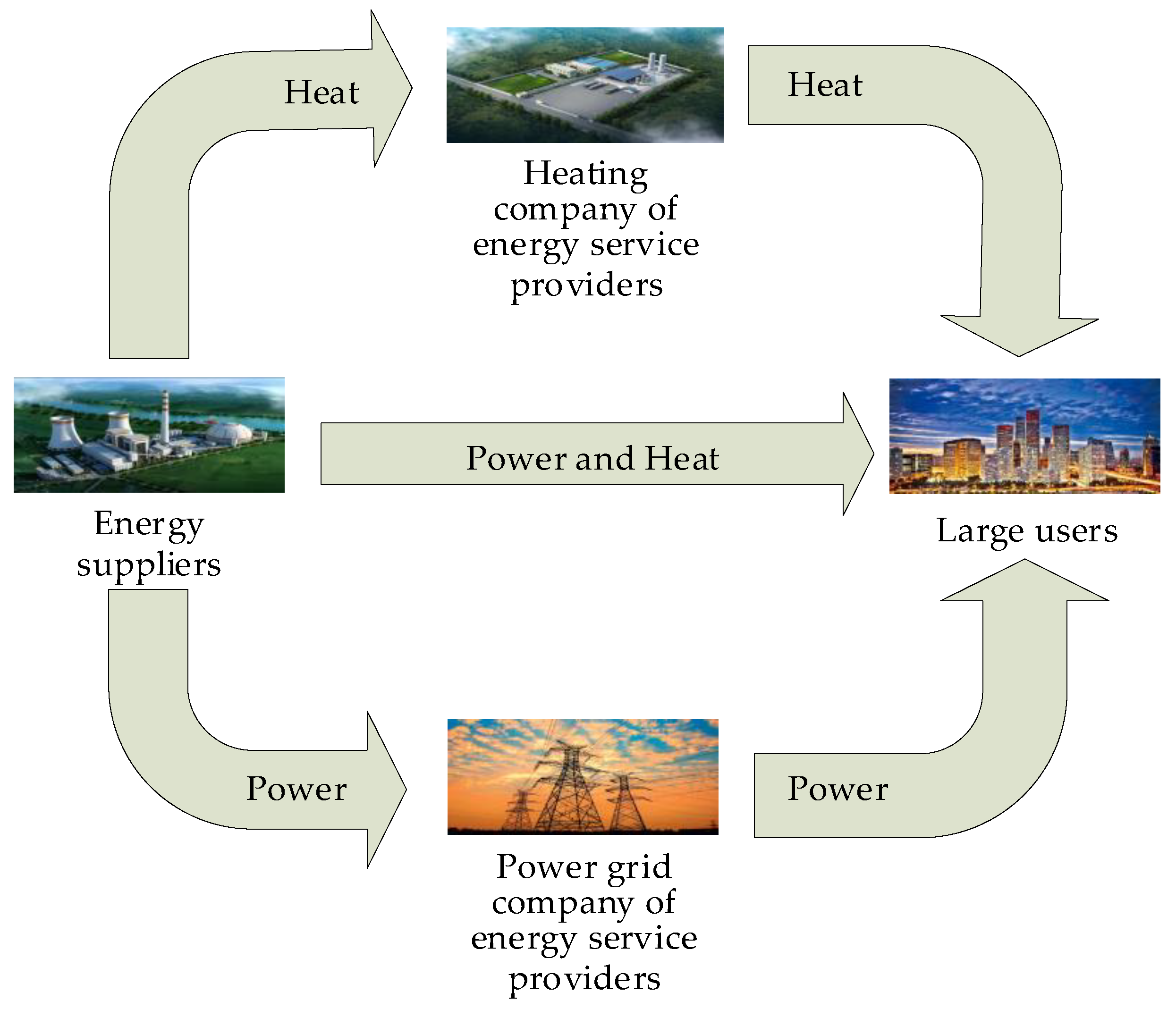
2.1.1. Market Trading Mechanism

The energy market transaction entities of urban energy internet mainly include energy suppliers, energy service providers (including the power grid company and the heating company) and the large users.

The basic market transaction setup is as follows. Large users first forecast the load consumptions based on historical data and other information and then submit load data to energy suppliers, the power grid company and the heating company. Then the energy suppliers, power grid company and heating company make bids to the large users at the same time according to the load demand. Large users then choose the party that needs to pay the least amount for the transaction.

More specifically, (1) the energy suppliers own the thermal power plants, and they are assumed to operate in a typical mode of “fixing heat based on power” to supply energy. Energy suppliers give priority to meeting the thermal needs of large users. At the same time, electricity is sold to the large users or power grid company in the role of energy service provider. (2) The power grid and heating companies purchase excess electricity and heat from energy suppliers and then sell electricity and heat to large users. (3) Large users can choose to purchase heat and electricity from energy suppliers and pay service fees to energy service providers at the same time, or directly purchase electricity from the power grid and then convert part of the electricity into heat energy through electric heating equipment, or purchase heat and electricity separately from the heating company and power grid company.

The structure of the transactions in the urban energy internet market is shown in Figure 1.

From the perspective of large users, how to maximize their benefits when purchasing heat and power has become the focus of the energy internet market. Faced with the quotations of energy service providers and energy suppliers, large users are likely to choose the transaction mode with the maximum revenue. In this paper, we introduce game theory to analyze the trading behavior of various market participants, as well as the transactions realized with other market participants in the urban energy internet.

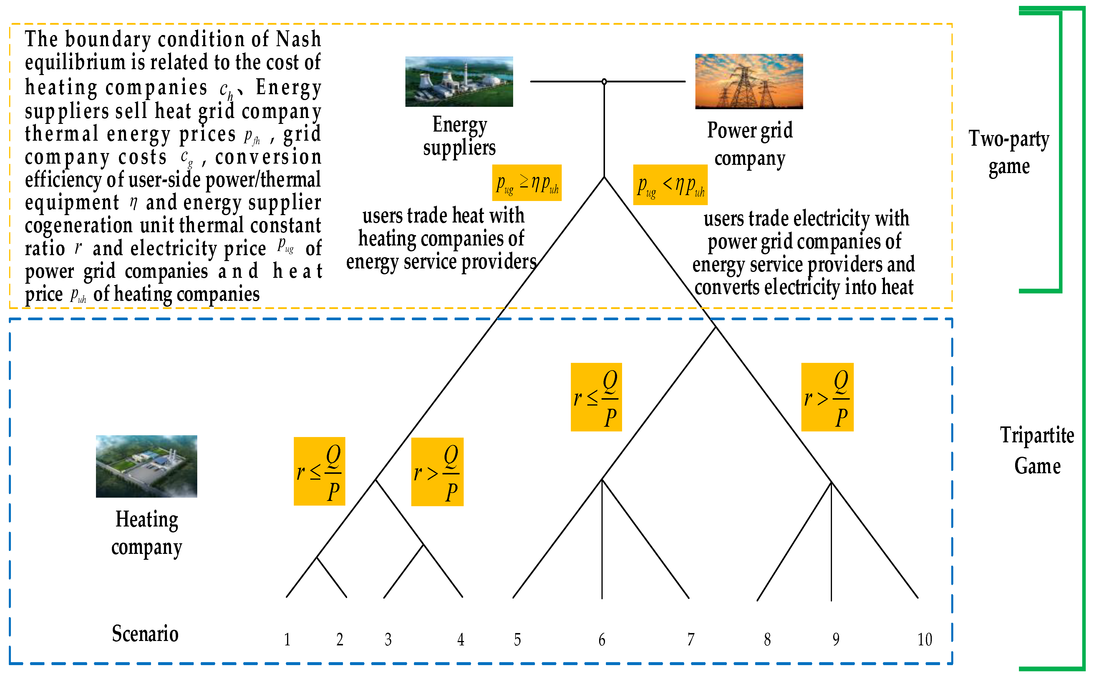
2.1.2. Tripartite Game Model

Before establishing the game model, several assumptions should be clarified. (1) All participants are completely rational, and the game participants in the urban energy internet market, namely the energy suppliers, the large users and energy service providers, act independently under the market trading mechanism. (2) Within a short period of time, the energy consumption, or power and heat generation, of the participants do not change. (3) Only the impact of price and the amounts of electricity and heat are considered in the process of trading; other market factors that affect the trading behavior are neglected.

Therefore, in this non-cooperative static game with complete information, the general tripartite game model can be expressed as:

$$T=\langle N,S,u\rangle$$

(1)

The model contains three elements:

(1)

Game entities $N$: energy internet market entities include all of the energy suppliers $F_j$,$\forall j\in \left\{1,2,\dots M\right\}$, energy service providers of both power grid companies $G$ and heating companies $H$, and the large users $U$.

(2)

Game strategies $S$: in the energy internet market, the game strategy of each participant is its quotation price.

(3)

Game utilities $u$: every rational participant wants to make a deal and get a payoff under the Nash equilibrium.

2.2. Market Entities’ Cost–Income Model

The game payoff function for each player in the market can be shown as [27]:

$$\{\begin{array}{c}{u}_F=u_{Ftra}+u_{Fser}+u_{Foth}\\ u_G=u_{Gtra}+u_{Gser}+u_{Goth}\\ u_H=u_{Htra}+u_{Hser}+u_{Hoth}\\ u_U=u_{Utra}+u_{User}+u_{Uoth}\end{array}$$

(2)

where $u_F$,$u_G$,$u_H$ and $u_U$ denote the game payoffs of energy suppliers, power grid company, heating company, and the large user, respectively; $u_{Ftra}$, $u_{Gtra}$, $u_{Htra}$ and $u_{Utra}$ mean the transaction revenues of energy suppliers, power grid company, heating company and the large user, respectively; $u_{Fser}$, $u_{Gser}$, $u_{Hser}$ and $u_{User}$ mean the service fees of energy suppliers, power grid company, heating company and the large user, respectively; $u_{Foth}$, $u_{Goth}$, $u_{Hoth}$ and $u_{Uoth}$ mean the other benefits of energy suppliers, power grid company, heating company and the large user, respectively.

2.2.1. Energy Suppliers

(a)

Transaction revenue function $u_{Ftra}$: For each energy supplier $F_j$,$\forall j\in \left\{1,2,\dots M\right\}$, its transaction revenue by trading electricity and heat can be represented as

$$u_{Ftra}={\displaystyle \sum }_{j=1}^M{Q}_{fj}{p}_{fqj}+{\displaystyle \sum }_{j=1}^M{P}_{fj}{p}_{fcj}+{\displaystyle \sum }_{j=1}^M{P}_{fgj}{p}_{fg}+{\displaystyle \sum }_{j=1}^M{Q}_{fhj}{p}_{fh}$$

(3)

where $M$ is the number of energy suppliers; $Q_{fj}$ and $p_{fqj}$ represent, respectively, the amount of heat and its price that the $j$-th energy supplier trades with the large user; $P_{fj}$ and $p_{fcj}$ mean the amount of electricity and its price that the $j$-th energy supplier trades with large user, respectively; $P_{fgj}$ and $p_{fg}$ mean the amount of heat and its price, respectively, that the $j$-th energy supplier trades with power grid company; $Q_{fhj}$ and $p_{fh}$ mean the amount of heat and its price, respectively that the $j$-th energy supplier trades with the heating company.

(b)

Service fee function $u_{Fser}$: Energy service providers charge service fees for transactions between energy suppliers and large user:

$$u_{Fser}=-{\displaystyle \sum }_{j=1}^M{P}_{fj}{p}_{ser}-{\displaystyle \sum }_{j=1}^M{Q}_{fj}{p}_{hser}$$

(4)

where $p_{ser}$ is the electricity service fee charged by the power grid company when the energy suppliers trade electricity directly with the large user and $p_{hser}$ is the heat service fee charged by the heating company when the energy suppliers trade heat directly with the large user.

(c)

Other benefit function $u_{Foth}$: other benefits of energy suppliers are expressed only at cost. In order to show the relationship between energy suppliers’ electricity and heat energy transactions and their respective costs, the electricity and heat energy costs are calculated separately in the cost model. Therefore, other benefit of energy suppliers can be expressed as

$$u_{Foth}=-{\displaystyle \sum }_{j=1}^M{P}_f{c}_f-{\displaystyle \sum }_{j=1}^M{Q}_f{q}_f$$

(5)

where $P_f$ and $c_f$ are the power generation amount and unit power generation cost of the $j$-th energy supplier and $Q_f$ and $q_f$ are the heat production amount and unit heat production cost of the $j$-th energy supplier.

The three types of game revenues of the $j$-th energy supplier can be combined as:

$$\begin{array}{ll}{u}_F& =u_{Ftra}+u_{Fser}+u_{Foth}\\ & =({\displaystyle \sum _{j=1}^M{Q}_{fj}}{p}_{fqj}+{\displaystyle \sum _{j=1}^M{P}_{fj}}{p}_{fcj}+{\displaystyle \sum _{j=1}^M{P}_{fgj}}{p}_{fg}+{\displaystyle \sum _{j=1}^M{P}_{fhj}}{p}_{fh}-{\displaystyle \sum _{j=1}^M{P}_{fj}}{p}_{ser}-{\displaystyle \sum _{j=1}^M{Q}_{fj}}{p}_{hser}-{\displaystyle \sum _{j=1}^M{P}_f}{c}_f-{\displaystyle \sum _{j=1}^M{Q}_f}{q}_f)\end{array}$$

(6)

2.2.2. Large User

Without loss of generality, the large users in the urban energy internet are considered as one load aggregator to participate in the energy market.

(a)

Transaction revenue function $u_{Utra}$: $u_{Utra}$ can be formulated as

$$u_{Utra}=-{\displaystyle \sum }_{j=1}^M{Q}_{fj}{p}_{fqj}-{\displaystyle \sum }_{j=1}^M{P}_{fj}{p}_{fcj}-P_{ug}{p}_{ug}-Q_{uh}{p}_{uh}$$

(7)

where $P_{ug}$ and $p_{ug}$ represent the amount of electricity and its price that the power grid company trades with the large, user as an energy service provider, and $Q_{uh}$ and $p_{uh}$ represent the amount of heat and its price that the heating company trades with the large user, as an energy service provider.

(b)

Service fee function $u_{User}$: $u_{User}$ can be formulated as:

$$u_{User}=-{\displaystyle \sum }_{j=1}^M{P}_{fj}{p}_{ser}-{\displaystyle \sum }_{j=1}^M{Q}_{fj}{p}_{hser}$$

(8)

(c)

Other benefit function $u_{Uoth}$: large users have no other benefits, which is assumed to be $u_{Uoth}=0$, since the large user can use electric heating equipment to convert electrical energy bought from the grid company into heat so as to meet the heat demand.

The game payoff of the large user can be combined as

$$\begin{array}{ll}{u}_U& =u_{Utra}+u_{User}+u_{Uoth}\\ & =-{\displaystyle \sum _{j=1}^M{Q}_{fj}}{p}_{fqj}-{\displaystyle \sum _{j=1}^M{P}_{fj}}{p}_{fcj}-P_{ug}{p}_{ug}-Q_{uh}{p}_{uh}-{\displaystyle \sum _{j=1}^M{P}_{fj}}{p}_{ser}-{\displaystyle \sum _{j=1}^M{Q}_{fj}}{p}_{hser}\end{array}$$

(9)

2.2.3. Power Grid Company as an Energy Service Provider

(a)

Transaction revenue function $u_{Gtra}$:

$$u_{Gtra}=-{\displaystyle \sum }_{j=1}^M{P}_{fgj}{p}_{fg}+P_{ug}{p}_{ug}$$

(10)

(b)

Service fee $u_{Gser}$:

$$u_{Gser}=2{\displaystyle \sum }_{j=1}^M{P}_{fj}{p}_{ser}$$

(11)

(c)

Other benefit $u_{Goth}$: Other benefits for the power grid company as an energy service provider are only related to its own costs:

$$u_{Goth}={\displaystyle \sum }_{j=1}^M{P}_{fgj}{c}_g-P_{ug}{c}_g$$

(12)

where $c_g$ is the unit cost of electricity sold by the power grid company.

The game payoffs of the power grid company as an energy service provider can be combined into

$$\begin{array}{ll}{u}_G& =u_{Gtra}+u_{Gser}+u_{Goth}\\ & =-{\displaystyle \sum _{j=1}^M{P}_{fgj}}{p}_{fg}+P_{ug}{p}_{ug}+2{\displaystyle \sum _{j=1}^M{P}_{fj}}{p}_{ser}+{\displaystyle \sum _{j=1}^M{P}_{fgj}}{c}_g-P_{ug}{c}_g\end{array}$$

(13)

2.2.4. Heating company as an energy service provider

(a)

Transaction revenue $u_{Htra}$:

$$u_{Htra}=-{\displaystyle \sum }_{j=1}^M{Q}_{fhj}{p}_{fh}+Q_{uh}{p}_{uh}$$

(14)

(b)

Service fee function $u_{Hser}$:

$$u_{Hser}=2{\displaystyle \sum }_{j=1}^M{Q}_{fj}{p}_{hser}$$

(15)

(c)

Other benefit function $u_{Hoth}$. Other benefits for the heating company as an energy service provider are only related to its own costs:

$$u_{Hoth}={\displaystyle \sum }_{j=1}^M{Q}_{fhj}{c}_h-Q_{uh}{c}_h$$

(16)

where $c_h$ is the unit cost of heat sold by the heating company.

The game payoffs of the heating company as an energy service provider can be combined into

$$\begin{array}{ll}{u}_H& =u_{Htra}+u_{Hser}+u_{Hoth}\\ & =-{\displaystyle \sum _{j=1}^M{Q}_{fhj}}{p}_{fh}+Q_{uh}{p}_{uh}+2{\displaystyle \sum _{j=1}^M{Q}_{fj}}{p}_{hser}+{\displaystyle \sum _{j=1}^M{Q}_{fhj}}{c}_h-Q_{uh}{c}_h\end{array}$$

(17)

Therefore, in the urban energy internet market, the strategy of the energy suppliers is the electricity price $p_{fcj}$, and the strategies of the energy service providers are the service fees $p_{ser}$ and $p_{hser}$. According to the trading mechanism in Section 2.1.1, the large users choose to trade with the party that needs to pay the least amount based on their payoff functions. In other words, the large users do not need to participate directly with a specific strategy; thus, there will be only three game players out of the four market entities in our game model, which is then named as a tripartite game model. The strategy sets of the three game players are $\left[0,p_{fcj}^{max}\right],\forall j\in \left\{1,2,\dots M\right\}$, $\left[0,p_{ser}^{max}\right]$ and $\left[0,p_{hser}^{max}\right]$, respectively. $p_{fcj}^{max}$, $p_{ser}^{max}$ and $p_{ser}^{max}$ are the upper limits of strategies for the three game players, respectively.

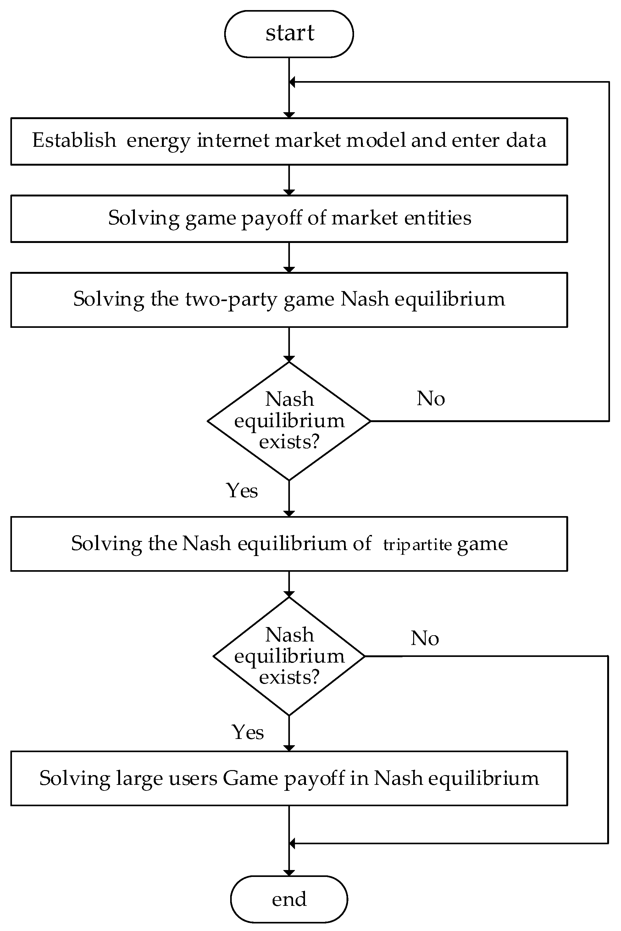
2.3. A New Nash Equilibrium Solving Method for the Tripartite Game Model

At present, there are many methods to solve the Nash equilibria in game problems. Traditional methods include the scribing method, definition method, iterative search method and method of eliminating unfavorable strategy sets [28]. In addition, there are some special Nash equilibrium solutions, such as the Lemke method for constrained affine generalized Nash equilibrium problem [29], the augmented Lagrangian method for generalized Nash equilibrium problems [30] and multi-Nash equilibrium solution algorithm based on learning theory. The game problem in this paper is solved by searching the entire strategy space, according to the definition of Nash equilibrium [31,32,33].

In the tripartite game model of energy internet market, the game payoffs of the energy suppliers are related to different strategy combinations of $p_{fcj}$, $p_{ser}$ and $p_{hser}$ of all game players. The game payoff of the power grid company as an energy service provider is related to two game players’ strategies of $p_{fcj}$ and $p_{ser}$. However, the game payoff of the heating company as an energy service provider is only related to its own strategy of $p_{hser}$.

Therefore, we propose a new game-tree search method for the tripartite game model. The tree-diagram of the Nash equilibria solution for the tripartite game is shown in Figure 2, and the detailed solution process is described as follows.

(1) Firstly, the existence of the Nash equilibria for the proposed tripartite game on the continuous strategy sets is demonstrated.

According to Nash’s Existence Theorem, any n-player normal-form game with finite strategy sets for all players has a Nash equilibrium in mixed strategies [31,32,33]. Therefore, the Nash equilibria of the proposed tripartite game model will surely exist, due to the fact that the strategies of all three game players in the urban energy internet belong to mix strategies with finite value space.

In this game problem, the strategies for game players to participate in market competition are all continuous variables. The Nash equilibrium problem of continuous strategy game can be solved by analyzing the specific participant’s best response function to other participants’ strategy combinations. It can be seen from Section 2.2 that the game players’ payoff functions are typically piecewise linear functions, so the best response function of each participant can be considered in segments, and the Nash equilibria of the game can be obtained by combining the segmented results together.

Since the payoff functions are not continuous, the conventional iterative search methods are not applicable. Therefore, the proposed tripartite game problem can be solved by searching the entire strategy space, according to the definition of Nash equilibrium. To solve the game model on a computer platform, it is necessary to discretize the game players’ strategies. The formulas are as follows:

$$\{\begin{array}{l}{p}_{fcj}^{max}=k_j\ast p_{fcj}^{step},k_j\in {\mathbb{Z}}^{+},\forall j\in \left\{1,2,\dots M\right\}\\ p_{ser}^{max}=k_0\ast p_{ser}^{step},k_0\in {\mathbb{Z}}^{+}\end{array}$$

(18)

where, for the energy supplier, the lower limit of its strategy $p_{fcj}$ is 0 and the upper limit is $p_{fcj}^{max}$, with an incremental step size of $p_{fcj}^{step}$ and a total number of $k_j$ steps; for the grid company, its strategy has a lower limit of 0 and upper limit of $p_{ser}^{max}$, with an incremental step size of $p_{ser}^{step}$ and a total number of $k_0$ steps. According to Nash’s existence theorem [31,32,33], there is a Nash equilibrium solution for a game problem with finite strategy sets after discretization.

(2) Then, the Nash equilibria of the two-party game model can be obtained by searching the best payoffs of the two participants [31].

Since the game payoff of the heating company as an energy service provider is only related to its own strategy $p_{hser}$, we can reformulate the best response functions for the energy supplier and power grid company based on piecewise functions according to the variable $p_{hser}$. Then, the proposed tripartite game model can be simplified to a two-party game problem for each value of $p_{hser}$.

For the mixed strategy game problem, define ${\sigma }_i^{*}$ as the Nash equilibrium point of a game model; then, the following inequality condition holds:

$$u_i\left({\sigma }_i^{*},{\sigma }_{-i}^{*}\right)\ge u_i\left(s_i,{\sigma }_{-i}^{*}\right),\forall s_i\in S_i,\forall i$$

(19)

where $i$ is the number of game players; $u_i$ is the payoff of the game player $i$; $s_i$ is the strategy of the game player $i$; $S_i$ is the strategy set of the game player $i$; and ${\sigma }_{-i}^{*}$ is strategy combination for the game players other than the player $i$.

Considering the value range of the strategy $p_{hser}$ of the heating company as an energy service provider, the optimal game payoff of the heating company can be reached under the Nash equilibrium constraint of the two-party game problem in each branch search scenario of the game tree.

(3) Lastly, through the above game-tree search method, the Nash equilibria of the tripartite game can be solved, and the flowchart for the solving process is shown in Figure 3.

3. Results

In order to verify the effectiveness of the tripartite game model and the solving method for the urban energy internet market, case studies are conducted as follows. The thermal load demand of the large user is $Q$, the electrical load demand is $P$, the thermoelectric ratio of energy supplier is $r$ and the electrical–heat conversion efficiency of large user is $\eta$. The basic system parameters are described in

Table 1. Energy internet parameters. (Note that there is only one energy supplier in this section, namely $j=1$; $p_{fcj}$ is thus simplified to $p_{fc}$.)

Parameters	Values (unit)	Parameters	Values (unit)
$Q$	3 MW	$P$	5 MW
$c_f$	0.5 yuan/(kW·h)	$c_g$	0.6 yuan/(kW·h)
$c_h$	0.5 yuan/(kW·h)	$\eta$	0.9
$p_{fg}$	0.2 yuan /(kW·h)	$p_{fh}$	0.2 yuan/(kW·h)
$p_{ug}$	1.2 yuan/(kW·h)	$p_{uh}$	0.8 yuan/(kW·h)
$p_{fqj}$	0.8 yuan/(kW·h)	$p_{fc}$	$p_{fc}\in \left[0,2\right]$ yuan/(kW·h)
$p_{ser}$	$p_{ser}\in \left[0,1.5\right]$ yuan /(kW·h)	$p_{hser}$	$p_{hser}\in \left[0,1\right]$ yuan/(kW·h)

. The solution program is coded on the MATLAB platform to solve Nash equilibria of the tripartite game model, and the graphic result is shown in Figure 4.

It can be seen from Figure 4 that the thermoelectric ratio of energy supplier $r$ and other parameters will affect the transaction objects for the large user.

If $r\le Q/P$, the large user has three bidding options: (1) large user trades both heat and electricity only with the energy supplier; (2) large user purchases electricity from the power grid company, and the energy supplier trades electricity with the power grid company and heat with the heating company; and (3) large user trades electricity with the power grid company and heat with the heating company, and the energy supplier trades electricity with the power grid company and heat with the heating company.

If $r>Q/P$, the energy supplier can provide thermal energy to meet the heat demand of the large user, while the produced electrical energy cannot meet the electricity demand of the large user. Under this condition, the large user needs to purchase additional electrical power from the power grid company.

The Nash equilibria critical condition of the tripartite game model can be obtained by analyzing the strategy variable of the heating company $p_{\mathrm{hser}}$. Considering the heating company’s strategy $p_{\mathrm{hser}}$ and other parameters, the Nash equilibria of the two-party game are shown in Figure 5. There are two types of transactions: one is between the large user and energy supplier; the other is between the large user and energy service providers. The latter includes two scenarios according to the numerical relationship between $p_{ug}$ and $\eta p_{uh}$. The large user will only trade with the power grid company when $p_{ug}\le \eta p_{uh}$. For $p_{ug}>\eta p_{uh}$, the large user will only trade with the heating company. In Figure 5, the line segment part represents the Nash equilibria of transactions between the large user and energy supplier. The rectangular area represents the Nash equilibria of transactions between the large user and energy service providers.

More specifically, when $p_{ug}\ge \eta p_{uh}$, the tripartite game Nash equilibria change with the strategy $p_{hser}$ of the third party. As $p_{hser}$ goes from 0 to its maximum, the line segment $A_1{A}_2$ will merge to the point $A_3$, and the Nash equilibria critical point of the transaction between the large user and energy supplier will be $A_3$, and the following equation will be satisfied: $p_{hser}=\frac{1}{2}\left(p_{uh}-p_{fh}\right)$ for the third-party strategy variable. Beyond this critical point, the line segment part disappears, and the large user is better off choosing to trade with the energy supplier.

When $p_{ug}<\eta p_{uh}$, similarly, the line segment $A_1{A}_2$ will merge to the point $A_3$, and the following equation will be satisfied: $p_{hser}=\frac{1}{2}\left(c_g/\eta -p_{fh}\right)$ for the third party strategy variable.

The parameters of electrothermal conversion efficiency $\eta$, thermoelectric ratio $r$, the heat and electricity costs $c_h$ and $c_g$ of energy service providers, the electricity price $p_{ug}$ of power grid companies and heat price $p_{uh}$ of heating companies, will affect the Nash equilibria distribution of the tripartite game. The simulation results of the tripartite game model include 10 scenarios. The analysis is carried out under the most complex Nash equilibria correspondence condition for one scenario under the condition of $p_{ug}\le \eta p_{uh}$, $r\le \frac{Q}{P}$ and $\frac{c_g}{\eta }>c_h>\frac{c_g/\eta +p_{fh}}{2}$; the details of the Nash equilibria regions are shown in Figure 6. Other scenarios are supplemented in Appendix A.

The Nash equilibria of the tripartite game will satisfy the expressions shown in (20) in this scenario, which can be further divided into four intervals.

$$\{\begin{array}{ll}{p}_{ser}>\frac{p_{ug}-p_{fg}+r\left(\frac{p_{ug}}{\eta }-p_{fh}-2p_{hser}\right)}{2},p_{fc}>\frac{p_{ug}+p_{fg}}{2}+\frac{r\left(p_{ug}+c_g\right)}{2\eta }-r\left(p_{fqj}+p_{hser}\right)& \frac{c_h-p_{fh}}{2}>p_{hser}\\ p_{ser}+p_{fc}=p_{ug}+r\frac{p_{ug}}{\eta }-r\left(p_{fqj}+p_{hser}\right){,}_{ser}>\frac{p_{ug}-p_{fg}+r\left(\frac{p_{ug}}{\eta }-p_{fh}-2p_{hser}\right)}{2},p_{fc}>\frac{p_{ug}+p_{fg}}{2}+\frac{r\left(p_{ug}+c_g\right)}{2\eta }-r\left(p_{fqj}+p_{hser}\right)& \frac{c_h+\frac{c_g}{\eta }-2p_{fh}}{4}>p_{hser}>\frac{c_h-p_{fh}}{2}\\ p_{ser}+p_{fc}=p_{ug}+r\frac{p_{ug}}{\eta }-r\left(p_{fqj}+p_{hser}\right),p_{ser}+p_{fc}\ge p_{ug}+r\frac{p_{ug}}{\eta }-r\left(p_{fqj}+\frac{c_h-p_{fh}}{2}\right),p_{ser}>\frac{p_{ug}-p_{fg}+r\left(\frac{p_{ug}}{\eta }-p_{fh}-2p_{hser}\right)}{2},p_{fc}>\frac{p_{ug}+p_{fg}}{2}+\frac{r\left(p_{ug}+c_g\right)}{2\eta }-r\left(p_{fqj}+p_{hser}\right)& \frac{\frac{c_g}{\eta }-p_{fh}}{2}\ge p_{hser}\ge \frac{c_h+\frac{c_g}{\eta }-2p_{fh}}{4}\\ p_{ser}+p_{fc}\ge p_{ug}+r\frac{p_{ug}}{\eta }-r\left(p_{fqj}+\frac{c_h-p_{fh}}{2}\right),p_{ser}>\frac{p_{ug}-p_{fg}+r\left(\frac{p_{ug}}{\eta }-p_{fh}-2p_{hser}\right)}{2},p_{fc}>\frac{p_{ug}+p_{fg}}{2}+\frac{r\left(p_{ug}+c_g\right)}{2\eta }-r\left(p_{fqj}+p_{hser}\right)& \frac{p_{ug}}{r}+\frac{p_{ug}}{\eta }-p_{fqj}>p_{hser}>\frac{\frac{c_g}{\eta }-p_{fh}}{2}\end{array}$$

(20)

In Figure 6, the boundary line segment between the large user’s transaction with the energy supplier and the energy service providers is $p_{ser}+p_{fc}=p_{ug}+r\frac{p_{ug}}{\eta }-r\left(p_{fqj}+p_{hser}\right)$, namely the line segment $A_1{A}_2$ in Figure 5.

The trading modes for the four intervals can be expressed as follows.

(1) When $\frac{c_h-p_{fh}}{2}>p_{hser}>0$, the heating company will not have a dominant strategy no matter what strategy $p_{hser}$ is under this scenario, and the line segment of the Nash equilibria part will disappear. The Nash equilibria will only contain the black shaded rectangular region in Figure 6, and the transaction will be realized between the large user and the power grid company. The results can also be derived by the first expression in (20).

(2) When $\frac{c_h+c_g/\eta -2p_{fh}}{4}>p_{hser}>\frac{c_h-p_{fh}}{2}$, the red line segment of the Nash equilibria part represents the transaction between the large user and the energy supplier; the red shaded rectangular region of the Nash equilibria represents the transaction between the large user and the power grid company, or the transaction between the large user and the heating company.

(3) When $\frac{c_g/\eta -p_{fh}}{2}>p_{hser}>\frac{c_h+c_g/\eta -2p_{fh}}{4}$, the blue line segment of the Nash equilibria part also represents the transaction between the large user and the energy supplier; the blue shaded region of the Nash equilibria shows that the transaction will only be realized between the large user and the power grid company in this case.

(4) When $p_{ug}\left(\frac{P}{Q}+\frac{1}{\eta }\right)-P_{fqj}>p_{hser}>\frac{c_g/\eta -p_{fh}}{2}$, the green shaded region of the Nash equilibria represents the transaction between the large user and the power grid company only.

The detailed strategy combination and game payoffs for the market participants in the above scenario are shown in

Table 2. Strategy combination and game payoffs for the market participants in the above scenario.

Variables	User Trading Mode	Strategy Combination	Large User (yuan)	Energy Supplier (yuan)	Power Grid Company (yuan)	Heating Company (yuan)
	With the power grid company	Equilibrium strategy 0 $\left(p_{fc},p_{ser},p_{hser}\right)=\left(0.3,0.3,0.1\right)$	−5000	0	2000	900
Energy supplier’s $p_{fc}$	With the heating company	Non-equilibrium strategy 1 $\left(p_{fc},p_{ser},p_{hser}\right)=\left(0.1,0.3,0.1\right)$	−4700	-500	3000	600
	With the power grid company	Equilibrium strategy 2 $\left(p_{fc},p_{ser},p_{hser}\right)=\left(0.5,0.3,0.1\right)$	−5000	0	2000	900
Power grid company’s $p_{ser}$	With the heating company	Non-equilibrium strategy 3 $\left(p_{fc},p_{ser},p_{hser}\right)=\left(0.3,0.1,0.1\right)$	−4700	500	1000	600
	With the power grid company	Equilibrium strategy 4 $\left(p_{fc},p_{ser},p_{hser}\right)=\left(0.3,0.5,0.1\right)$	−5000	0	2000	900
Heating company’s $p_{hser}$	With the power grid company	Equilibrium strategy 5 $\left(p_{fc},p_{ser},p_{hser}\right)=(0.3,0.3,0.05)$	−5000	0	2000	900
	With the power grid company	Equilibrium strategy 6 $\left(p_{fc},p_{ser},p_{hser}\right)=\left(0.3,0.3,0.2\right)$	−5000	0	2000	900

. It is worth noting that the Nash equilibrium is a continuous region and therefore contains multiple consecutive points related to different game strategy combinations. According to the market trading mechanism in Section 2.1.1, each game player will change its own strategy and choose the trading mode that maximizes its own revenue. For example, there will be two kinds of trading outcomes for the strategy combinations 1 and 2 when changing the energy supplier’s $p_{fc}$. Although the revenue of the power grid company may increase from 2000 to 3000 yuan under the non-equilibrium strategy combination 1, the energy suppliers will not choose strategy 1 because its revenue will decrease from 0 to -500 yuan in that case. Similarly, the power grid company will not choose strategy 3 with revenue as low as 1000 yuan, and the heating company will not choose both strategy 1 and strategy 3, which bring itself the revenue of only 600 yuan. In other words, the game players compare their own income changes when choosing their own strategies, and avoid choosing their strictly disadvantaged strategies. Therefore, the proposed non-cooperative static tripartite game model will make all the market participants more rational.

4. Discussion

The results of the game model established in this study are the Nash equilibrium payoffs of all market participants, including the large user. The market transaction status of the Nash equilibrium state is that under the current market parameters and all possible strategies of other market participants, each market player’s equilibrium strategy or best response tends to maximize its benefits or avoid greater losses. This best response is not the global optimal solution in the optimization theory. Sometimes, if a game player wants to choose the strategy to maximize its benefits, other players will definitely choose an anti-strategy to make it lose more.

In addition, the proposed energy market trading model was initially proposed for the urban energy internet. Typically, in a town/urban area, there may be only one energy service provider who owns the transmission/distribution power network and another one who owns the heat supply pipeline network. It is also assumed that the users do not participate in the market as demand response service providers. As for the energy suppliers, they usually have similar payoff functions, according to the revenue and benefit functions in Section 2.2.1. Therefore, the proposed energy market trading model based on tripartite game theory is feasible in practice. Future work can be extended to add some additional market participants, including the demand response service providers, multiple energy service providers (more than two), in order to implement the proposed energy trading model to a larger energy market.

5. Conclusions

There are many key transaction issues that need to be resolved in the energy internet market. A tripartite game model is established to solve the multi-energy joint trading problem and market equilibrium problem in this paper. A game-tree search method for solving the game model based on the Nash equilibrium definition is proposed by analyzing the cost–income function and market transaction mechanism of each market entity. We are able to analyze the market transaction status for the participants based on the corresponding market transactions in different Nash equilibria scenarios and prove the applicability of the tripartite game model for multi-energy joint trading problems. The results show that the established model can effectively realize market equilibria with the best responses for all the market participants in the urban energy internet.

References

1. Huang, A.Q.; Crow, M.L.; Heydt, G.T.; Zheng, J.P.; Dale, S.J. The Future Renewable Electric Energy Delivery and Management (FREEDM) System: The Energy Internet. Proc. IEEE 2011, 99, 133–148. [Google Scholar] [CrossRef]
2. Zhou, K.; Yang, S.; Shao, Z. Energy Internet: The business perspective. Appl. Energy 2016, 178, 212–222. [Google Scholar] [CrossRef]
3. Ma, Z.; Zhou, X.X.; Shang, Y.W.; Sheng, W.X. Exploring the concept, key technologies and development model of energy Internet. Power Syst. Technol. 2015, 39, 3014–3022. [Google Scholar] [CrossRef]
4. Liu, F.; Bie, Z.H.; Liu, S.Y.; Li, G.F. Framework design, transaction mechanism and key issues of Energy Internet Market. Automat. Electr. Power Syst. 2018, 42, 108–117. [Google Scholar] [CrossRef]
5. Lu, Q.; Lü, S.; Leng, Y. A Nash-Stackelberg game approach in regional energy market considering users’ integrated demand response. Energy 2019, 175, 456–470. [Google Scholar] [CrossRef]
6. Gabriel, S.A.; Conejo, A.J.; Fuller, J.D.; Hobbs, B.F.; Ruiz, C. Complementarity Modeling in Energy Markets; Springer Science & Business Media: Berlin/Heidelberg, Germany, 2012; p. 1. ISBN 9781441961235. [Google Scholar]
7. Durvasulu, V.; Hansen, T.M. Benefits of a demand response exchange participating in existing bulk-power markets. Energies 2018, 11, 3361. [Google Scholar] [CrossRef] [Green Version]
8. Zhang, C.; Yan, W. Spot market mechanism design for the electricity market in china considering the impact of a contract market. Energies 2019, 12, 1064. [Google Scholar] [CrossRef] [Green Version]
9. Cheng, C.T.; Chen, F.; Li, G.; Tu, Q.T. Market equilibrium and impact of market mechanism parameters on the electricity price in Yunnan’s electricity market. Energies 2016, 9, 463. [Google Scholar] [CrossRef] [Green Version]
10. Wang, C.; Wei, W.; Wang, J.; Liu, F.; Mei, S. Strategic offering and equilibrium in coupled gas and electricity markets. IEEE Trans. Power Syst. 2017, 33, 290–306. [Google Scholar] [CrossRef]
11. Chen, R.Z.; Wang, J.H.; Sun, H.B. Clearing and pricing for coordinated gas and electricity day-ahead markets considering wind power uncertainty. IEEE Trans. Power Syst. 2018, 33, 2496–2508. [Google Scholar] [CrossRef]
12. Zhao, S.N.; Wang, B.B.; Li, Y.C.; Li, Y. Integrated energy transaction mechanisms based on blockchain technology. Energies 2018, 11, 2412. [Google Scholar] [CrossRef] [Green Version]
13. Fudenberg, D.; Levine, D.K. The Theory of Learning in Games; MIT Press Books: Cambridge, MA, USA, 1998; p. 1. ISBN 9780262061940. [Google Scholar]
14. Zhao, N.; Xia, T.; Yu, T.; Liu, C. Subsidy-related deception behavior in energy-saving products based on game theory. Front. Energy Res. 2020, 7, 1–10. [Google Scholar] [CrossRef] [Green Version]
15. Von Neumann, J.; Morgenstern, O.; Kuhn, H.W. Theory of Games and Economic Behavior (Commemorative Edition); Princeton University Press: Princeton, NJ, USA, 2007; p. 1. ISBN 9781400829460. [Google Scholar]
16. Saad, W.; Zhu, H.; Poor, H.V. Coalitional game theory for cooperative micro-grid distribution networks. In Proceedings of the 2011 IEEE International Conference on Communications Workshops (ICC), Kyoto, Japan, 5–9 June 2011; pp. 1–5. [Google Scholar]
17. Kasbekar, G.S.; Sarkar, S. Pricing games among interconnected microgrids. In Proceedings of the 2012 IEEE Power and Energy Society General Meeting (PESGM), San Diego, CA, USA, 22–26 July 2012; pp. 1–8. [Google Scholar]
18. Mohsenian-Rad, A.H.; Wong, V.W.S.; Jatskevich, J.; Schober, R.; Leon-Garcia, A. Autonomous demand-side management based on game-theoretic energy consumption scheduling for the future smart grid. IEEE Trans. Smart Grid 2010, 1, 320–331. [Google Scholar] [CrossRef] [Green Version]
19. Han, X.J.; Wang, F.; Tian, C.G.; Xue, K.; Zhang, J.F. Economic evaluation of actively consuming wind power for an integrated energy system based on game theory. Energies 2018, 11, 1476. [Google Scholar] [CrossRef] [Green Version]
20. Zang, T.; Xiang, Y.; Yang, J. The tripartite game model for electricity pricing in consideration of the power quality. Energies 2017, 10, 2025. [Google Scholar] [CrossRef] [Green Version]
21. Gao, B.T.; Zhang, W.H.; Tang, Y.; Hu, M.J.; Zhu, M.C.; Zhan, H.Y. Game-theoretic energy management for residential users with dischargeable plug-in electric vehicles. Energies 2014, 7, 7499–7518. [Google Scholar] [CrossRef]
22. Karavas, C.S.; Arvanitis, K.; Papadakis, G. A game theory approach to multi-agent decentralized energy management of autonomous polygeneration microgrids. Energies 2017, 10, 1756. [Google Scholar] [CrossRef] [Green Version]
23. Dong, F.G.; Ding, X.H.; Shi, L. Wind power pricing game strategy under the china’s market trading mechanism. Energies 2019, 12, 3456. [Google Scholar] [CrossRef] [Green Version]
24. He, Y.X.; Song, D.; Xia, T.; Li, W.Y. Mode of generation right trade between renewable energy and conventional energy based on cooperative game theory. Power Syst. Technol. 2017, 41, 2485–2490. [Google Scholar] [CrossRef]
25. Yang, Z.; Peng, S.C.; Liao, Q.F.; Liu, D.C.; Xu, Y.Y.; Zhang, Y.J. Non-cooperative trading method for three market entities in integrated community energy system. Automat. Electr. Power Syst. 2018, 42, 32–39. [Google Scholar] [CrossRef]
26. Fang, Y.J.; Chen, L.J.; Mei, S.W.; Huang, S.W. Marketing equilibria of integrated heating and power system considering locational marginal pricing in distribution networks. J. Eng. 2017, 14, 2609–2614. [Google Scholar] [CrossRef]
27. Liu, J.; Wang, C.; Chen, J.C.; Liu, X.M.; Liu, Y.W. Game theory based profit model for multiple market entities of urban energy internet. Automat. Electr. Power Syst. 2019, 43, 90–96. [Google Scholar] [CrossRef]
28. Ma, Z.; Callaway, D.S.; Hiskens, I.A. Decentralized charging control of large populations of plug-in electric vehicles. IEEE Trans. Control Syst. Technol. 2012, 21, 67–78. [Google Scholar] [CrossRef]
29. Kanzow, C.; Steck, D. Augmented Lagrangian methods for the solution of generalized Nash equilibrium problems. SIAM J. Optim. 2018, 26, 2034–2058. [Google Scholar] [CrossRef] [Green Version]
30. Schiro, D.A.; Pang, J.S.; Shanbhag, U.V. On the solution of affine generalized Nash equilibrium problems with shared constraints by Lemke’s method. Math. Program. 2013, 142, 1–46. [Google Scholar] [CrossRef]
31. Mei, S.W. The Basis of Engineering Game Theory and its Power System Application; China Science Press: Beijing, China, 2016; p. 1. ISBN 9787030500106. [Google Scholar]
32. Gibbons, R. Game Theory for Applied Economist; Pricenton University Press: Princeton, NJ, USA, 1992; p. 1. ISBN 9780691003955. [Google Scholar]
33. Luo, Y.F. Game Theory; Tsinghua University Press; Beijing Jiaotong University Press: Beijing, China, 2007; p. 1. ISBN 9787811231052. [Google Scholar]
Figure 1. Energy internet market structure.
Energies 13 01834 g001
Figure 2. Game-tree diagram for the Nash equilibria solution of the tripartite game.
Energies 13 01834 g002
Figure 3. The process of solving Nash equilibria for the proposed tripartite game model.
Energies 13 01834 g003
Figure 4. Nash equilibria of the tripartite game.
Energies 13 01834 g004
Figure 5. Two-party sketch of the game Nash equilibria.
Energies 13 01834 g005
Figure 6. Two-dimensional display of tripartite game Nash equilibria.
Energies 13 01834 g006