Reconstruction of Multidecadal Country-Aggregated Hydro Power Generation in Europe Based on a Random Forest Model

Abstract

Hydro power can provide a source of dispatchable low-carbon electricity and a storage solution in a climate-dependent energy mix with high shares of wind and solar production. Therefore, understanding the effect climate has on hydro power generation is critical to ensure a stable energy supply, particularly at a continental scale. Here, we introduce a framework using climate data to model hydro power generation at the country level based on a machine learning method, the random forest model, to produce a publicly accessible hydro power dataset from 1979 to present for twelve European countries. In addition to producing a consistent European hydro power generation dataset covering the past 40 years, the specific novelty of this approach is to focus on the lagged effect of climate variability on hydro power. Specifically, multiple lagged values of temperature and precipitation are used. Overall, the model shows promising results, with the correlation values ranging between 0.85 and 0.98 for run-of-river and between 0.73 and 0.90 for reservoir-based generation. Compared to the more standard optimal lag approach the normalised mean absolute error reduces by an average of 10.23% and 5.99%, respectively. The model was also implemented over six Italian bidding zones to also test its skill at the sub-country scale. The model performance is only slightly degraded at the bidding zone level, but this also depends on the actual installed capacity, with higher capacities displaying higher performance. The framework and results presented could provide a useful reference for applications such as pan-European (continental) hydro power planning and for system adequacy and extreme events assessments.

1. Introduction

Hydro power is the largest renewable energy resource in Europe, accounting for 325,000 GWh of generation in 2017, equivalent to approximately 42% of EU renewable energy generation or 10.8% of European total net electricity generation [1]. Hydro power, in particular through reservoir-based power plants, plays a critical role in providing flexibility to the European power systems. With the EU renewable energy target of 32% by 2030 [2], the role of hydro power will be even more important in a low-carbon scenario, where the capacity of non-dispatchable electricity sources (mostly wind and solar) will be much higher than today [3].

Like wind and solar power, hydro power is a climate-dependent energy source. To date, its power generation has been mostly modelled by means of physical models with technical parameters specified for individual power plants. There are several explanations for this approach: (i) modelling tends to be thought of as a bottom-up approach, therefore starting from individual power plants (to e.g., assist with their operations) rather than at the entire country or pan-European level; (ii) the impacts of climate variables on hydro power are varied and complex, and many factors contribute to these impacts such as watershed characteristics, the river flow rate, the evaporation process, and human factors, and hence, using only climate data is not sufficient to predict hydro power generation at the desired accuracy for plant-level operational purposes; (iii) hydro power generation at the European level has only recently started to become publicly available (as further discussed below); (iv) the quality of climate data as provided by reanalysis (i.e., climate reconstructions), and particularly precipitation, has been improving significantly only in recent years.

Wind and solar power play an increasingly important role in a low-carbon energy plan. However, their weather-dependent nature requires a more stable energy source, together with storage solutions, to cope with climate variability. Hydro power is a good candidate with its ability to dispatch or store electricity according to demand. For example, [4] showed that integrating run-of-river power with wind and solar power, for 12 European areas, increases the penetration rate of wind and solar power by a few to several percentage points.

Moreover, understanding and predicting hydro power generation at a scale larger than individual power plants could be beneficial to Transmission System Operators (TSOs)—the primary role of which is to ensure the balance of power networks at a large scale. Thus, understanding the impacts of climate variability on hydro power can assist with ensuring a stable pan European electricity network in time. In addition, other specialists such as energy traders require and utilize large-scale power production estimations for their bidding. An accessible homogenous hydro power dataset for Europe over several decades, by extending the short periods (normally a few years) of publicly available power generation data, would therefore provide an invaluable input to pan-European network assessment and planning. This is one of the goals of the Copernicus Climate Change Service (C3S) for the Energy Sector (C3S Energy) [5].

Here, we introduce a dataset of hydro power generation for 12 European countries using a machine learning model, the random forest. While the model we propose is highly simplified and uses only two climate variables (2 metre temperature and precipitation) as predictors, it is capable of reproducing with high accuracy observed power generation data at the country level and at the sub-country level (snow depth was also used for testing purposes as described later, but it is not included in the final model). One of the features of this model is that instead of their instantaneous values (for temperature) or daily accumulated values (for precipitation), we mimic the latency of the system by using their lagged values. The lag time is designed to account for processes which usually take longer than the daily timescale to produce an effect on electricity generation, e.g., snow melting, river run-off and underground water processes. In the case of reservoir-based hydro power production, these relationships are even more complex due to human intervention, which controls electricity demand as well as for other competing uses of water (agricultural, domestic, etc.). In this paper, two methods of lag calculation—optimal lag and multiple lags—are compared to each other and against a baseline model with daily climate values.

Two types of hydro power generation are considered: (i) reservoir-based generation, where water is stored behind a dam to be dispatched when needed; (ii) run-of-river generation, where there is no or minimal storage mechanism. Hydro pump storage was not considered as it contributes only a very small proportion and heavily depends on human management rather than climate conditions. Since energy generation data for specific hydro power plants in Europe are not publicly available, we used the aggregated publicly available data obtained from the European Network of Transmission System Operators for Electricity (ENTSO-E) Transparency Platform [6]. The focus here is mainly at the country level, a large enough spatial scale to cover relevant climate characteristics such as precipitation or snow contributing to hydro power plants. The country average level is also a relevant scale for many applications (European-scale optimisation models for instance), including adequacy outlooks run by TSOs and European-level investments studies. Naturally, however, the countries considered have different sizes, and hence our model provides an indirect measure of its ability to reproduce hydro power generation at different scales. In addition, however, an explicit sub-country test for Italy is also presented.

This paper is structured as follows. Section 2 describes the data used in this work and how the machine learning model was setup. Section 3 shows the model results, including a comparison with measured power data and further validation tests with independent datasets. Finally, Section 4 presents a summary together with a discussion on how to use the model and dataset efficiently.

2. Materials and Methods

2.1. Data

The data used in this work meet two requirements. Firstly, they should be publicly accessible as the C3S Energy service output will be made publicly available; and secondly, they should span a long period and cover as many European countries as possible in a homogenous and consistent manner. Considering these two criteria, we selected European Centre for Medium-Range Weather Forecasts (ECMWF) reanalysis dataset ERA5 (ECMWF Re-Analysis fifth generation) [7] for the climate data and the European Network of Transmission System Operators for Electricity (ENTSO-E) Transparency Platform [6] for the energy data.

The data from the ENTSO-E Transparency Platform includes many variables for different purposes in the energy sector starting from 2015. For this study, we used the Aggregated Generation Per Type product [Product number 16.1.B&C], and specifically reservoir-based and run-of-river hydro power generation. The original data are available at hourly resolution for European countries that report data to ENTSO-E. Since hydro electricity does not normally vary that much at hourly timescales at the country level, we aggregated the data to daily resolution to also reduce computation time. Twelve countries with significant power generation were selected for the study. Their installed capacities are shown in

Table 1. List of 12 countries selected in this study with their country code (ISO 3166) and their installed capacities (in MW) in 2019 (from the European Network of Transmission System Operators for Electricity (ENTSO-E) Transparency Platform, accessed on March 2020).

Country	Country Code	Reservoir	Run of River
Austria	AT	2440	5558
Switzerland	CH	5419	635
Germany	DE	1298	3983
Spain	ES	19,146	1156
Finland	FI	-	3148
France	FR	8279	10,955
Italy	IT	3857	10,650
Norway	NO	27,683	992
Portugal	PT	1515	2858
Romania	RO	3373	2770
Sweden	SE	16,301	-
Slovakia	SK	418	1208

.

As the focus of this study is the impact of climate variability on hydro power generation, we assume that the installed capacity for all countries is constant throughout the training period (2015–2019) as well as the simulated period (1979 to present). In other words, the installed capacity is assumed to be constant over the whole period (1979–2019) because this allows us to isolate and assess the effect of climate variability on hydro power generation. If one were interested in reconstructing the actual hydro power production, this can be achieved by dividing our estimates by the installed capacity (as given in Table 1) and multiplying by the actual installed capacity. Attention is also drawn to the fact that the installed capacities reported in the ENTSO-E dataset can be different from the actual installed capacities provided by national authorities and it might be inconsistent with the generation time series in the Transparency Platform. This inconsistency, for example, may lead to capacity factors (actual generation divided by installed capacity) larger than 1 (this can be the case for German reservoir-based and Norwegian run-of-river generation for instance). A description of the ENTSO-E Transparency Platform and its limitations can be found in [6]. Since this inconsistency derives from the process of reporting data which we cannot intervene, we decided to use the data as provided by ENTSO-E without any pre-processing. In any case, the installed capacity of hydro power has changed only marginally in the selected countries, and so we can assume that the observed variability of generation mainly reflects the natural variability of the climatic inputs.

ERA5 [7] is a reanalysis climate dataset developed by the ECMWF within the framework of the C3S programme. ERA5 provides essential climate variables at hourly resolution back to 1979 globally at approximately 32 km spatial horizontal resolution. To make climate data temporally and spatially corresponding to generation data, ERA5 data were also aggregated to daily values and country averages for the twelve countries considered. Temperature and precipitation were selected as predictors for the model since hydro power generation variability is sensitive to changes in these two climate variables [8]. Snow has an important role in providing water through rivers when melting, and so snow depth was also taken into consideration.

2.2. Model Setup

We selected random forest to model hydro power generation using climate variables as predictors. We opted for the random forest model for its versatility to adapt any input data, robustness against outliers, and the availability of implementations in many programming languages.

Random forest is a machine learning method developed by [9], combining an ensemble of tree decisions and a feature bootstrap aggregation (bagging) method. Bootstrap aggregation is a combination of bootstrap, i.e., sampling at a smaller size with replacement multiple times, and aggregation, i.e., fitting the model using their average output for numerical variables (regression) or largest vote for categorical variables (classification) [10]. The random forest model enables growing multiple decision trees on various subsets of the data. The use of subsets ensures that there are always some data left out of the training. Thus, even when each individual decision tree can learn irregular patterns, this effect is expected to cancel out on average. Therefore, this technique helps avoid overfitting and lower variance of the model [11]. The same methodology is applied to both reservoir-based and run-of-river hydro power and for all countries, but the specific predictors that characterize each country normally differ, as described in Section 2.2.3.

The variables used in this random forest model are 2-metre temperature, precipitation and snow depth—all in daily values and country averages. Ideally, inflow data would also be an important variable to consider as a predictor to model hydro power plant generation availability (as for instance done in [12]). However, river flow data is not available in the ERA5 dataset (as well as other common climate datasets). Therefore, here, we attempt to capture the variability of inflow indirectly with snow depth, precipitation and temperature.

Although it might be clear why precipitation and snow depths could impact the hydro power generation, their effect might not be instantaneous. Snow accumulates in mountainous areas in winter and takes time to melt and contribute to river flow in spring and summer; precipitation over a large area also takes time to become run-off or underground water and eventually flow into rivers, depending on the characteristics of individual water catchments. To this end, we have applied two different methodologies to model this non-instantaneous time relationship, using both optimal lag and multiple lags of temperature and precipitation variables. This lag approach is also meant to provide a proxy for snow depth effects, as confirmed by our results (Section 3).

2.2.1. Optimal Lag Approach

With the optimal lag (see also [13]), generation at a given time is modelled using the precipitation and temperature data at the same time, plus a single lagged precipitation and temperature. The optimal lag is defined as the lag that yields the highest correlation between the modelled and actual generation. While the optimal lag approach provides a relatively simple methodology to improve the simple straight daily average predictors used in our random forest model, the local correlation maxima in general are not robust with respect to the length of the dataset (the optimal lag can be considerably different whether the reference dataset is a few years rather than several years). This is also due to the fact that there are normally several local maxima, which may not be distinctly different from each other. This is why we introduce an extension to the optimal lag approach here, called multiple lag approach.

2.2.2. Multiple Lag Approach

Multiple lags are multiple and regular instances of the lagged-averaged predictors, computed with increments of 5 days (using less than 5 days yields negligible differences). These different lag times are then used as predictors to the random forest model. To reduce their number, and especially to understand which lags are more critical for simulating hydro power generation, we evaluate the model output through a process of selecting important predictors implemented in the two-step random forest model; further explanation is given in Section 2.2.3. Lag selection is automatic and adapts each time the training dataset is updated. In terms of construction, this method is more robust than the optimal lag approach, which is based on one single criterion.

Formally, lagged precipitation is calculated as the sum of all precipitation within the lag range, while lagged temperature and snow depth are average values. Calculating lagged snow depth as the average rather than accumulated may be debatable but considering snow can melt during long periods of up to several months, accumulating daily values is likely to lead to inaccuracies in the way snow effect is accounted for. The maximum lag of snow depth and precipitation is up to 200 days, whereas temperature has a smaller maximum lag of 100 days, as autocorrelations decrease to negative values after approximately six and three months, respectively (not shown). Comparisons between the two models are shown in Section 3.1.

2.2.3. The Two-Step Random Forest Model

One common problem with statistical models is overfitting, where the model mistakenly captures noises as underlying features when too many predictors are used. Although with random forest the issue of overfitting due to collinearity of predictors is considerably reduced, or even eliminated [8], to mitigate possible overfitting issues as well as to reduce the number of input variables into the final model, we implement a two-step approach.

In step 1—preliminary model—all of the available lags ([0, 5, 10 … 200] days for precipitation and snow depth and [0, 5, 10… 100] days for temperature) are used to train the model; then these predictors are arranged in order of decreasing dropout loss value (the reduced amount calculated by loss function when “ignoring” one variable; for further reading, see [14]). We assume in this selection process that those lagged periods within a range of 30 days would have the same effect on hydro power production at the country level. Those in the top ten highest dropout loss values not closer than 30 days to any other lags, called the most important lags, are selected as final predictors in the main model (Step 2). The method of selecting important lags applied for different countries results in models with different predictors, specific to each country and each hydro power type. Figure 1 illustrates how the two-step approach is implemented.

The two most important tuning parameters in the random forest model are the number of trees (how many times the subset is sampled and trained) and the node size (when the decision tree stops splitting). In this model, the number of trees is kept at the default value of 500, since our pre-tests showed no significant difference when increasing this parameter. Step 1 (preliminary) with all possible lag sequences is computational demanding and thus uses a greater node size of 10, while step 2 requires a better fitting model so the trees would be fully grown (node size of 1).

3. Results

Our methodology is tested in three different ways. Firstly, a 5-fold cross-validation is applied to compare the optimal lag and multiple lag approaches in modelling hydro power generation. Secondly, the selected best model from the previous test is assessed against independent and longer datasets for three countries (France, Sweden, and Finland) to examine the robustness of the model and its ability to extrapolate in time. Thirdly, the model is also implemented at the sub-country level using the Italian bidding zones to test our methodology at a more local, regional scale.

3.1. The 5-Fold Cross-Validation

The 5-fold cross-validation approach was used to evaluate the performance of the model for reservoir-based and run-of-river generation separately, using five configurations: (1) daily data of temperature, precipitation, and snow depth (Baseline_TATPSD); (2) daily and optimal lags of temperature and precipitation (Opt_TATP); (3) daily and optimal lags of temperature, precipitation, and snow depth (Opt_TATPSD); (4) daily and multiple lags of temperature and precipitation (Mult_TATP); (5) daily and multiple lags of temperature, precipitation, and snow depth (Mult_TATPSD); see

Table 2. The five model configurations (TA = 2 metre temperature, TP = precipitation, and SD = snow depth).

Configuration	(1)	(2)	(3)	(4)	(5)
Variable Name	Baseline	Optimal Lag TA, TP	Optimal Lag TA, TP, SD	Multiple Lags TA, TP	Multiple Lags TA, TP, SD
Temperature
-   Daily	✓	✓	✓	✓	✓
-   Optimal lag	-	✓	✓	-	-
-   Multiple lags	-	-	-	✓	✓
Precipitation
-   Daily	✓	✓	✓	✓	✓
-   Optimal lag	-	✓	✓	-	-
-   Multiple lags	-	-	-	✓	✓
Snow depth
-   Daily	✓	-	✓	-	✓
-   Optimal lag	-	-	✓	-	-
-   Multiple lags	-	-	-	-	✓

.

In examining the performance of these five model configurations we also address the following two questions: (1) Could lag times of climate factors improve performance of hydro power model compared to daily values? (2) Can snow depth data be replaced by lagged series of temperature and precipitation?

Figure 2 shows the normalised mean absolute error (NMAE) of the five model configurations under consideration. The normalisation is done by dividing the MAE by the average of all observed data. Firstly, we can see that run-of-river (lower panel) is reproduced better than reservoir-based generation (upper panel). This is expected, as run-of-river generation is influenced less by human intervention and management due to limited or none water storage. On the contrary, reservoirs are operated with optimization tools depending on situational factors such as energy market prices. Reservoir-based generation is also mechanically more difficult to simulate when considering only climate variables. The effect of climate variability, e.g., the North Atlantic Oscillation, on reservoir-based hydro power generation is weaker than on inflows due to power plant design and operator decision [15]. This impact is expected to be higher in run-of-river generation. For the same reason, snow depth impacts are more prominent in run-of-river than in reservoir-based hydro power generation.

Second, it is also noticeable that using lagged values, both optimal lag and multiple lags, improves the model performance in all cases, confirming that climate factors have a delayed effect on hydro power generation.

Figure 2 also shows that adding snow depth (orange bars) improves the optimal lag (blue bars) model significantly in most countries, except for Sweden reservoir-based generation. However, in the multiple lag approach case, snow depth (red bars) improves the model performance only marginally, and in less than half of the countries, compared to when only temperature and precipitation data are used (green bars). Overall, the performance of the multiple lag configuration is essentially the same in most countries regardless of whether snow depth is included or not (statistical significance test results are shown in

Table 3. Statistical significance test between model configurations with and without snow depth (see Figure 2 for abbreviations used). The results are divided into three categories based on p-value: significantly different (p < 10^–3 in red), different (10^–3 < p < 0.05 in orange), and not different (p > 0.05 in pale yellow). The white colour indicates no available data.

Country	Reservoir		Run of River
	Opt_TATP vs. Opt_TATPSD	Mult_TATP vs. Mult_TATPSD	Opt_TATP vs. Opt_TATPSD	Mult_TATP vs. Mult_TATPSD
AT	p < 10–3	p > 0.05	p < 10–3	p < 10–3
CH	10–3 < p < 0.05	p > 0.05	p < 10–3	10–3 < p < 0.05
DE	p < 10–3	p > 0.05	p < 10–3	10–3 < p < 0.05
ES	p < 10–3	10–3< p < 0.05	p < 10–3	p > 0.05
FI			p < 10–3	p > 0.05
FR	p < 10–3	p > 0.05	p < 10–3	p > 0.05
IT	10–3 < p < 0.05	p < 10–3	p < 10–3	p > 0.05
NO	10–3 < p < 0.05	10–3 < p < 0.05	p < 10–3	p > 0.05
PT	p < 10–3	p > 0.05	p < 10–3	p > 0.05
RO	p < 10–3	p > 0.05	p < 10–3	p < 10–3
SE	p > 0.05	p > 0.05
SK	p < 10–3	p > 0.05	p < 10–3	10–3 < p < 0.05

).

With only temperature and precipitation data, the multiple lag approach outperforms the optimal lag approach, even when snow depth is used (Figure 3). This result indicates that a combination of important multiple lags of temperature and precipitation can efficiently serve as a proxy for the effect of snow melting, and at the same time, importantly, yield a good simulation of hydro power production, as further discussed below.

Since the multiple lags approach is more robust than the optimal lag approach with respect to the length of the training dataset, and since multiple lags of temperature and precipitation are able to capture the impact of snow on hydro power, we retain the multiple lags of temperature and precipitation as our final model (model (4)—green bars in Figure 2). This is also considering that in the second phase of the C3S Energy service, the same model is applied to climate projections and seasonal forecast, for which snow depth is not always available (and in any case, snow depth quality in long-range predictions is worse than temperature and precipitation).

Table 4. Results of the 5-fold cross-validation multiple lags model with temperature and precipitation: Pearson’s correlation coefficient with respect to ENTSO-E data, and NMAE decrease (in %) compared to the performance of the optimal lag model.

Country	Reservoir				Run-of-River
	Cross-Validation		Leave One Out		Cross-Validation		Leave One Out
	NMAE Decrease (%)	Correlation	NMAE Decrease (%)	Correlation	NMAE Decrease (%)	Correlation	NMAE Decrease (%)	Correlation
AT	4.68	0.79	1.34	0.39	9.30	0.95	0.86	0.72
CH	2.91	0.73	–1.00	0.43	19.74	0.95	3.84	0.27
DE	9.46	0.84	–6.73	0.24	6.03	0.97	1.39	0.72
ES	8.91	0.90	2.14	0.63	8.40	0.98	5.32	0.84
FI	–	–	–	–	5.14	0.85	4.49	0.37
FR	4.02	0.83	–0.56	0.67	10.30	0.98	7.60	0.86
IT	2.33	0.84	1.22	0.64	4.57	0.96	1.49	0.80
NO	0.56	0.85	–1.10	0.72	7.05	0.97	0.59	0.64
PT	14.21	0.88	7.46	0.63	13.30	0.96	2.81	0.77
RO	4.32	0.73	–2.04	0.10	12.84	0.95	7.16	0.77
SE	0.99	0.78	0.87	0.50	–	–	–	–
SK	13.47	0.77	4.26	0.22	15.82	0.93	5.90	0.64

presents the correlation coefficient of the modelled versus observed generation values with the chosen model, resulting from the 5-fold cross-validation process (the cross-validation columns). The mean correlation among all twelve countries is 0.81 for reservoir-based generation, with a range of [0.73; 0.90]; and 0.95 for run-of-river generation, with a range of [0.85; 0.98]. Table 4 also shows the NMAE decrease with respect to the optimal lag model (model 2). The average improvement is 5.99% and 10.22%, respectively, for reservoir-based and run-of-river generation.

Furthermore, a leave-one-out test was also implemented in order to assess the model performance using an alternate assessment procedure. Each year in the period 2015–2019 was left aside for validating the model trained on the rest of the dataset. The average results of this leave-one-out test are presented in Table 4 and are compared to the 5-fold cross-validation method. Overall, the model performance is considerably lower when using the leave-one-out test, and again lower in reservoir-based than in run-of-river generation, with an average correlation of 0.47 and NMAE decrease of 0.53% for reservoir-based, and 0.67 and 3.77% for run-of-river generation, respectively. Nevertheless, some countries are more robust than the others. For example, Spain and Italy perform well under the leave-one-out test. This highlights the fact that not only can the hydrological and climate regimes vary from year to year, but the interannual variability in hydro power generation strongly depends on non-climate factors related to power-dispatching decisions which depend on a variety of factors such as electricity price, competing water usage, and power plant maintenance regimes. Further discussion on the ability of our model to extrapolate hydro power beyond the training dataset using independent datasets is presented in Section 3.2.

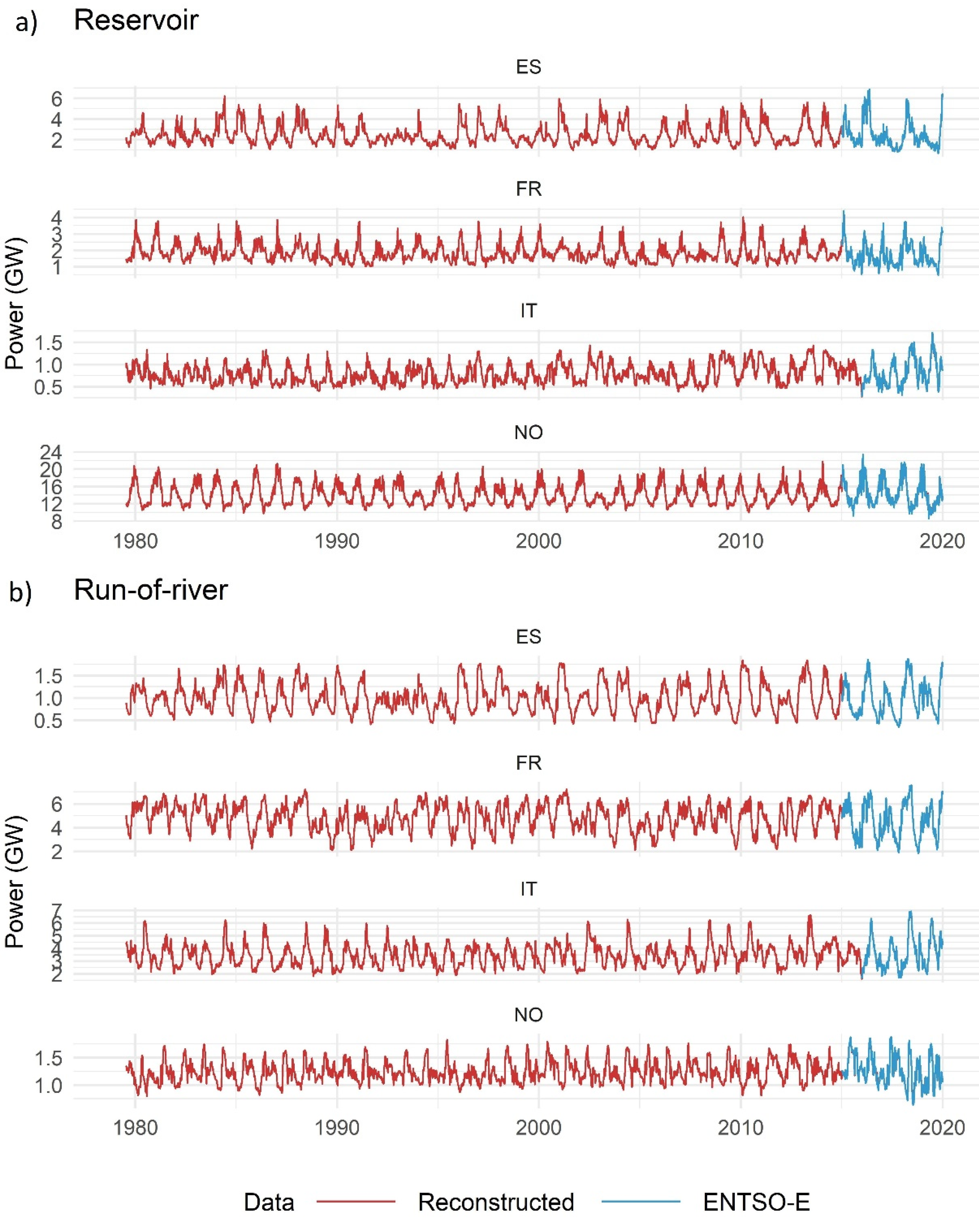
In order to produce a dataset of hydro power generation for the twelve countries of interest, country-specific models were trained again with the full observed ENTSO-E dataset for the period 2015–2019 using model 4 (multiple lags with temperature and precipitation). The model was then used with the full ERA5 time series data to extend the hydro power generation simulation to the historical period from 1979 to present—so called reconstructed data. While the focus of this paper is on the historical reconstruction over the past ca. 40 years, it is worth noting that the C3S Energy service is also developing similar datasets for two other cases: seasonal forecasts, up to six months ahead, and projections, up to 2100. The same model developed for the historical period is implemented in both of these cases.

Figure 4 illustrates time series of reconstructed hydro power generation using our selected model configuration compared against data from ENTSO-E for the four countries selected as representatives. The output data show similar patterns of seasonality as ENTSO-E data but somewhat smoother, especially in the case of reservoir-based generation, due to operation regulation according to electricity demand. However, we are confident that the main features of hydro power generation are well reproduced, in particular high- and low-generation events corresponding to low-frequency precipitation variability.

3.2. Validation with Independent Datasets

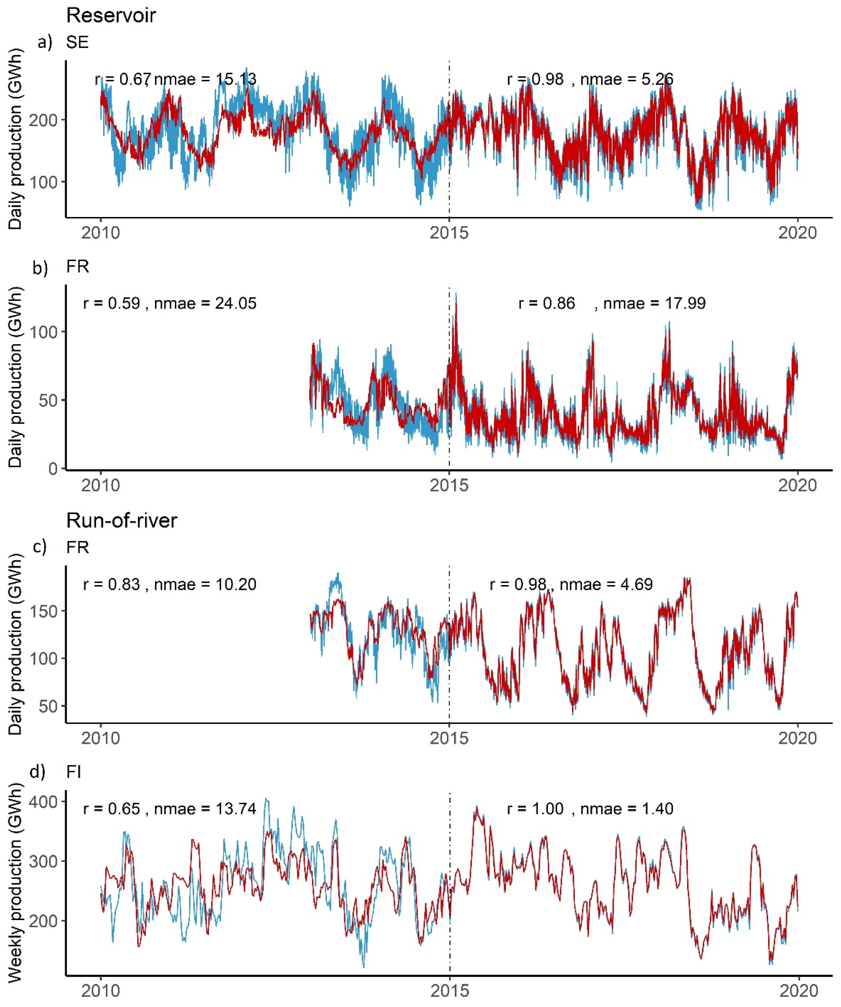
Although the two-step random forest model showed good performance, especially for Spain (Pearson’s correlation coefficient of 0.90 for reservoir-based and 0.98 for run-of-river generation from 5-fold cross-validation), this validation method usually gives optimistic results [16]. One possible explanation is that despite being randomly permuted, the validation dataset in each cross-validation is still an average of multiple random samples from the same dataset, and thus the prediction is not totally independent of the training set. As the model’s skill for extrapolation is important in producing historical (and eventually seasonal forecast, and projections) data, we conducted further tests with additional datasets from Réseau de Transport d’Électricité (RTE) for French hydro power generation in 2013–2014, and from Open Power System Data (OPSD) [17] data for Finland and Sweden in 2010–2014 (Figure 5).

Considering that the model only uses climate data and does not include any power plant information, these reconstructed time series show very encouraging results (see correlation coefficient indicated on each subplot). Specifically, the reconstruction for run-of-river generation captures the year-to-year variability in hydro power production remarkably well, with relatively high correlations (0.65 for FI, and 0.83 for FR) and relatively low NMAE values (13.7 for FI, and 10.2 for FR). While the performance is lower for reservoir-based hydro power generation, the difference is not large and, in any case, it is in line with that seen during the training period. The fact that our model is able to reconstruct the interannual variability of hydro power production reasonably well can be a very useful piece of information for system adequacy and extreme events assessments.

We can again see that the model performs better for run-of-river compared to reservoir-based generation here in the case of France. Reservoir time series have noticeably higher short-term variations. This is most likely due to reservoir operations managed by plant dispatchers to account for daily energy market dynamics. A model based on only climate data cannot capture these features, and hence the smoother predicted time series. However, the model is able to simulate the upward and downward trends of both hydro power generation types quite well, but it tends to underestimate the amplitude of the signal. As with every statistical model, it can only reproduce features that are embedded in the training period and, as such, it is limited in its ability to reproduce more extreme episodes. This is a common limitation of non-physical models which do not perform well in extreme cases.

3.3. The Sub-Country Level

One limitation of modelling hydro power is that averaging over a large domain such as country-size can smooth the characteristics of hydro power generation and neglect many physical aspects of the relevant water pathways. For instance, the river flow providing water for a given hydro power plant may come from a river basin in a neighbouring country and is therefore not considered. In addition, we consider country average temperature and precipitation, which could be a rough approximation, as a particular power plant will receive only water falling in the surrounding area, and not from the entire country. However, it is also the case that these considerations are very much country dependent, and different extensions and orography would need to be properly assessed in order to draw stronger conclusions.

To estimate the impact of geographical scales on our model, here, we test the model using the six Italian geographical bidding power zones. A geographical bidding zone is defined by ENTSO-E as a geographical area where market participants are able to exchange energy without transmission capacity allocation. Generation data at the bidding zone level is also available on the ENTSO-E Transparency Platform.

We chose Italy due to several factors. Firstly, only a few European countries have multiple bidding zones (for most of the countries, the bidding zone coincides with the country borders). Secondly, the Italian bidding zones provide a good mix of different installed hydro power capacities, orographic features, climatic characteristics, and zone sizes.

Italian bidding zones can be represented with an aggregation of nomenclature of territorial units for statistics [18] (NUTS) level 2 (or NUTS-2) regions. Since temperature and precipitation are provided at NUTS-2, these are first averaged (using a simple average; area-weights are assumed to be second-order effects) according to the bidding zone aggregation (see

Table 5. Average hydro power generation for the six Italian bidding zones, as well as for North and South Italy for the period 2015–2019.

Region	Bidding Zone	NUTS-2 Area Code	Daily Average Generation (MWh)
			Reservoir	Run of River
North	IT_North	ITC 1-4, ITH 1-5	1231.13	5486.23
South	IT_CNOR	ITI 1-3	71.40	464.23
	IT_CSUD	ITF 1 & 3, ITI 4	50.58	536.16
	IT_SUD	ITF 2, 4-6	122.02	233.23
	IT_SICI	ITG 1	8.08	21.40
	IT_SARD	ITG 2	33.48	12.65

). To assess the spatial scale effect, we aggregated the bidding zones into regions and country level and trained model accordingly to test its performance in these cases. The regional scale, i.e., North (IT_North in Table 5) and South Italy (the remaining 5 zones in Table 5), is based on geography and especially the different distribution of hydro power plants in Italy, with the North of Italy presenting the majority of the hydro power production. One of the corollaries is that the North and South of Italy are also considered as the main geographical subdivision of Italy as used in power trading (a discussion on the configuration of Italian bidding zones can be found at the following URL: https://docstore.entsoe.eu/Documents/cep/implementation/BZ/A4_BZR_ED_CSI_SQ.pdf). 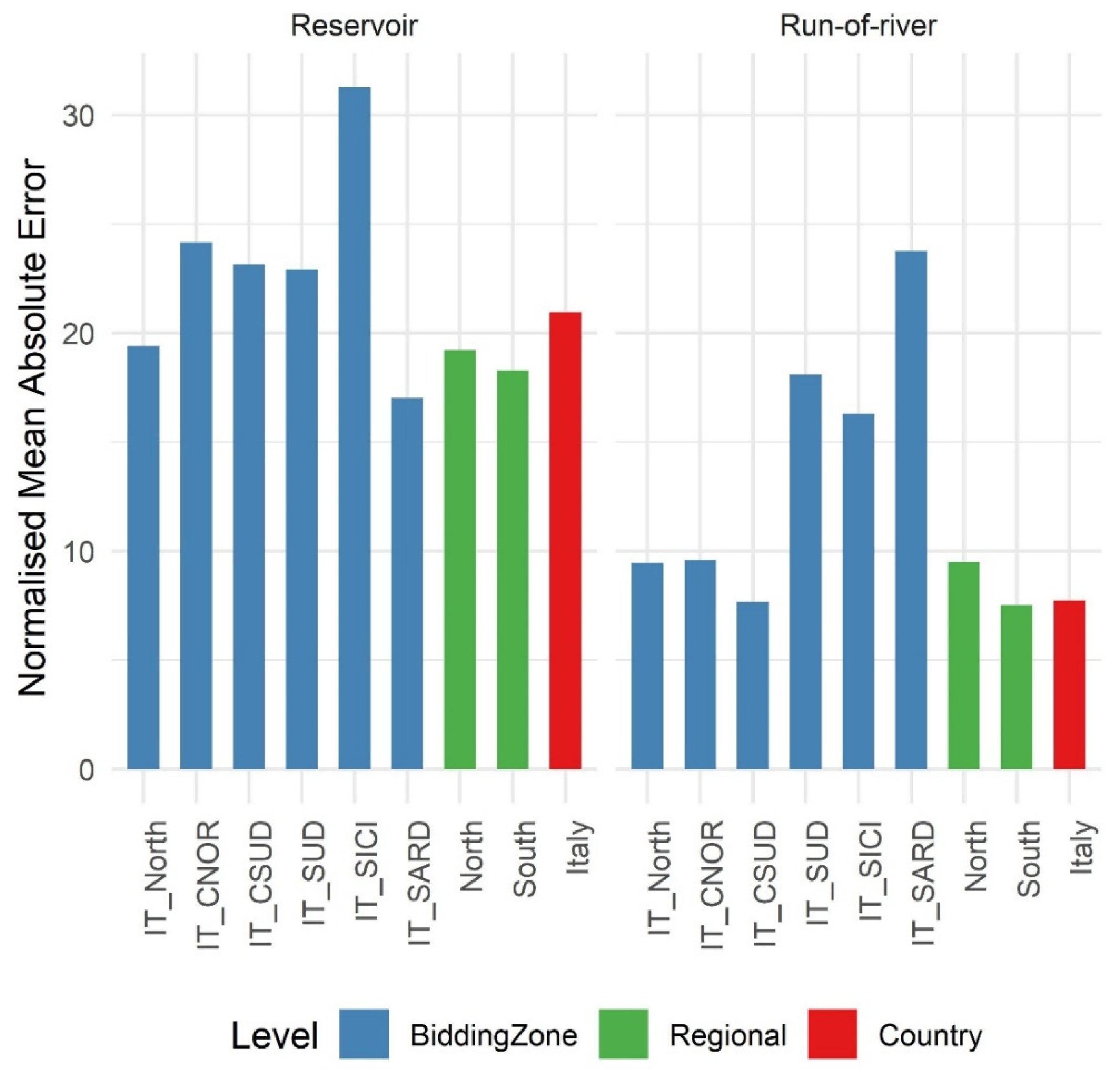Areas corresponding to bidding zones as well as to regions and their average generation are shown in Table 5.

Figure 6 shows the NMAE of the model implemented in these spatial scales. In general, the performance of the model for individual bidding zones is comparable to, or slightly worse than, that at the country level. Notable differences are for IT_SUD and IT_SICI, but especially for IT_SARD, for run-of-river generation. The main reason for this low performance is the very low installed capacities in these zones. Noting that the model performance at the country average level is very good (NMAE less than 10%) and therefore it is difficult to improve on it. It is also interesting to see that when bidding zones are aggregated in North and South Italy, the results are similar to the country average. These sub-country results demonstrate that a highly simplified hydro power model such as that used in our study has the potential to effectively simulate hydro power, therefore offering a credible complement to much more sophisticated physical models.

4. Summary and Discussion

We developed a new dataset of hydro power generation for reservoir-based and run-of-river generation using only two essential climate variables—temperature and precipitation—and a machine learning methodology, based on random forests, selected for its flexibility and accuracy. Model training was performed over the period 2015–2019. The reconstruction dataset was then developed for the historical period from 1979 to present, corresponding to the available period of the ERA5 climate reanalysis dataset (it will also be extended to seasonal forecast and climate projections). Snow melt has an important impact on river flow and, thus, on hydro power generation, but it is generally not available in seasonal climate forecast or climate projection outputs. Therefore, an approach was suggested using lagged values of temperature and precipitation to replace snow depth in the model. After testing two approaches with the optimal lag and multiple lags of temperature and precipitation, we found that multiple lags with a two-step approach to select the most important variables for each country and each hydro power type produced the best performance.

In general, the multiple lag approach yields better results than the optimal lag approach, particularly for run-of-river hydro power generation. In this case, we obtained a high average correlation of 0.95 and an average NMAE decrease of 10.23% compared to the optimal lag approach. Meanwhile, the model performance is expectedly lower in the case of reservoir hydro power generation, but still with a high correlation of 0.81 and an NMAE decrease of 5.98%. We also demonstrated that the inclusion of snow depth as an additional predictor does not, in general, lead to statistically better results. This model is inevitably subject to limitations.

An important limitation is that our methodology assumes constant installed capacities in all countries—both during training and reconstructed periods. This assumption does not take into account the periods in which plants are not available (e.g., for maintenance or due to temporary failures): in those periods, the actual generation data shows a drop that is not caused by meteorological factors. This information would be necessary to achieve better training of the machine learning models, thus for improving the simulation of the generation. In particular, in a cross-validation approach like that detailed in Section 3.1, this may explain some differences between the training and validation periods. Assuming constant installed capacity also ignores variations in other sources of energy. For instance, a newly installed wind farm might make the operator reduce electricity generated from a reservoir, but this effect is not captured by our model as it is not weather driven.

In addition, due to the complexity of hydro power plants, a statistical model cannot outcompete a physical model, especially when extrapolating to periods with climate characteristics outside of the observed range. Further, in our case, the training period is relatively short with five-year data for the period 2015–2019. In any case, one should keep in mind that the primary objective, developed in the context of C3S Energy is to provide a realistic method which can be readily implemented with publicly accessible datasets such as ENTSO-E. For example, [19] has produced a time series of reservoir-based generation in China using basin and power plant information. However, it is the first time a dataset of hydro power, which is also complemented by electricity demand, wind and solar power, has been produced at the European scale for both historical and future periods [20]. It is important to emphasize that the approach taken by C3S Energy is to model electricity demand and power generation over the ca. 40 year period, 1979 to present, assuming a fixed EU energy system based on available power data, which normally cover the last several years. From this dataset, actual energy generation and demand can be derived using simple arithmetic to rescale mean energy demand and generation based on actual installed capacity and annual energy consumption.

In terms of data quality, there is confidence in the model’s input data: [21] shows that precipitation and temperature variables from the ERA5 dataset can produce results equivalent to observational data in hydrological modelling from North-American catchments; [6] on the ENTSO-E dataset also highlights that it is the most ambitious global open source dataset for energy data.

Hydro power depends strongly on water availability, for which five years of training data could not accurately represent all the impacts of interannual climate variability. Bootstrap aggregation in random forest helps to avoid high-variance estimators from decision trees, i.e., a small change in input can alter the prediction results. Nonetheless, the fact that the model simulates hydro power production well (relatively low NMAEs and high correlations), especially over the extended periods available for France, Sweden and Finland, demonstrates that even a simple model, trained over a relatively short period, can capture essential (interannual) variability processes. It is also planned to update the models on a yearly basis, when an additional year of ENTSO-E data becomes available. This extension of the model training period is expected to improve the quality of the models over time.

Although random forest is known for its robustness against outliers, this feature reduces its ability to extrapolate to extreme events or to values outside of the training dataset, as shown in Section 3.2. In addition, when input variable deviation is large compared to their mean value, it is more difficult to differentiate between signal and noise, hence the lower performance in countries with smaller installed capacity such as run-of-river generation in Switzerland or both hydro power types in Slovakia.

Nevertheless, the model performance is encouraging, considering its simplicity and versatility. The presented results will be available in the C3S Climate Data Store later in 2020 and can serve as a benchmark for further studies on the impact of climate variability on hydro power.

References

1. EUROSTAT. Available online: https://appsso.eurostat.ec.europa.eu/nui/show.do?dataset=nrg_ind_peh&lang=en (accessed on 17 January 2020).
2. European Commission. Europe Leads the Global Clean Energy Transition: Commission Welcomes Ambitious Agreement on Further Renewable Energy Development in the EU; Statement/18/4155 14.6.2018; European Commission: Strasbourg, France, 2018. [Google Scholar]
3. Huertas-Hernando, D.; Farahmand, H.; Holttinen, H.; Kiviluoma, J.; Rinne, E.; Söder, L.; Milligan, M.; Ibanez, E.; Martínez, S.M.; Gomez-Lazaro, E.; et al. Hydro power flexibility for power systems with variable renewable energy sources: An IEA Task 25 collaboration. Wiley Interdiscip. Rev. Energy Environ. 2017, 6, e220. [Google Scholar] [CrossRef] [Green Version]
4. François, B.; Hingray, B.; Borga, M.; Creutin, J. Increasing Climate-Related-Energy penetration by integrating run-of- the river hydro power to wind / solar mix. Renew. Energy 2017, 87, 686–696. [Google Scholar] [CrossRef]
5. Copernicus Climate Change Service for the Energy Sector (C3S Energy). Available online: https://climate.copernicus.eu/operational-service-energy-sector (accessed on 17 January 2020).
6. Hirth, L.; Mühlenpfordt, J.; Bulkeley, M. The ENTSO-E Transparency Platform—A review of Europe’s most ambitious electricity data platform. Appl. Energy 2017, 225, 1054–1067. [Google Scholar] [CrossRef]
7. Copernicus Climate Change Service (C3S). ERA5: Fifth generation of ECMWF atmospheric reanalyses of the global climate. Copernicus Climate Change Service Climate Data Store (CDS). 2017. Available online: https://cds.climate.copernicus.eu/cdsapp#!/home (accessed on 9 January 2019).
8. Harrison, G.; Wallace, A.R. Sensitivity of hydro power performance to climate change. Int. J. Power Energy Syst. 2006, 26, 42. [Google Scholar]
9. Breiman, L.E.O. Random Forests. Mach. Learn. 2001, 45, 5–32. [Google Scholar] [CrossRef] [Green Version]
10. Ho, T.K. A Data Complexity Analysis of Comparative Advantages of Decision Forest Contructors. Pattern Anal. Appl. 2002, 5, 102–112. [Google Scholar] [CrossRef]
11. Hastie, T.; Tibshirani, R.; Friedman, J. The elements of statistical learning: Data mining, inference, and prediction; Springer: Berlin/Heidelberg, Germany, 2018. [Google Scholar]
12. Borges, C.L.; Pinto, R.J. Small hydro power plants energy availability modeling for generation reliability evaluation. IEEE Trans. Power Syst. 2008, 23, 1125–1135. [Google Scholar] [CrossRef]
13. De Felice, M.; Dubus, L.; Suckling, E.; Troccoli, A. The impact of the North Atlantic Oscillation on European hydro-power generation. Preprint 2018. [CrossRef] [Green Version]
14. Fisher, A.; Rudin, C.; Dominici, F. All Models are Wrong but Many are Useful: Variable Importance for Black-Box, Proprietary, or Misspecified Prediction Models, using Model Class Reliance. J. Mach. Learn. Res 2019, 20, 1–81. [Google Scholar]
15. Ng, J.Y.; Turner, S.W.; Galelli, S. Influence of El Niño Southern Oscillation on global hydropower production. Environ. Res. Lett. 2017, 12, 034010. [Google Scholar] [CrossRef]
16. Janitza, S.; Hornung, R. On the overestimation of random forest’s out-of-bag error. PLoS ONE 2018, 13. [Google Scholar] [CrossRef] [PubMed]
17. Open Power System Data (OPSD). Available online: https://open-power-system-data.org/data-sources#5_Hydro_power_data (accessed on 9 January 2019).
18. NUTS (nomenclature of territorial units for statistics). Available online: https://ec.europa.eu/eurostat/web/nuts/background (accessed on 17 January 2020).
19. Liu, H.; Andresen, G.B.; Brown, T.; Greiner, M. A high-resolution hydro power time-series model for energy systems analysis: Validated with Chinese hydro reservoirs. MethodsX 2019, 6, 1370–1378. [Google Scholar] [CrossRef] [PubMed]
20. Troccoli, A.; Goodess, C.; Jones, P.; Penny, L.; Dorling, S.; Harpham, C.; Dubus, L.; Parey, S.; Claudel, S.; Khong, D.H.; et al. Creating a proof-of-concept climate service to assess future renewable energy mixes in Europe: An overview of the C3S ECEM project. Adv. Sci. Res. 2018, 15, 191–205. [Google Scholar] [CrossRef]
21. Tarek, M.; Brissette, F.P.; Arsenault, R. Evaluation of the ERA5 reanalysis as a potential reference dataset for hydrological modeling over North-America. Hydrol. Earth Syst. Sci. Discuss. 2019, 1–35. [Google Scholar] [CrossRef]
Figure 1. Processes in the two-step random forest model with multiple lags.
Energies 13 01786 g001
Figure 2. The normalised mean absolute error and 95% confidence interval for reservoir (a) and run-of-river (b) types of the five models using inputs from k-fold cross-validation as follows: (1) baseline with daily temperature, precipitation, and snow depth in grey; (2) optimal lag of temperature and precipitation in blue; (3) same as second model + optimal lag of snow depth in orange; (4) multiple lags of temperature and precipitation in green (selected model); (5) same as (4) + multiple lags of snow depth in red. (TA = 2 metre temperature, TP = precipitation, and SD = snow depth.)
Energies 13 01786 g002
Figure 3. Scatter plots of hydro power generation for reservoir-based (a) and run-of-river (b) generation comparing ENTSO-E data on the x-axis and model reconstructed values on the y-axis for models (2) and (4): multiple lags of temperature and precipitation (green dots) and optimal lag (blue dots). In general, the multiple lags approach (Mult_TATP) performs better with less deviation and gives a larger improvement for run-of-river generation, while the optimal lag model (Opt_TATP) has a larger bias for extreme values.
Energies 13 01786 g003
Figure 4. Result of the model for the four countries with largest installed capacity, Spain (ES), France (FR), Italy (IT), and Norway (NO): 7 day rolling mean of reconstructed hydro power generation (GW) for reservoir-based (a) and run-of-river (b) generation for the period 1979–2019, namely a subset of the reconstructed dataset 1979–2019. Red line: reconstructed data; blue line: ENTSO-E data. As the model was trained for the period 2015–2019, the blue curve appears as overlapping with the red curve over this period.
Energies 13 01786 g004
Figure 5. Time series of observed (blue) and reconstructed (red) hydro power production of Swedish reservoir-based (a) in 2010–2014, French reservoir-based (b) and run-of-river (c) in 2013–2014 and Finnish run-of-river (d) in 2010–2014) generation. The dash-dotted vertical lines indicate 1 January 2015, marking the separation between the historical reconstruction (red curve left of the line) and the simulated data over the training period 2015–2019 (red curve right of the line). Note that observed data come from different sources: in the period 2010–2015, data are from non-ENTSO-E sources, e.g. Réseau de Transport d’Électricité (RTE) for France, and Open Power System Data (OPSD) for Finland and Sweden; while in the period 2015–2019, data are from ENTSO-E—the same source as the training period for the model, and hence the good agreement between red and blue curves over this period.
Energies 13 01786 g005
Figure 6. The normalised mean absolute error of the two-step random forest model applied to the six Italian bidding zones, as well as at the two regional aggregation areas (North and South), and at the country level for the period 2015–2019.
Energies 13 01786 g006