Crude Oil Prices Forecasting: An Approach of Using CEEMDAN-Based Multi-Layer Gated Recurrent Unit Networks

Abstract

Accurate prediction of crude oil prices is meaningful for reducing firm risks, stabilizing commodity prices and maintaining national financial security. Wrong crude oil price forecasts can bring huge losses to governments, enterprises, investors and even cause economic and social instability. Many classic econometrics and computational approaches show good performance for the ordinary time series prediction tasks, but not satisfactory in crude oil price predictions. They ignore the characteristics of non-linearity and non-stationarity of crude oil prices data, which hinder an accurate prediction and eventually lead to poor accuracy or the wrong result. Empirical mode decomposition (EMD) and ensemble EMD (EEMD) solve the problems of non-stationary time series forecasting, but they also generate new problems of mode mixing and reconstruction errors. We propose a hybrid method that is combination of the complete ensemble empirical mode decomposition with adaptive noise (CEEMDAN) and multi-layer gated recurrent unit (ML-GRU) neural network to solve the abovementioned issues. This not only deals with the issue of mode mixing effectively, but also makes the reconstruction error of data close to zero. Multi-layer GRU has an excellent ability of nonlinear data-fitting. The experimental results of real WTI crude oil dataset show that the proposed approach perform better in crude oil prices forecasts than some state-of-the-art models.

1. Introduction

Crude oil was once considered to be the blood flowing through the veins of the world economy and played an extremely critical role in the development of the world economy. According to a report by the U.S. Energy Information Administration (EIA), although renewable energy production and consumption both reached their highest share in 2018, fossil fuel still accounted for 80% of the United States’ energy consumption. In light of the International Energy Agency (IEA) data, the global consumption of oil reached 1.0075 million barrels per day in 2019. In meeting world energy needs, oil still plays the most important role. Asian emerging market countries have become the main contributors to the growth in crude oil demand. The rapid economic growth has prompted them to significantly increase demand for crude oil. For example, China’s oil consumption has soared from an average of 69,700 barrels per day in 2005 to 145,100 barrels per day in 2019. As a production factor, the increase in crude oil prices will lead to an increase in the non-oil companies’ production costs and a decrease in profits. Sadorsky [1] verified the impact of fluctuations in crude oil prices on companies of different firm size through evidence from the stock market. Rising oil prices may lead to inflation and hinder economic growth. Volatility in oil prices increases risk and uncertainty to financial markets [2]. Not only that, but the continued collapse or the sudden plunge in oil prices can also have a huge impact on the economic development and financial markets of oil-producing countries [3]. An obvious piece of evidence is the crisis signal coming from the credit default swap (CDS) market. The widening of the CDS spread means that weak crude oil prices have caused investors to worry about the fiscal sustainability of some oil producing countries [4]. The study of Haushalter et al. [5] concluded that there is a negative correlation between the price of crude oil and the debt ratio of oil producers.

Based on the above discussion, it is obviously of great significance to find a method that can accurately predict the price of crude oil. This means that policy makers will have more time to introduce countermeasures to achieve the goal of avoiding or reducing risks. However, the trend of oil prices is affected by not only the factors of market supply and demand, but also the other non-market factors, such as geopolitical, alternative forms of energy, recession, war, natural disasters, and technological development. Various uncertainties affect the crude oil market. The fluctuations in these factors cause the nonlinear, volatile, and chaotic tendency of crude oil prices. Therefore, achieving sufficiently reliable and accurate forecasting of crude oil prices has become one of the most challenging issues.

In the past decades, various techniques have been tried to forecast the trend of crude oil prices. The classic statistical or econometric models such as autoregressive integrated moving average (ARIMA) model and the autoregressive conditional heteroskedasticity (ARCH)/generalized ARCH (GARCH) family model are widely used in the time series prediction tasks [6,7,8,9,10,11,12]. Zhao and Wang [9] used the ARIMA model to model and predict crude oil prices based on the international crude oil prices data from the 1970s to 2006. Mohammadi and Lixian [13] applied the ARIMA-GARCH model to forecast the conditional mean and volatility of weekly crude oil spot prices in eleven international markets. Aamir and Shabri [14] used the Box-Jenkins ARIMA, GARCH and ARIMA-Kalman models to model and forecast the monthly crude oil prices in Pakistan. The premise of applying these classic models represented by ARMA /ARIMA is that there is an autocorrelation in the crude oil prices series. So, the historical data is used to infer the future prices of crude oil. These methods are suitable for capturing the linear relationships in time series analysis but not for the nonlinear time series [15]. In addition to the classical methods mentioned above, the survey forecasting method is another alternative method for crude oil price forecasting [16]. Kunze et al. [17] empirically studied the performance of survey-based predictions of crude oil prices. The evaluation shows that the prediction accuracy of the survey-based forecasts is not as good as that of the naive method in the short-term crude oil prediction, but with the rise of the prediction horizon, the accuracy of the former will exceed that of the naive method. This study demonstrates that survey predictions are not suitable for the short-term prediction of crude oil prices.

Owning to the drawbacks of the classic approaches and the special features of crude oil price data, artificial intelligence (AI), such as machine learning, deep learning or hybrid methods provide more excellent nonlinear data predictive performance. In term of forecasting crude oil prices, the approaches of AI are being widely used as alternative to the classic technologies. Li et al. [18] proposed an approach that incorporates ensemble empirical mode decomposition (EEMD), sparse Bayesian learning (SBL), for forecasting crude oil prices. Xie et al. [19] used support vector machines to forecast crude oil prices and compared the performance with ARIMA and BPNN’s. Experiments show that SVM has better performance than the other two methods. Fan et al. [20] propose an independent component analysis based SVR scheme, for crude oil prices predictions. This approach starts from an independent component analysis to decompose crude oil prices series into independent components, which are respectively forecasted by support vector regression (SVR).

Crude oil prices trends have significant nonlinear and non-stationary characteristics. Regardless of the traditional statistics or machine learning methods, it is difficult to obtain satisfactory results by directly predicting the original crude oil prices series. Therefore, scholars usually adopt the method that, first, the original crude oil prices series is decomposed into multiple same time scales or relatively simple sub-sequences by a signal decomposition algorithm. Next, create multiple subtasks. Each sub-task completes the prediction of a sub-sequence individually. Finally, the results of all subtasks are linearly calculated and the forecasting is obtained. Common signal decomposition methods, such as the wavelet transform, EMD, and EEMD, have been widely used to process the non-stationary time series. Yu et al. [21] proposed an EMD-based neural network crude oil price forecasting. He et al. [22] come up with a wavelet-based ensemble model to improve the predictive accuracy of oil prices. This approach introduced the wavelet to generate dynamic basic data within a finer time-scale domain. Hamid and Shabri [23] proposed a wavelet multiple linear regression method in daily forecasts of crude oil price. Wu et al. [24] propose a model based on EEMD and long short-term memory (LSTM) for crude oil price forecasting. Zhou et al. [25] introduced a hybrid approach of complete ensemble empirical mode decomposition with adaptive noise (CEEMDAN) and XGBOOST-based approach to forecast crude oil prices.

Both wavelet analysis and EMD are becoming the common tools for analyzing non-stationary time series but have their own limitations. The wavelet method can’t achieve an adaptive decomposition in the light of time scales. It has been proven above that EMD perform well in extracting signals from the non-stationary data. Mode mixing is the main limitations of EMD. It is a consequence of signal intermittency which could result in the physical meaning of individual intrinsic mode function (IMF) unclear [26]. To overcome this limitation of EMD, an ensemble EMD named EEMD, was subsequently introduced by Wu and Huang [27]. EEMD adds white noise to the original signal. After a sufficient number of EMD tests, the only lasting component of signal is then identified as the substantial answer. EEMD eliminates the effects of mode mixing of EMD, but still retains some noise in the IMFs, which affect the accuracy of signal reconstruction [28].

In summary, much effort has been made to improve the accuracy of forecasting crude oil prices, but a more effective approach should be developed. The goal of this study is to propose a new novel approach of CEEMDAN-based multi-layer gated recurrent unit networks (CEEMDAN-ML-GRU). CEEMDAN is a variant of EEMD. In the applying of CEEMDAN, the multiple groups of adaptive white noise is added to the original data at each stage of the decomposition and a unique residue is computed to obtain each mode. CEEMDAN is complete, with a numerically negligible error of signal reconstruction. Due to the excellent characteristics of CEEMDAN, in recent years, some researchers have tried to apply it to no-stationary time series analysis [29,30]. The gated recurrent unit (GRU), like LSTM, is a recurrent neural network with a gating mechanism, but it has fewer parameters than LSTM, as it lacks an output gate. GRU’s performance on certain tasks was found to be similar or even better to that of LSTM. A GRU network with a multi-layer stack structure has more powerful performance than a single-layer structure. The following experiments show that our proposed hybrid model goes on better than some other state-of-the-art’s in oil price forecast.

The content of this paper is organized as follows: Section 2 review the background works related to our method. Section 3 introduce the proposed method in detail, Section 4 applies the proposed approach to forecast crude oil prices of West Texas Intermediate (WTI), then compares it with other standard models and some state-of-the-art hybrid models. Finally, Section 5 concludes the study and summarizes several main interesting issues for future research.

2. Related Work

This section will briefly review the existing works that closely relate to our proposed approach.

2.1. Artificial Neural Networks (ANN)

ANN is made up of many "neurons", whose output can be the input of another neuron. One kind of classic ANN, the multilayer perceptron (MLP) is illustrated in Figure 1. In the graph illustrated in this figure, the variable X represents the input, and the circles represent the "neurons" of the network. This ANN has three layers which relative positions, arranged from left to right, are in sequence: input layer, output layer, and hidden layer. In Figure 1, the circles represent the nodes of the network.

There are m input neurons (nodes), n hidden neurons (nodes) and one output neuron (node) in this network that each layer of neurons receives inputs from the previous layers. This type of network is also called a multi-layer feedforward network, where the output of a node in one layer is the input of the next layer. The nodes in the hidden layer receive the output of the previous layer and perform weighted linear combination of the inputs. The result is then modified by an activation function before being output. We introduce several concepts that are closely related to neural networks:

(1)

Activate Function, it can normalize the output to a given range to ensure that the model is convergent. Each neuron accepts input and passes it through an activation function. The commonly used activation functions include Sigmoid, Tanh and ReLu.

(2)

Backpropagation, it is an algorithm commonly used to train the neural networks. After the inputs are loaded into the network, they pass forward through the neural network. Given an initial weight, the network provides an output for each neuron. When there is an error between the classification or regression results and the observations, the back-propagation mechanism comes into play. It helps to adjust the weights of the neurons, bringing the results closer and closer to the known true results.

(3)

Optimization algorithm, they are commonly used mathematical techniques in neural network optimization, and use the backpropagation to calculate the gradients. An example is gradient descent, the most common optimization method. In each training cycle, the best strategy for parameter (weight) adjustment is determined by observing the derivative of the error function with respect to each parameter. It enables the parameters to be updated in the negative gradient direction of the error function during each training to achieve the purpose of minimizing the error. In deep learning, the commonly used optimizers include stochastic gradient descent (SGD), adaptive gradient algorithm (Adagrad), adaptive moment estimation (Adam), etc.

2.2. Backpropagation

In ANN, especially in deep learning, backpropagation is an algorithm widely used to train feed-forward neural networks for supervised learning. The backpropagation algorithm is to compute the gradient of the loss function with respect to each parameter by the chain rules, and iterate backward from the last layer to avoid repeating calculation of the intermediate term of the chain. All of deep learning models mentioned later, such as recurrent neural network (RNN), LSTM and GRU use the backpropagation for training the network. The MLP is also shown in Figure 1.

Given a training set of m examples. The backpropagation algorithm is as follows:

(1) Perform a forward propagation, and so on up to the output layer.

$$Z_i^{l+1}={{\displaystyle \sum }}_{j=1}^m{W}_{ij}^{\left(l\right)}{x}_j+b_i^{\left(l\right)}$$

(1)

$$S_i^{\left(l+1\right)}=\sigma \left(Z_i^{l+1}\right)=\sigma \left({{\displaystyle \sum }}_{j=1}^m{W}_{ij}^{\left(l\right)}{x}_j+b_i^{\left(l\right)}\right)$$

(2)

$$F_{W,b}^{\left(l+1\right)}\left(X\right)=\sigma \left({{\displaystyle \sum }}_{i=1}^n{S}_i^{\left(l+1\right)}+b_i\right).$$

(3)

The (W,b) is the parameter where $W_{ij}^{\left(l\right)}$ denote the weight associated with the connection between unit i in layer l, and unit j in layer l + 1. $b_i^{\left(l\right)}$ is the bias associated with unit i in layer l. $\sigma$ denotes the sigmoid function, which can transform the data into a value in the range of 0–1, thereby serving as a gate signal. $S_i^{\left(l\right)}$ denote the activation of unit i in layer l. The computation steps of the neural network Figure 1 represent is given by:

$$\begin{gathered} S_1^{\left(2\right)}=\sigma \left(W_{11}^{\left(1\right)}{x}_1+W_{12}^{\left(1\right)}{x}_2+W_{13}^{\left(1\right)}{x}_3+b_1^{\left(1\right)}\right) \\ {S}_2^{\left(2\right)}=\sigma \left(W_{21}^{\left(1\right)}{x}_1+W_{22}^{\left(1\right)}{x}_2+W_{23}^{\left(1\right)}{x}_3+b_2^{\left(1\right)}\right) \\ {S}_3^{\left(2\right)}=\sigma \left(W_{31}^{\left(1\right)}{x}_1+W_{32}^{\left(1\right)}{x}_2+W_{33}^{\left(1\right)}{x}_3+b_3^{\left(1\right)}\right) \\ {F}_{W,b}\left(X\right)=S_1^{\left(3\right)}=\sigma \left(W_{11}^{\left(2\right)}{S}_1^{\left(2\right)}+W_{12}^{\left(2\right)}{S}_2^{\left(2\right)}+W_{13}^{\left(2\right)}{S}_3^{\left(2\right)}+b_1^{\left(2\right)}\right) \end{gathered}$$

(2) Define the overall cost function to be:

$$C_{W,b}=\frac{1}{m}{{\displaystyle \sum }}_{i=1}^m\left(\frac{1}{2}{\Vert F_{W,b}\left(X\right)-Y\Vert }^2\right)$$

(4)

This cost function is used to compute error between the actual output and the expected output.

(3) Compute the partial derivatives with respect to (W,b):

$${\delta }_j^L=\frac{\partial C_{W,b}}{\partial S_i^{\left(l\right)}}{\sigma }^{\prime }\left({{\displaystyle \sum }}_{i=1}^n{S}_i^{\left(l+1\right)}+b_i\right)$$

(5)

The derivative tells us the direction of movement of the weight values and how to get a lower cost in the next iteration.

2.3. Gradient Descent (GD)

In neural networks or deep learning, GD is one of the most common optimization algorithms used to minimize the loss function by iteratively moving in the steepest direction. The process of updating the parameters (W,b) in one iteration of GD is as shown below:

(1)

Initialize the $\mathsf{\Delta }{W}^{\left(l\right)}$ and $\mathsf{\Delta }{b}^{\left(l\right)}$.

(2)

Use backpropagation to compute ∇W^(l) $C_{W,b}$ and ∇b^(l) $C_{W,b}$.

(3)

Set: $\mathsf{\Delta }{W}^{\left(l\right)}:=\mathsf{\Delta }{W}^{\left(l\right)}+{\nabla }_{W^{\left(l\right)}}{C}_{\left(W,b;x,y\right)},\mathsf{\Delta }{b}^{\left(l\right)}:=\mathsf{\Delta }{b}^{\left(l\right)}+{\nabla }_{b^{\left(l\right)}}{C}_{\left(W,b;x,y\right)}$

(4)

Update the parameters:

$$W_{ij}^{\left(l\right)}=W_{ij}^{\left(l\right)}-\alpha \frac{\partial }{\partial W_{ij}^{\left(l\right)}}{C}_{\left(W,b\right)}$$

(6)

$$b_i^{\left(l\right)}=b_i^{\left(l\right)}-\alpha \frac{\partial }{\partial b_i^{\left(l\right)}}{C}_{\left(W,b\right)}$$

(7)

where α is the learning rate, which specifies how aggressively the gradient descent should jump between successive iteration.

3. Methodology

This section will not only detail the method proposed in this paper, but also introduce some models that are closely related to the proposed method. They include signal processing algorithm such as EMD, EEMD and CEEMD, recurrent neural networks such as RNN, GRU and ML-GRU.

3.1. EMD, EEMD and CEEMDAN

Through EMD, the nonlinear and non-stationary signal can be adaptively decomposed into the limited IMFs based on local characteristic of time scales. The essence of this method is to eliminates the interference of noise and identify the intrinsic oscillatory modes in the data empirically. To obtain the valuable instantaneous frequencies, the IMFs must satisfy two conditions:

(1)

The numbers of extremes and zero crossings of the sequence must be equal or differ by no more than one.

(2)

At any location, the mean of the envelope determined by the local extrema is zero [26].

The EMD is developed as follows:

Connect all the local maxima (minima) with a cubic spline as the upper (lower) envelope.

Get the first IMF by calculating the difference between the original data and local mean envelope:

$$M\left(t\right)=\frac{1}{2}\left[U\left(t\right)-L\left(t\right)\right]$$

(8)

$$\mathrm{IMF}\left(t\right)=X\left(t\right)-M\left(t\right)$$

(9)

where $U\left(t\right)$ and $L\left(t\right)$ are the upper envelope and the lower envelope respectively. If the difference original data X(t) to the mean envelope (M(t) meets the IMF constraints, this difference is the new IMF.

The result of subtracting all the previous IMFs from original data is the current residue. Using the residue as the new input and repeating the above procedure, the next IMF can be obtained:

$$R_K\left(t\right)=X\left(t\right)-{{\displaystyle \sum }}_{i=1}^K{\mathrm{IMF}}_i$$

(10)

$${\mathrm{IMF}}_{K+1}\left(t\right)=R_K\left(t\right)-{\mathrm{IMF}}_{K+1}$$

(11)

where $R_K\left(t\right)$ is the residue series after K-th decomposition. A complete decomposition process stops when the residue, $R_K\left(t\right)$, has been a monotonic function.

There are some drawbacks in EMD, mainly as follows: (a) In IMFs mode mixing exists. It means that the IMFs composed of oscillations of different time-scales and no longer have physical meaning. (b) The effects of end affect the results of decomposition. To overcome the drawbacks, Huang et al. [27] introduced a novel EEMD approach that utilizes the advantages of white noise to eliminate the effects of mode mixing. After EEMD, the reconstructed data includes residual noise and disparate parameters of noise can produce disparate number of modes [28].

CEEMD, proposed by Torres et al. [28]. The final decomposition result is obtained by taking the average by adaptively adding white noise to the time series with the same magnitude and opposite direction. After engaging in EMD processing, the output of CEEMDAN obeys a Gaussian distribution. Compared with EEMD and CEEMD, this method effectively eliminates the problem of mode mixing, and no matter how many times the decomposition, the reconstruction error of the signal is almost zero, the completeness is better, and at the same time solves the problem of low decomposition efficiency, greatly reducing the calculation cost. CEEMDAN’s spectra shows a more accurate decomposition of the frequency than the EEMD’s. The same time series, the number of iterations of CEEMDAN shifting is usually equivalent to half of the EEMD’s.

The implementation of the algorithm is summarized as follows:

Generate a white noise plus series $\left(x_i\left(t\right)=x\left(t\right)+w_i\left(t\right)\right)$. Here, $w_i\left(t\right)$ denote the white noise of finite variance, while $x\left(t\right)$ represent the original data. Then decompose $x_i\left(t\right)$ to obtain the IMFs:

$$\overline{im{f}_i}=\frac{1}{n}{\displaystyle {\displaystyle \sum }_{j=1}^n}im{f}_i^j\left(t\right)$$

(12)

where $w_i^j\left(t\right)$ is the white noise added at the j-th time with the mean equal to zero and variance equal to one. The $\overline{im{f}_i}$ is the i-th mode component obtained after the signal is decomposed by CEEMDAN.

Calculate the first residue:

$$r_1\left(t\right)=x\left(t\right)-\overline{im{f}_1}$$

(13)

Decompose the residue to get the second IMF and calculate the second residue:

$$\overline{im{f}_2}=\frac{1}{n}{{\displaystyle \sum }}_{j=1}^n{E}_1\left\{r_1\left(t\right)+{\epsilon }_1{E}_1\left[w_2^j\left(t\right)\right]\right\}$$

(14)

$$r_2\left(t\right)=r_1\left(t\right)-\overline{im{f}_2}$$

(15)

Decompose the (k − 1)th residue of $r_{k-1}\left(t\right)$ and extract the $\overline{im{f}_k\left(t\right)}$. The process can be demonstrated in the following equation (k = 2, 3, … K):

$$\overline{im{f}_k\left(t\right)}=\frac{1}{n}{{\displaystyle \sum }}_{j=1}^n{E}_1\left(r_{k-1}\left(t\right)+w_{k-1}^j{E}_{k-1}\left({\epsilon }^j\left(t\right)\right)\right)$$

(16)

Calculate the k-th residue:

$$r_k\left(t\right)=x\left(t\right)-{{\displaystyle \sum }}_{i=1}^{k}im{f}_i$$

(17)

where k indicates the number of IMFs. The attributes of the original time series are denoted by all the IMFs exacted from different time-scales. The only residue demonstrates the trend, which is smoother than that of the original time series.

3.2. GRU and Multi-LayerML-GRU

3.2.1. RNN and GRU

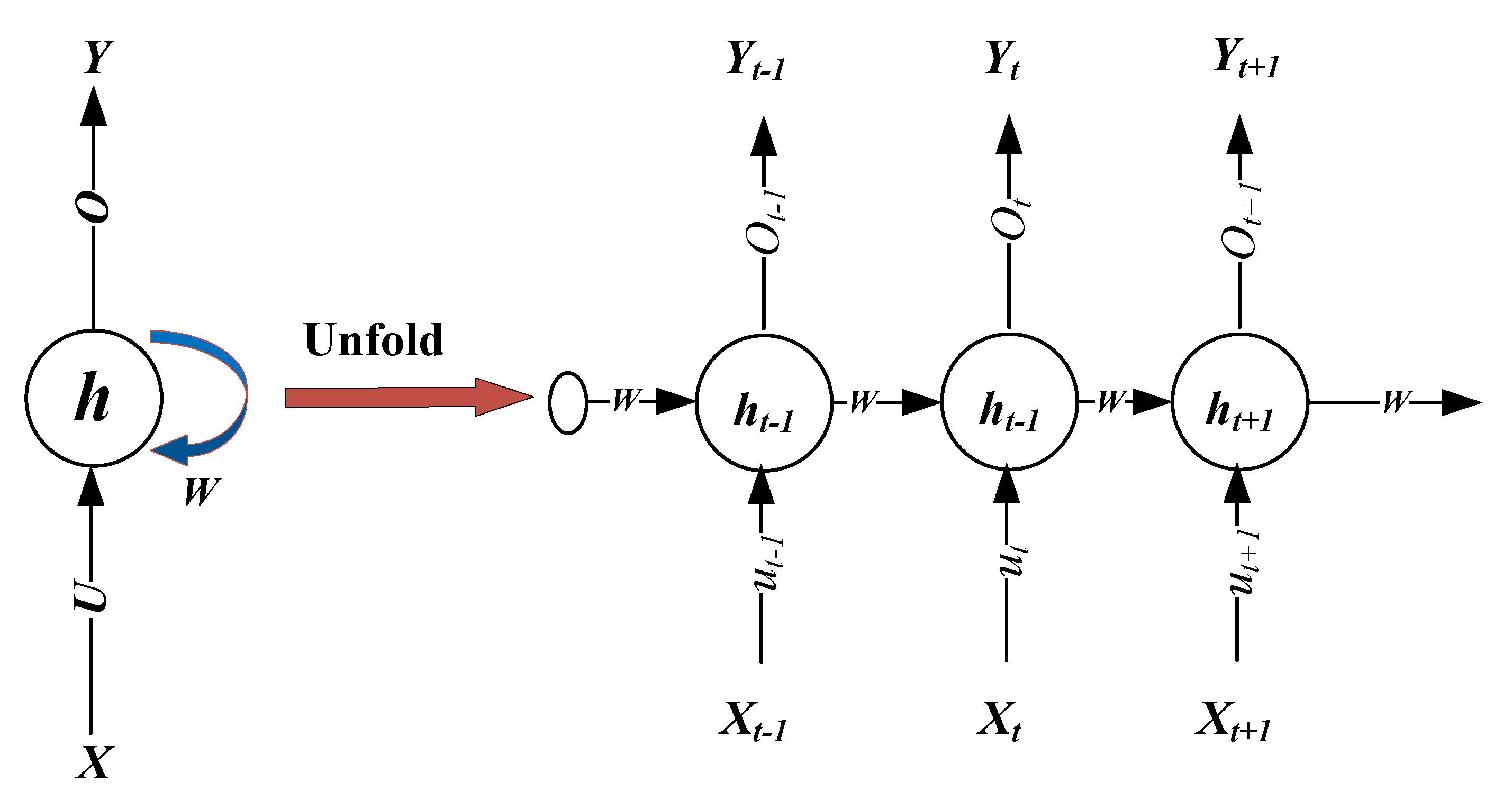
Among deep learning methods, RNN is a powerful method for processing time series data. It is widely used in many fields such as finance [31,32], industry and engineering [33], machine translation [34], speech recognition [35], economic prediction [36], and so on. As shown in Figure 2, RNN has certain information persistence capabilities, which enable information to be passed from one time-step to the next. However, the classic RNN does not have the ability to store and memorize data for a long time, so that it cannot capture long-term historical information. In addition, in the reverse process of model training, once the sequence is too long, the RNN will cause the problem of gradient explosion or gradient disappearance. To overcome these drawbacks, Hochreiter and Schmidhuber [37] proposed the LSTM neural network which is capable of learning long-term dependencies of time series, as well as forgetting the worthless information based on the current input. LSTM has since replaced RNN as the most widely used recurrent neural network. LSTM has four gated unit that capable adaptively regulate the information flow inside the unit. An LSTM neural network usually requires many gated units, which need train a large number of parameters and occupy more computing resources. In order to reduce the training parameters and simply the neural network, Cho et al. [38] proposed a neural network named GRU which only have two gated units in the hidden unit.

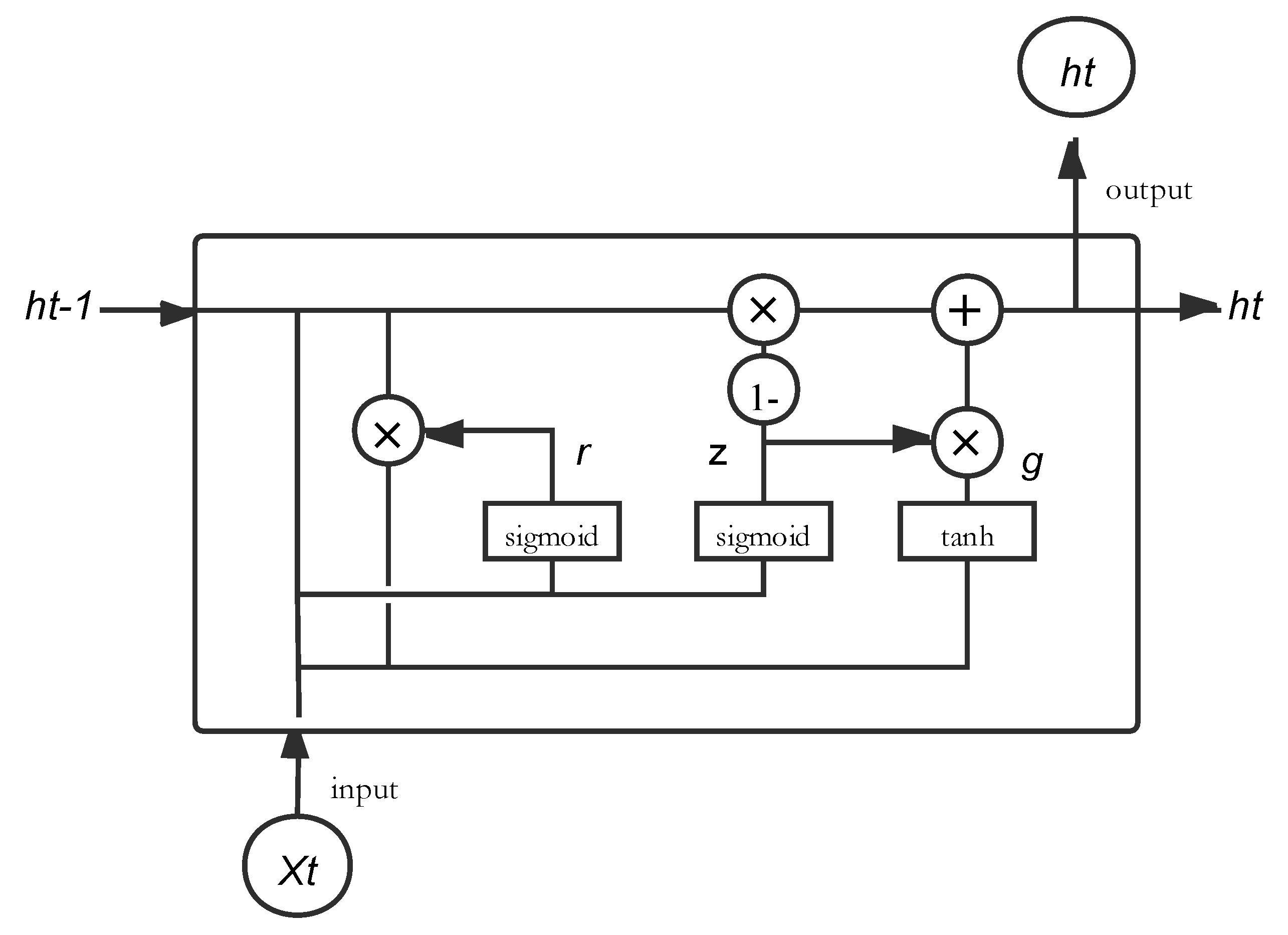
As one of the variants of RNN, the input and output structure of GRU neural network is the same as that of RNN and LSTM, as shown in the Figure 3 The neurons of GRU receive the hidden state (h_t−1) of the neuron of the previous neuron, and the current input x_t. After passing through the gating unit, the neural network gets the output y_t and passes the hidden state h_t to the next neuron.

The GRU architecture, like LSTM, learns the long-term dependence of time series based on a gate mechanism that includes reset gate and update gate. The former is used to control how much information in the previous state will be ignored. The latter is used to control how much information from the historical state is brought into the current state. GRU neural networks, like other neural networks, consist of a large number of basic neurons. They are interconnected in a complex network. A single neuron cell is shown in Figure 2. The specific process is designed as follows:

$$z_t=\sigma \left(w_{xz}{x}_t+w_{hz}{h}_{t-1}\right)$$

(18)

$$r_t=\sigma \left(w_{xr}{x}_t+w_{hr}{h}_{t-1}\right)$$

(19)

The internal structure of the GRU cell is shown in Figure 3.

The update gate is used to control the extent to which the state information from the previous moment is retained to the current state. The more the value of the update gate approaches 0, the more the state information from the previous moment is brought into the current state. The update gate signal is the closer to 0, the more data it remembers. The closer to 1, the less it is forgotten.

Begin with getting the gating signal, GRU gets the reset data through the gate; then combine it with the input $x_t$, and use a tanh activation function to shrink the data to the range from −1 to 1. The formula is shown in the following:

$$g_t=\tan h\left(w_{xg}{x}_t+w_{hg}\left(r_t\times h_{t-1}\right)\right)$$

(20)

The last step of GRU, we can call it "update memory" phase. Combined with the previous discussion, this step forgets some of the dimensional information passed in and add some new information inputted by the current neuron to the state variable $h_t$:

$$h_t=\left(1-z_t\right)\times h_{t-1}+z_t\times g_t$$

(21)

3.2.2. Multi-Layer GRU Architecture

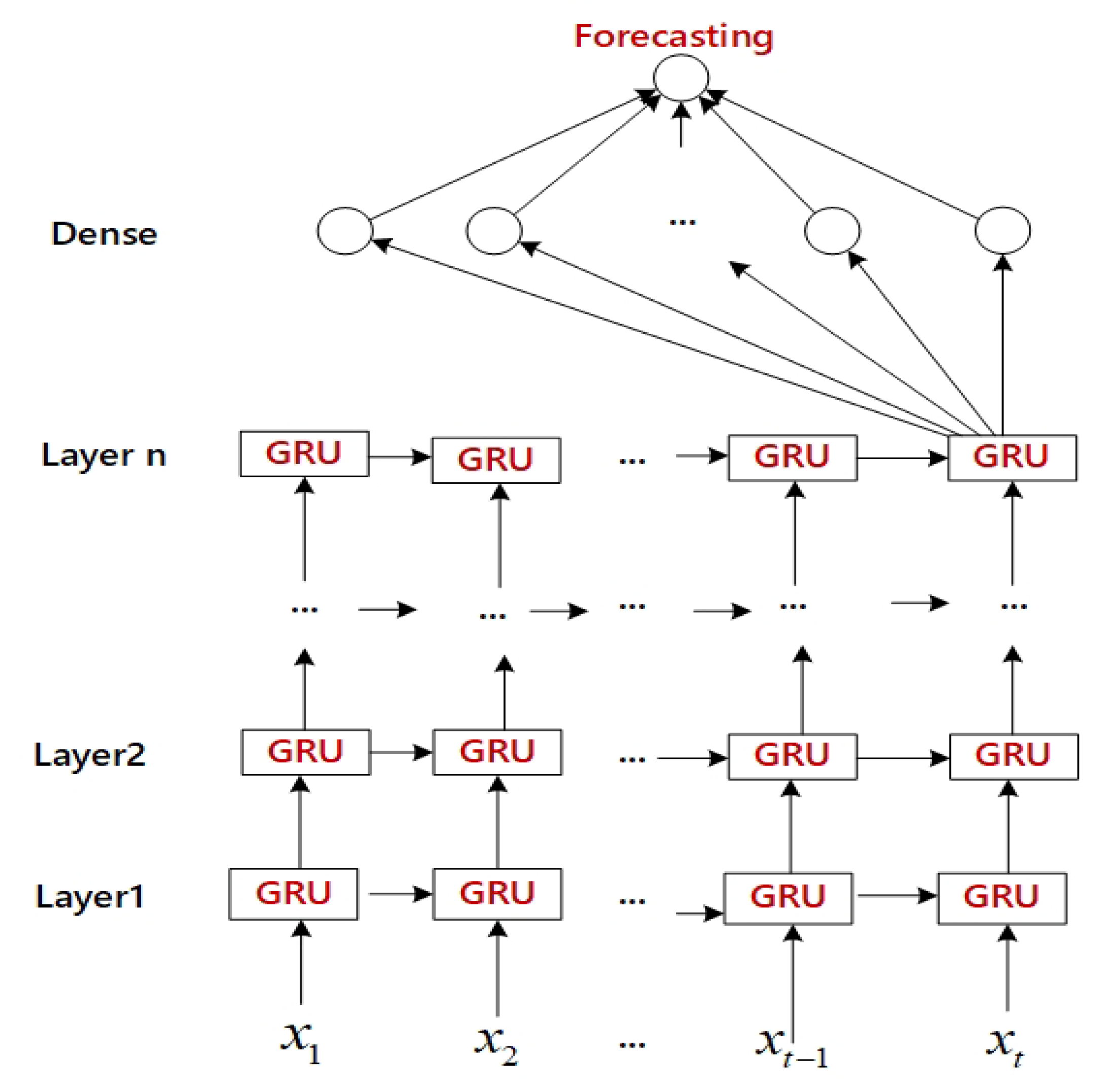
If the problem is too complicated, a recurrent neural network with a single layer structure is not enough to abstract the problem, and a multi-layer neural network is a better alternative. The multi-layer neural network has more hidden layers and more powerful computing capabilities which is the key to solving complex problems. The proposed model is one kind of forward multi-layer neural networks, which demand the input layer are required to have the same number of input dimensions as the input vector. The architecture and workflow of the ML-GRU are shown in Figure 4. The output dimensions of the last layer demand only be equal to the number of labels for classification or a single value of prediction for regression. With each training, the parameters are continuously updated. This process continues until the output of the network is closer to the desired output.

The multi-layer architecture determines that data flows through more neurons and more parameters need to be trained, as well as more powerful than the single layer network. If the recurrent neural network is too deep beyond what is necessary, the computational cost will be expensive. Also, the phenomenon of overfitting may occur.

3.3. CEEMDAN-Based Multi-Layer Gated Recurrent Unit Networks (CEEMDAN-ML-GRU)

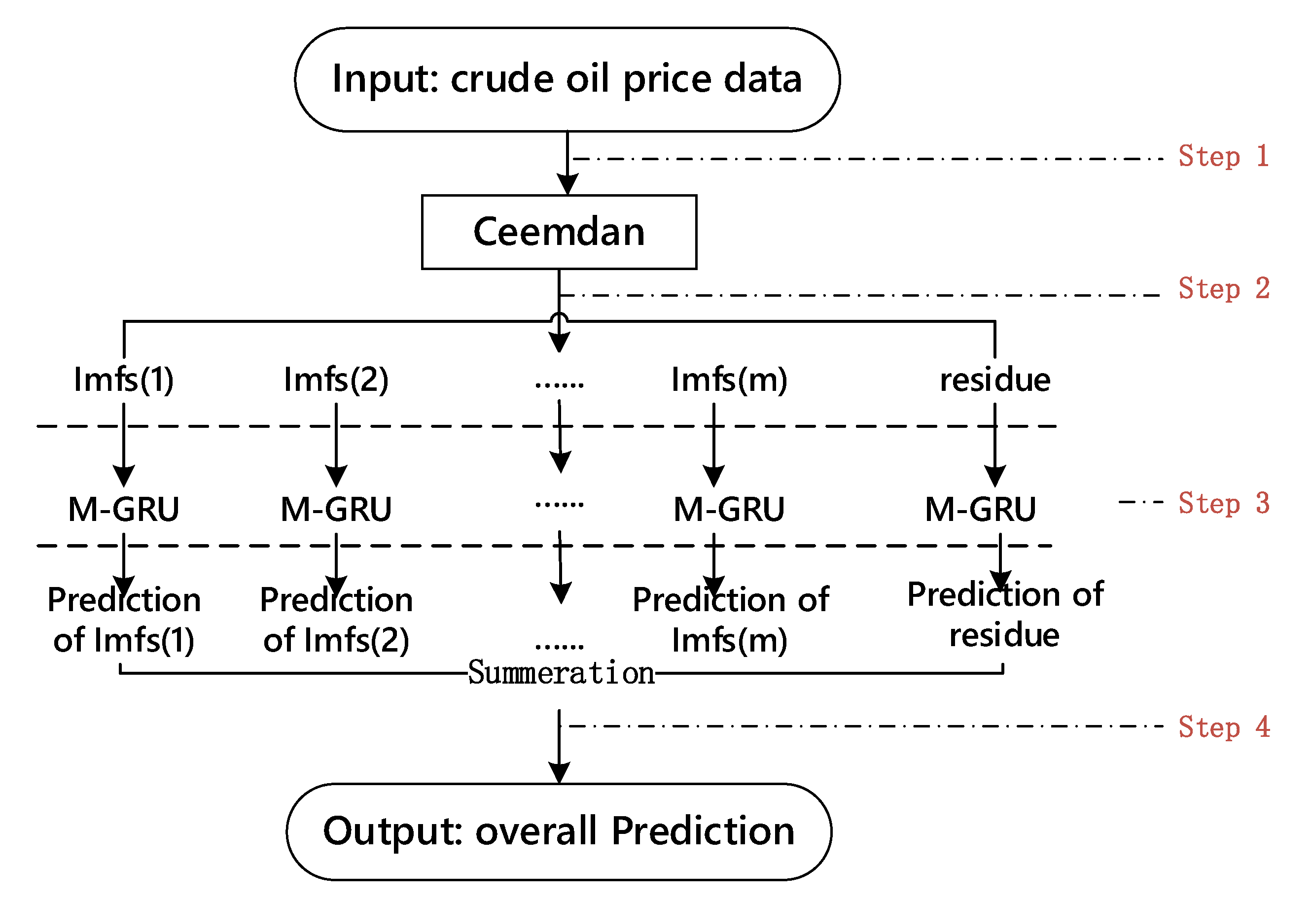
In this study, we introduce a novel approach combining CEEMDAN and multi-layer GRU neural networks. We call this model CEEMDAN-ML-GRU for crude oil price forecasts. Figure 5 shows the architecture and workflow of the hybrid model. It aimed at improving the exiting crude oil price forecast techniques, which are less efficient or have poor accuracy in dealing with nonlinear and nonstationary regression tasks.

Firstly, CEEMD technology is used to add positive and negative paired white noise to the original exchange rate sequence, which overcomes the problem of large EEMD reconstruction errors and poor completeness of decomposition, and effectively improves the decomposition efficiency. Then the original exchange rate sequence is decomposed into IMFs based on different characteristics. Finally, the multi-layer LSTM based forecasting model is input for each component, and each of the IMF prediction results is superimposed to obtain the desired overall prediction.

As mentioned in the introduction, signal decomposition techniques such as wavelet transform, EMD and EEMD have been used for the analysis of time series of predicting energy prices. Machine learning, especially neural networks and deep learning methods, have also been applied to crude oil price forecasting to improve the learning process and prediction accuracy of crude oil price data. Signal decomposition technology is good at processing non-stationary data, and deep learning shows excellent performance when analyzing time series with nonlinear and long-term dependency characteristics. Some scholars have proved that integrating signal decomposition and deep learning methods for crude oil prices forecasting gained better results than only using a single method. In Section 1, we have mentioned that Wu et al. [24] proposed a novel model based on EEMD and long LSTM for crude oil price forecast. We will compare them experimentally with the proposed method in the next section. This kind of hybrid model is able to synthesize the strengths of each hybrid method, and significantly avoids the negative impact of the single method’s inherent disadvantages on prediction performance.

The model first performs CEEMDAN on the original crude oil prices data. Then we input the previously decomposed IMF into the ML-GRU neural network. As for the output, it is meaningless to predict IMF alone, so we must use all the IMFs obtained by decomposing one sample at a time as the input of a single training or test to directly predict the price trend of crude oil. We use a one-step prediction strategy. By extracting the characteristics of IMFs, ML-GRU can use the crude oil prices trend data of the last p days to predict the price trend of the next day. CEEMDAN-ML-GRU prediction usually includes the following four main steps:

Step 1:

Data preparing. In order to make the data meet the requirements of the model input, we first preprocess the original data, where involved data cleaning, data reduction and data transformation.

Step 2:

Data decomposition. The training and test sets are decomposed into sets of IMFs and residue using the CEEMDAN method. The original complex time series x(t), t = 1, 2, …, n is split into a training set and a test set in a supervised form.

Step 3:

Model training. Input the IMFs of training set into Multi-layer GRU neural network for training.

Step 4:

Price forecasting. Input the IMFs of test set into the trained multi-layer neural network to make one-step ahead forecasting for verification.

4. Experiments

4.1. Datasets

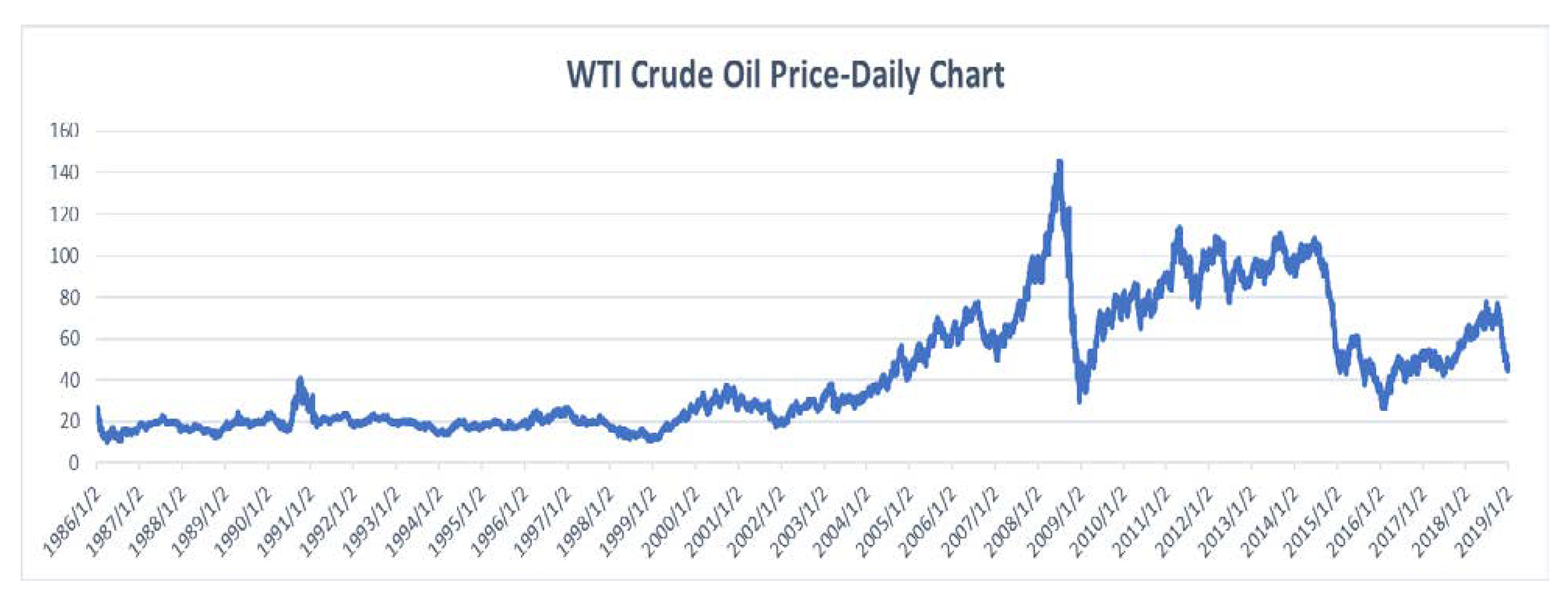
In this section, through a series of experiments, we verified the proposed CEEMDAN-ML-GRU model is more advanced than the state-of-the-art methods, which include the EEMD-LSTM. In order to measure and compare the forecasting performance of different models, WTI crude oil prices is employed for the sample data set for the experiment. This dataset source is the U.S. Energy Information Administration (EIA; http://www.eia.doe.gov/) and has 8321 observations that include all daily data from 2 January 1986 to 3 January 2019. A test set with 1664 observations is used to evaluate the prediction performance. The daily chart of WTI crude oil prices is illustrated in Figure 6.

4.2. Evaluation Metrics and Baselines

Following, we adopt three metrics including the root mean squared error (RMSE), mean absolute percent error (MAPE) and Diebold-Mariano (DM) to evaluate our model.

(1) Root mean squared error (RMSE):

$$\mathrm{RMSE}(y,\hat{y})=\sqrt{\frac{{\sum }_{i=1}^N{(y_i-{\hat{y}}_i)}^2}{N}}$$

(22)

RMSE is one of the most common metrics and often used to measure the deviation between observations and prediction in the task of machine learning models. The letter y in the formula above denotes the observations, $\hat{y}$ is the prediction, and N indicate the number of samples.

(2) Mean absolute error (MAE):

$$\mathrm{MAE}(y,\hat{y})=\frac{{\sum }_{i=1}^N|y_i-{\hat{y}}_i|}{N}$$

(23)

(3) MAE can better reflect the actual situation of the error of prediction. Mean Absolute Error Percentage (MAPE):

$$\mathrm{MAPE}(y,\hat{y})=\frac{1}{N}{\sum }_{i=1}^N\left|\frac{y_i-{\hat{y}}_i}{y_i}\right|$$

(24)

MAPE measures not only the absolute error between the predicted value and the observations, but also the relative distance. Unlike the previous two metrics, MAPE stands for percentage error, which can help it compare errors between different data sets.

(4) Diebold-Mariano Test (DM test):

$$\mathrm{DM}=\frac{\overline{d}}{\sqrt{\left[{\gamma }_0+2{\Sigma }_{k=1}^{h-1}{\gamma }_k\right]/n}}$$

(25)

It is used to test the statistical significance of the forecast accuracy of two forecast methods. Variable d is the subtraction of absolute error of the two methods. $\overline{d}$ is the mean of d_i. ${\gamma }_k$ is the autocovariance at lag k. DM ∼ N(0, 1), if the p-value > α, we conclude there is no significant difference between the two forecasts.

An ideal metric is not only reflected in the description of prediction accuracy, but also required to reflect the distribution characteristics of errors. Because of their effectiveness, these metrics are widely used for error measurement in regression or prediction tasks. The definition of each metric is different. When the sample size is large enough, RMSE is more reliable. RMSE is more suitable for Gaussian distribution error measurement than MAE, and MAE has a better performance in measuring uniform error. A single metric is not enough to judge the pros and cons of the model. We need to combine multiple metrics to determine the pros and cons of the model [39].

To verify that the proposed method is advanced, we compare our method with a series of models, most of them mentioned in previous sections. These models include not only the common models such as: naïve forecasts(that the prediction is the same as the last period), ARRIMA, least squares SVR (LSSVR), ANN RNN, LSTM, but also some hybrid models such as: EEMD-ELM, EEMD-LSSVR, EEMD-ANN, EEMD-RNN, EEMD-LSTM and EEMD-SBL-ADD. Both EEMD-LSTM and EMD-SBL-ADD have been proposed in the last two years and represent the current state-of-the-art approaches for crude oil forecasting.

4.3. Experimental Settings

There is one input layer, two hidden layers of GRU and one dense layer in our proposed model. Figure 7 illustrate its Tensorflow computation graph which indicate the network architecture in our method. Each input sample is a matrix of n × m, which is represented by a NumPy array. ‘n’ is the lagging order and ‘m’ is the number of IMFs and residue. By trial and error, we determine set the number of hidden neurons to 32 and MSE as the loss function. The optimizer of training is adaptive moment estimation (Adam) which solve the problems of other algorithm, such as learning rate disappearing, convergence slowly or loss function fluctuating greatly. The learning rate in following experiment is set to 0.01. We adopt the strategy of one day ahead prediction to carry out our tasks. In other words, the prices of the past n days (p₁, p₂, … p_n−1, p_n) is used to predict the price of the (n + 1)th day. Letter n is called the lag order which related to the size of neuron of the GRU. We adopt a strategy of grid search to determine the number of lagging order that is important for time series analysis. By trial and error, the lag order was set to 32.

For comparison purposes, we set the same initialization parameters for several deep learning models that participated in the experiment. For other parameters, since they have little effect on the results, we set the parameters to default.

The methods mentioned in the previous literature will be compared to our introduced approach in the performance of crude oil prices forecasts. These methods include not only the single model, LSSVR, ANN, ARIMA, and LSTM, but also the hybrid method EEMD-LSTM, which is considered the state-out-of- art method in crude oil prices forecasting.

In this study, all experiments are conducted in Python 3.7 via several specialized package, such as TensorFlow-GPU 2.0, Pyeemd 1.4, Keras 2.3 and so on. All experiments are conducted on a PC with a 3.2 GHz CPU, 16 GB RAM and 12 GB CG card.

4.4. Experimental Process, Result and Analysis

4.4.1. Data Decomposition

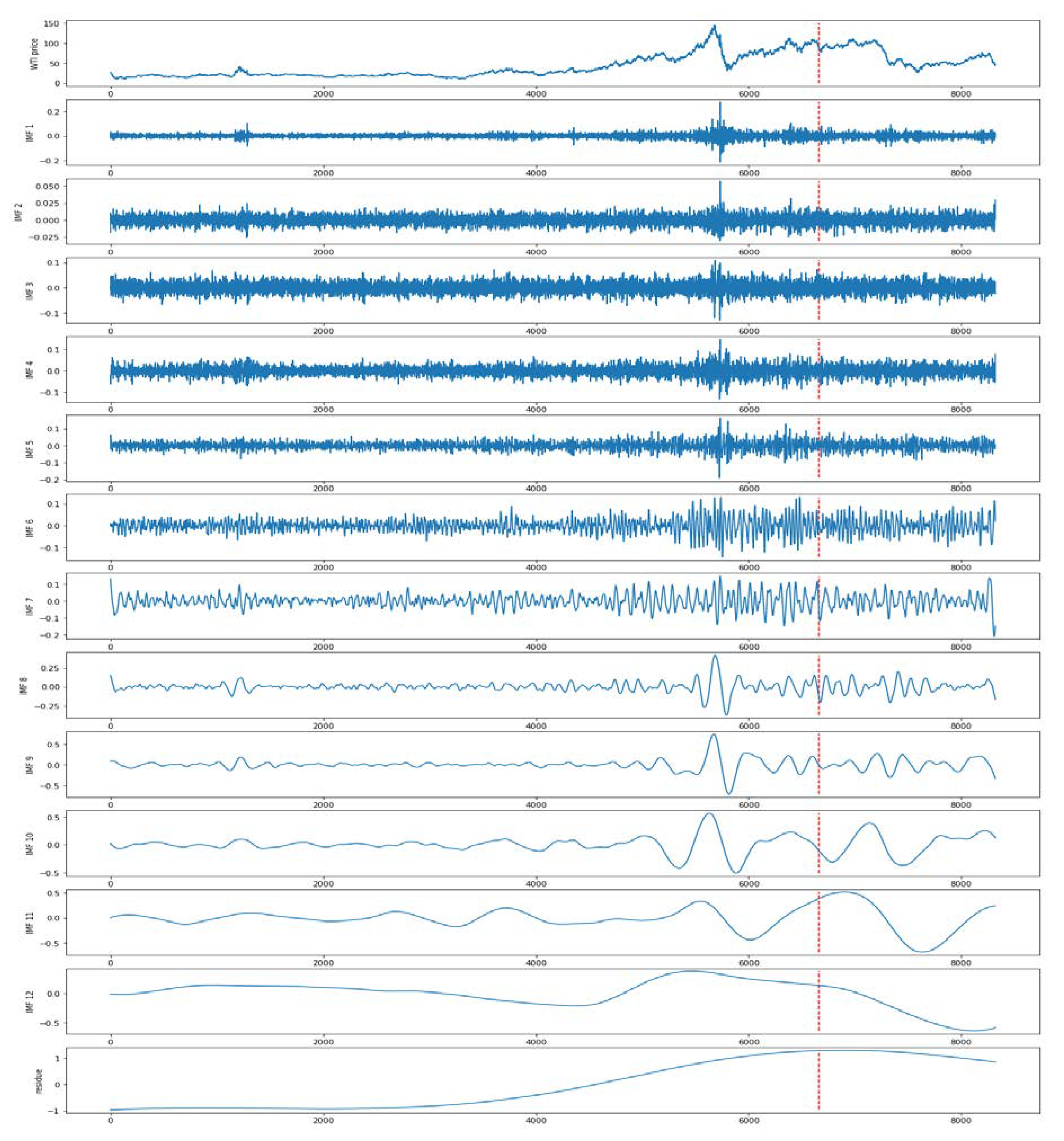
The original WTI crude oil is decomposed to 13 components which include 12 IMFS and one CEEMDAN residue, where we added the white noise with standard deviation of 0.01 and the number of ensemble size is equal to the size of dataset. Then the IMFs and residue are splinted into the train set and test set. Both them are illustrated in Figure 8, in which the left part of dotted line is train set and the right part is test set.

By trial and error, we determine the parameters of ensemble size of 0.05 and noise strength of 100. It means that the white noise data with standard deviation of 0.05 and quantity of 100 will be added to the original data. Before data decomposition, we initialize the other parameters of the algorithm.

Table 1. EEMD and CEEMDAN parameters description.

Parameter	Description
spline_kind	Defines type of spline, which connects extrema
nbsym	Number of extrema used in boundary mirroring
max_imf	IMF number to which decomposition should be performed
ensemble_size	Number of trials or EMD performance with added noise
noise_strength	Standard deviation of the additional noise.

shows the names and descriptions of the main parameters.

Table 2. Parameters settings.

Method	Nbsym	Max_imf	Trials	Noise_Width/Epsilon
EEMD	2	ALL	100	0.05
CEEMDAN	2	ALL	100	0.05

shows the parameter settings.

The time–frequency spectra of IMFs and the residue by CEEMDAN after decomposition are shown in Figure 8. We divide the original data and the decomposed result into a training set and a test set. The former accounts for 80% of the entire dataset, and the latter accounts for the remaining 20%. As shown in Figure 8, the data on the left side of the dotted line constitutes the training set, and the test set is on the right. As one kind of supervised learning algorithm, the input paired to the desired output in both the training and test sets.

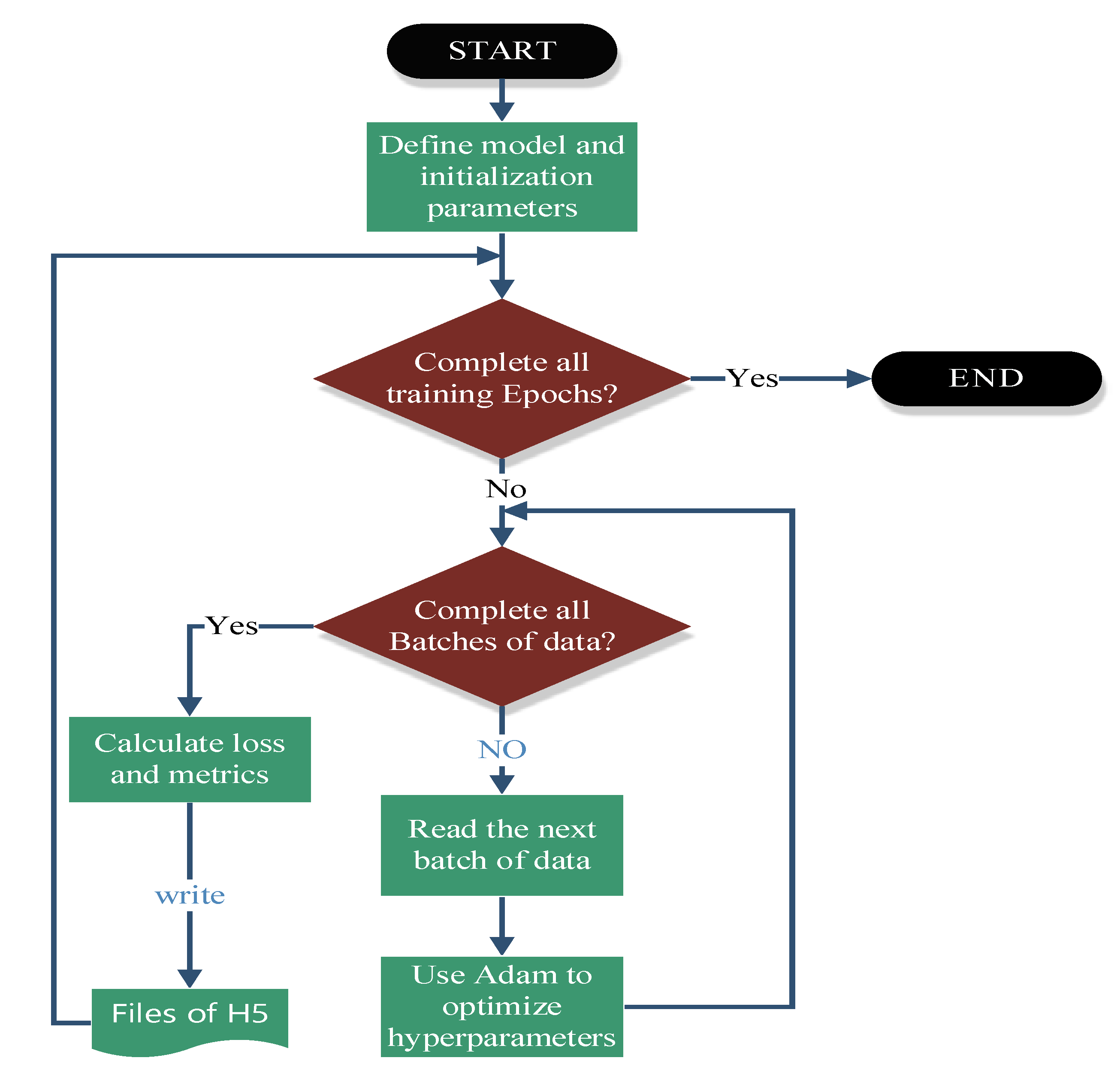
4.4.2. Training/Learning

After the model is build, we move on to the next step: training/learning. In this process, the training data is continuously feed into the model to incrementally improve the model’s predictive performance. Both the loss function and optimizer of adaptive moment estimation (Adam) mentioned earlier are used to evaluate and optimize the model in training to achieve the purpose of model optimization. The workflow of training as shown in Figure 9.

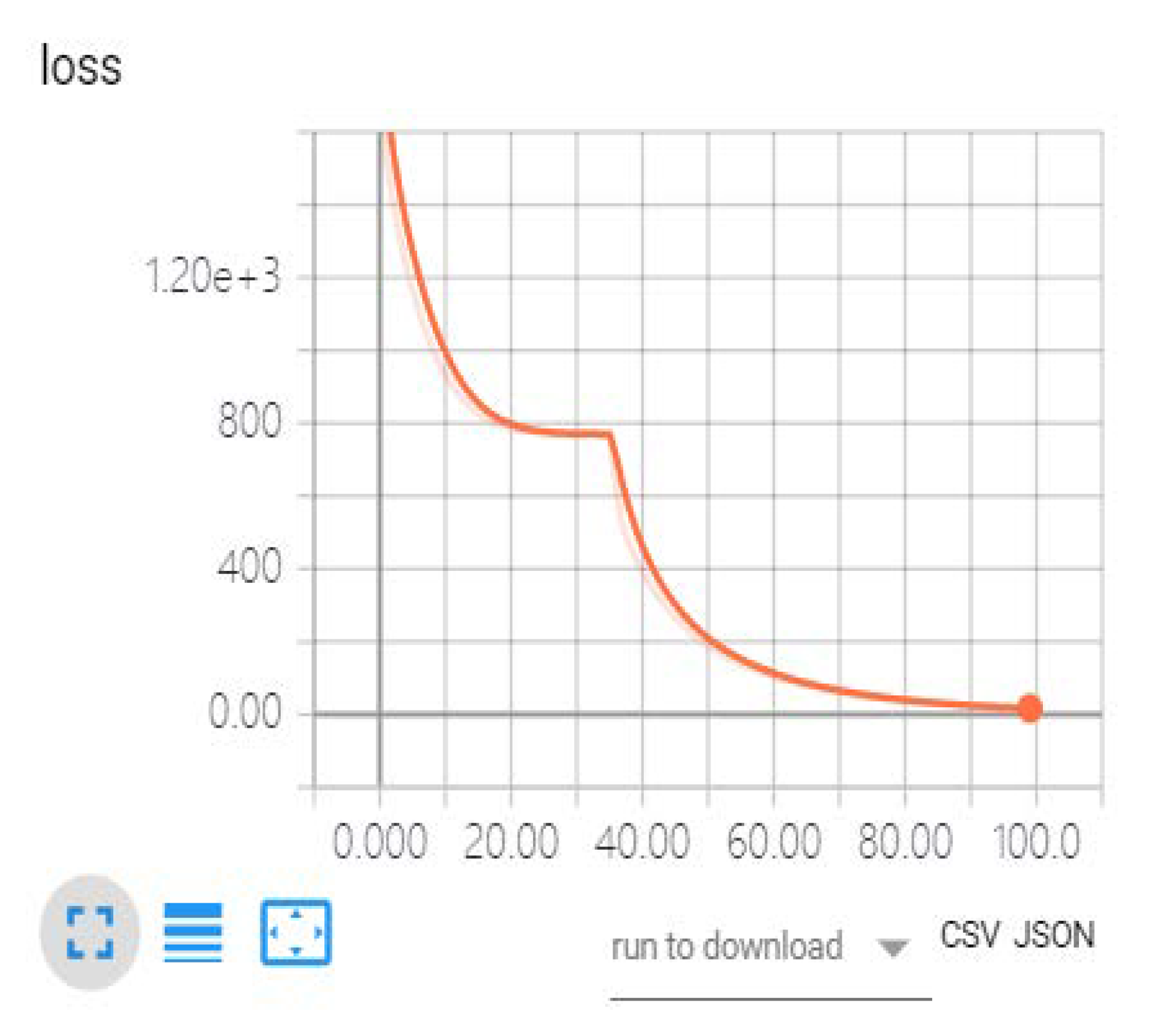
The trend of the loss function curve during the iteration of model training from 1st to 100th epoch is shown in the Figure 10.

The optimization algorithm mentioned above determines the optimization efficiency of the model, while loss represents the distance between the prediction and the observation. From the preceding graph, we observe that the loss curve descends rapidly in the initial epochs of training iteration, which shows that the model is optimized significantly by tuning the hyperparameter. However, between the 25th and 35th epochs of training, the loss curve is flat due to adaptive adjustment of the learning rate. After that, the curve continues to descend rapidly. The curve descending slowly means that loss saturated after 70 epochs of iterations. After 100 training epochs, the loss (MSE) has descended to a very low level. In fact, we conducted 2500 epochs experiment for each model, with 120 samples per batch. Once the training\learning of the hyperparameters (weight) in the model is completed, the model can be used in the tasks of crude oil price forecasts. The experimental results are shown later in the paper.

4.4.3. Predictive Performance of Different Single Model

We propose a hybrid model that includes two components, a decomposition algorithm CEEMDAN and a prediction model Multi-layer GRU. In order to make the method evaluation more accurate, we adopt a combination of independent evaluation and overall evaluation. So, we expand single model comparison and hybrid model comparison between two sets of experiments.

Here, we will evaluate our proposed CEEMD-ML-GRU’s effectiveness for improving forecasting accuracy. The compared single models included the naïve forecasts, one classical time series method of ARIMA, two famous machine models of LSSVR and ANN and two popular deep learning model of LSTM and GRU. The samples used in each iteration of the deep learning model are randomly drawn, which makes the results of each prediction different. In order to improve the robustness of the model, experiments with each parameter condition were required to be trained 100 times. In order of performance, the metric at the median position represents the model. The results are shown in

Table 3. Predictive performance comparison of single methods.

Metrics	Methods
	ML-GRU	GRU	LSTM	LSSVR	ANN	ARIMA	Naive
RMSE	1.2869	1.4820	1.4818	1.6473	1.5223	2.4861	1.5336
MAE	1.2424	1.3817	1.3788	1.5219	1.3649	2.2134	0.9271
MAPE	0.0138	0.0152	0.0153	0.0168	0.0156	0.0268	0.0152

.

From Table 3,

Table 4. Comparison of GRU and LSTM model in the number of parameters.

Method	Input Shape	Output Shape	Total Params
GRU	(32, 13)	(32, 32)	4416
LSTM	(32, 13)	(32, 32)	5888

and

Table 5. The Diebold–Mariano (DM) test results for single models on WTI crude oil prices.

DM Test	Benchmark Model
	GRU	LSTM	LSSVR	ANN	ARIMA	Naive
ML-GRU	−2.1644 (0.02365)	−2.319 (0.02017)	−15.6146 (0.0000)	−3.4532 (0.0000)	−20.198 (0.0000)	−2.1581 (0.02517)

, we can see that:

(1)

Among all these models, the multi-layer GRU (ML-GRU) stacking network performed the best on the metrics of RMSE and MAPE. As shown in Table 5, ML-GRU significantly outperformed higher prediction accuracy than other single models. This phenomenon further illustrates that the multi-layer neural network can be used to solve complex issues.

(2)

Both GRU and LSTM, designed for long term dependencies of time series show better performance than other traditional machine learning models for crude oil price forecasts. From Table 3, we observe that there is no significant difference between the LSTM and GRU models in the task of crude oil price prediction. Table 4 indicates that GRU has higher efficiency than LSM, because GRU network needs 30% less hyperparameters that need be learned than LSTM, during the training process. It means that GRU neural network use less training parameters comparing to LSTM, and therefore use less resources of computing and storage, execute faster and train faster than LSTM’s.

(3)

It is interesting that the comprehensive score of the naive forecasts surpasses classical methods such as ARIMA, ANN and LSSVR, and even achieve the best score on MAE. This phenomenon indicates that the complex crude oil price trends are difficult to predict. Misuse of some models, the result is even worse than doing nothing.

(4)

While ARIMA performed the worst. The results further confirm that ARIMA, a classic time series analysis model, doesn’t perform well at issues of nonlinear and non-stationary time series.

4.4.4. Effect of Selecting Different Hybrid Approaches

On the basis of the previous single model prediction, we continue to evaluate the performance of the hybrid model based on the decomposition method.

Table 6. The experimental results in terms of hybrid approaches on WTI crude oil prices forecasting.

Metrics	EEMD			CEEMDAN
	RMSE	MAE	MAPE	RMSE	MAE	MAPE
ML-GRU	0.9619	0.9341	0.00987	0.9276	0.9134	0.0094
GRU	0.9912	0.9719	0.0106	0.9334	0.9278	0.0101
LSTM	0.9862	0.965	0.0104	0.9329	0.9261	0.0099
LSSVR	1.1265	1.0847	0.0116	1.1197	1.0903	0.0114
ANN	1.0508	1.0121	0.0106	1.0476	1.0118	0.0105

shows the prediction performance of the corresponding hybrid models based on EEMD or CEEMDAN.

Table 7. The Diebold–Mariano (DM) test results for hybrid models on WTI crude oil prices.

Benchmark Model
DM Test	ML-GRU	EEMD-LSTM EEMD-ML-GRU CEEMDAN-LSTM CEEMDAN- GRU Naive
CEEMDAN-ML-GRU	−6.3309(0.0000)	−1.759(0.0776) −15.6146(0.0000) −3.4532(0.0000) −20.198(0.0000) −11.7541(0.0000)

demonstrates that the result of DM test between CEEMDAN-ML-GRU and the other two models.

In this set of experiments, we added a prediction model based on the EEMD decomposition algorithm, and these hybrid models have appeared in the latest literature. Each single model combines CEEMDAN and EEMD respectively, and thus two sets of mixed methods will be obtained. Subsequently, these models were tested in the WTI crude oil price prediction task to derive who is the optimal model. Table 6 demonstrates the predictions of different hybrid models. From the Table 6 and Table 7, we can observe that:

(1)

Both EEMD and CEEMDAN plus prediction models outperform single model significantly in this prediction task. It indicates that machine learning models with signal processing algorithm based contribute to the better forecasting performance in the nonlinear and non-stationary time series analysis.

(2)

The hybrid model based on CEEMDAN has better prediction accuracy than that based on EEMD’s. The residual noise from the components decomposed by EEMD, cause a certain extent of reconstruction error, and affect the overall predictive accuracy ultimately.

(3)

The ML-GRU with multi-layer architecture still performs better than the GRU with single-layer architecture on the decomposed data. CEEMDAN-ML-GRU, our proposed method has been verified to the best method for the task of crude oil price forecasting.

5. Conclusions

In this study, a hybrid model called CEEMDAN-ML-GRU for crude oil price forecasting is proposed. This model takes full use of the advantages of the signal processing algorithm CEEMDAN and the multi-layer gated recurrent unit networks (ML-GRU). As mentioned in the previous section, the hybrid model uses CEEMDAN to solve the non-stationarity problem of crude oil price data, and generalizes the nonlinear crude oil prices data by a multi-layered GRU neural network. We conduct a large number of experiments to verify the effect of the proposed method in forecasting task by using the WTI price data as sample data. The experimental results show that our proposed method goes beyond other traditional statistical methods, machine intelligent algorithms and other hybrid models, which include the EEMD-LSTM method proposed in 2019.

In addition to crude oil price forecasts, the introduced CEEMDAN-ML-GRU model can also be extended to solve other complex problems in other areas, such as time series forecasts or risk measurements in financial markets. The main purpose of this approach is to improve the accuracy of short-term crude oil price predictions and help decision makers minimize the risks of the crude oil market. However, the proposed method is mainly applied to short-term forecasts, so only daily data is used. If we need to predict long-term price trends, we need to combine this method with economic theory or measurement methods to play a greater role. This is exactly the research plan that we will follow in our future research.