Numerical Investigation of Vertical Crossflow Jets with Various Orifice Shapes Discharged in Rectangular Open Channel

Abstract

Vertical jet in flowing water is a common phenomenon in daily life. To study the flow and turbulent characteristics of different jet orifice shapes and under different velocity ratios, the realizable k-ε turbulent model was adopted to analyze the three-dimensional (3D) flow, turbulence, and vortex characteristics using circular, square, and rectangular jet orifices and velocity ratios of 2, 5, 10, and 15. The following conclusions were drawn: The flow trajectory of the vertical jet in the channel exhibits remarkable 3D characteristics, and the jet orifice and velocity ratio have a significant influence on the flow characteristics of the channel. The heights at which the spiral deflection and maximum turbulent kinetic energy (TKE) occur for the circular jet are the smallest, while those for square jets are the largest. As the shape of the jet orifice changes from a circle to a square and then to a rectangle, the shape formed by the plane of the kidney vortices and the region above it gradually changes from a circle to a pentagon. With the increase in the velocity ratio, the 3D characteristics, maximum TKE, and kidney vortex coverage of the flow all gradually increase.

1. Introduction

In real life, it is a typical vertical jet that pollutants such as waste gas and wastewater enter the river through the riverbed. After entering the water, the pollutants can have a good or bad impact on the water environment. The study of vertical jets is of great significance for pollutant diffusion, sediment transport, and water temperature regulation.

When a high-velocity flow is ejected from a pipeline into a low-velocity water environment, a vertical jet is formed. In recent years, different researchers have conducted numerous studies on the flow characteristics and pollutant diffusion characteristics when there is a vertical jet in flowing water [1,2,3,4,5]. Scorer [6] is arguably the first person who noticed the presence of a counterrotating vortex in a vertical jet. He pointed out that a pair of counterrotating kidney vortices exist in the channel when a small circular orifice emits a high-velocity flow. In recent years, many scholars have conducted extensive research on vertical jets under different conditions from physical experiments [7,8] and numerical simulations [9,10,11], but the existing research is mainly focused on circular jets. Smith and Mungal [12] employed a planar laser-induced fluorescence technology (PLIF) technique to divide the flow field under the condition of a circular hole jet in a wide range of 5 to 25 into three parts and analyzed the kidney vortices and their attenuation characteristics. Based on the relevant experimental data of momentum transport and the turbulence characteristics of a circular vertical jet, Wang and Law [13] proposed a second-order integral model to analyze the turbulence characteristics of a vertical jet. The data calculated by Huai et al. [14] using the k-ε turbulent model are in good agreement with Andreopolous and Rodi [15] test data. Zhu and Shin [16] used different turbulent models to analyze the flow characteristics of water flow under co-current jet conditions and found that the simulation results of renormalization group (RNG) k-ε and realize k-ε are significantly better than the standard k-ε, and the difference between the calculation results of k-ε and realize k-ε is small. Zeng and Huai [17] analyzed the flow field structure and bifurcation phenomenon of a thermal buoyant jet under the condition of a circular hole vertical jet using the finite analysis method based on the RNG k-ε turbulence model. Large eddy simulation (LES) [18] and Scale adaptive simulation (SAS) [19] can also realize relevant research of the vertical jet.

Although circular orifice jets are the most common in practice, they are not unique. The change in the shape of the jet orifice can affect the flow trajectory and energy conversion of the jet. Therefore, it is necessary to study the shape of the jet orifice, but there are few studies on this aspect. Haven and Kuroska [20] adopted the laser-induced fluorescence (LIF) technique and particle image velocimetry (PIV) in a top-down jet experiment with a small velocity ratio range of 0.4 to 2.0 and found that the square and rectangular jets can also produce kidney vortices, and the change in the jet orifice shape affects the local shape of downstream vortices. Due to the limitation of the accuracy of the physical experiment, the trajectory and turbulent characteristics of the jet in the water have not been thoroughly studied due to the change in the shape of the jet orifice. However, the vortex structure due to buoyancy in the process of jet from top to bottom and jet from bottom to top is also different.

The trajectory of the jet deflects, which moves along the direction of the open channel while rising, due to the influence of the original flowing water in the open channel when the jet flows from the riverbed into the open channel environment. The velocity of the jet beam in the channel is a combination of its vertical upward velocity and the original horizontal velocity of the water in the channel. The trajectories and other effects of the jet beam in the closed and open channel are different due to the different velocity distributions along the water depth, especially at a large velocity ratio. In this paper, we choose a smaller range of velocity ratio to study the vertical jet in an open channel.

In order to further investigate the jet trajectory and turbulent characteristics with various jet orifice shapes, this paper analyzes the 3D flow structure, turbulent kinetic energy, and vortex of circular, square, and rectangular jet orifices in a wide range of velocity ratios of 2, 5, 10, and 15, respectively. This research complements the lack of research on different jet orifice shapes under vertical jet conditions, and can provide basic guidance for pollutant diffusion, water temperature regulation, and sediment transport in the river.

2. Materials and Methods

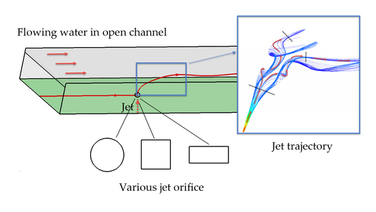
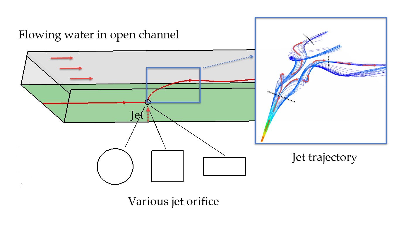
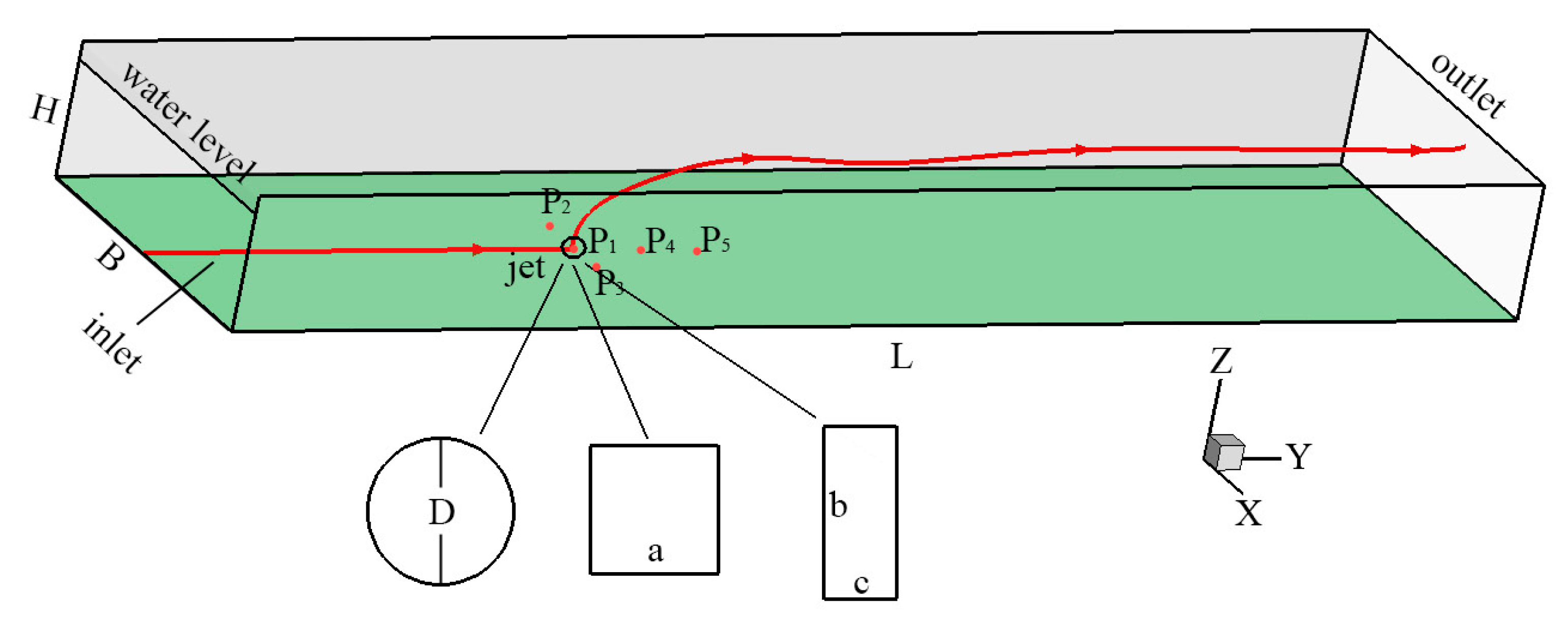
2.1. Model Layout

The model built in present work is a straight channel with a rectangular cross-section, the length (L), width (B), and height of which are 3 m, 0.8 m, and 0.3 m, respectively (shown in Figure 1). The water depth (H) at the inlet is 0.26 m and the distance between the center of the jet outlet, placed at the bottom of the model, to the inlet is 1 m. To study the influence of the jet orifice shape on the flow and turbulence characteristics of the straight channel, the shape of the jet orifice was set to be circular, square, and rectangular while maintaining the same jet orifice area and average flow velocity. The circular diameter is D = 5 mm, the square side length is a = 4.43 mm, and the rectangular outlet has a side length ratio of b/c = 2, where b and c are the dimensions along the width and length directions respectively, of the channel. The average velocity, u₀, at the inlet is 0.0826 m/s, the average velocity at the jet outlet is u_j, and the velocity ratio is calculated using Equation (1). Different velocity ratios of 2, 5, 10, and 15 are adopted to analyze the influence of the jet orifice shape on the channel under different velocity ratios (listed in

Table 1. Parameters of different cases.

Series	Shape	B	H	L	u0	D	a	b	c	uj	r	Rej	Cells
		(m)	(m)	(m)	(m/s)	(mm)	(mm)	(mm)	(mm)	(m/s)
Case 1	Circular	0.8	0.3	3	0.0826	5	-	-	-	0.165	2	924	703,080
Case 2	Circular									0.413	5	2312	703,080
Case 3	Circular									0.826	10	4625	703,080
Case 4	Circular									1.23	15	6887	703,080
Case 5	Square					-	4.43	-	-	0.165	2	924	703,080
Case 6	Square									0.413	5	2312	703,080
Case 7	Square									0.826	10	4625	703,080
Case 8	Square									1.23	15	6887	703,080
Case 9	Rectangular					-	-	6.26	3.13	0.165	2	924	698,040
Case 10	Rectangular									0.413	5	2312	698,040
Case 11	Rectangular									0.826	10	4625	698,040
Case 12	Rectangular									1.23	15	6887	698,040

). Re_j, calculated using Equation (2), is the Reynolds number of the jet hole. In the present work, the center of the jet orifice is set as the origin of the coordinates, the flow direction is the positive direction of the Y axis, the positive direction of the X axis is determined using the right-hand rule, and the positive direction of the Z axis is vertical upward.

$$r=u_{\mathrm{j}}/u_0$$

(1)

where r is the velocity ratio.

$$R{e}_j=\rho u_j\mathrm{D}/u_0$$

(2)

where Re_j, u_j, and D are the Reynolds number, velocity, and diameter of the jet hole respectively, and ρ and u₀ are the density and dynamic viscosity of the water, respectively.

2.2. Governing Equations

The realizable k-ε turbulent model proposed by Shih et al. [21] is adopted in this paper. This model is optimized on the basis of the standard k-ε turbulent model and can accurately simulate the jet flow, especially in terms of strong streamtrace bending, vortex, and rotation. The governing equations are as follows:

Continuity equation:

$$\frac{\partial \rho }{\partial t}+\frac{\partial (\rho u_i)}{\partial x_i}=0$$

(3)

Momentum equation:

$$\frac{\partial \left(\rho u_i\right)}{\partial t}+\frac{\partial \left(\rho u_i{u}_j\right)}{\partial x_j}=-\frac{\partial p}{\partial x_i}+\frac{\partial }{\partial x_j}\left[(\mu +{\mu }_t)\times (\frac{\partial u_i}{\partial x_j}+\frac{\partial u_j}{\partial x_i})\right]$$

(4)

Turbulent kinetic energy (k) equation:

$$\frac{\partial \left(\rho k\right)}{\partial t}+\frac{\partial }{\partial x_j}\left(\rho u_{j}k\right)=\frac{\partial }{\partial x_j}\left[\left(\mu +\frac{{\mu }_t}{{\sigma }_k}\right)\frac{\partial k}{\partial x_j}\right]+G_k+G_b-\rho \epsilon -Y_M+S_k$$

(5)

Turbulent dissipation rate (ε) equation:

$$\frac{\partial \left(\rho \epsilon \right)}{\partial t}+\frac{\partial }{\partial x_j}\left(\rho u_j\epsilon \right)=\frac{\partial }{\partial x_j}\left[\left(\mu +\frac{{\mu }_t}{{\sigma }_{\epsilon }}\right)\frac{\partial \epsilon }{\partial x_j}\right]+\rho C_1{S}_{\epsilon }-\rho C_2\frac{{\epsilon }^2}{k+\sqrt{\mathsf{\nu }\mathsf{\epsilon }}}+C_{1\epsilon }\frac{\epsilon }{k}{C}_{2\epsilon }{G}_b+S_{\epsilon }$$

(6)

$$C_1=max\left[0.43,\frac{\eta }{\eta +5}\right]$$

(7)

$$\eta =\frac{Sk}{\epsilon }$$

(8)

$$S=\sqrt{2S_{ij}{S}_{ij}}$$

(9)

$$S_{ij}=0.5(\frac{\partial u_j}{\partial x_i}+\frac{\partial u_i}{\partial x_j})$$

(10)

$${\mu }_{\mathrm{t}}=\frac{\rho C_{\mu }{k}^2}{\epsilon }$$

(11)

where $G_k$ and $G_b$ are the turbulent kinetic energy values caused by the average velocity gradient and buoyancy lift, respectively. $Y_M$ is the contribution of the compressible turbulent wave expansion to the overall dissipation rate, ρ is the water density, t is time, υ is the turbulent kinematic viscosity coefficient, $u_i$ is the average velocity in the direction of i, ${\mu }_t$ is the turbulent viscosity, $C_{\mu }$, $C_{1\epsilon }$, $C_{2\epsilon }$, ${\sigma }_k$, and ${\sigma }_{\epsilon }$ are model constants with values of $C_{\mu }$ = 0.09, $C_{1\epsilon }$ = 1.44, $C_{2\epsilon }$ = 1.92, ${\sigma }_k$ = 1.0, and ${\sigma }_{\epsilon }$ = 1.3, and $S_k$ and $S_{\epsilon }$ are user-defined source items.

2.3. Solver Settings and Boundary Conditions

Fluent software is adopted and the volume of fluid (VOF) method proposed by Hirt and Nichols [22] in 1981 is used to solve the free surface tracking problem in multiphase flow. This method uses a volume fraction function, F (x, y, z), to describe the position and volume ratio of the gas and liquid phases. F (x, y, z, t) = 1 indicates that the calculation unit is full of liquid, and F (x, y, z, t) = 0 indicates that the calculation unit is full of gas. Therefore, when 0 < F (x, y, z, t) < 1, there must exist an interface between the water and gas phases. Accordingly, a difference method can be used to calculate the interface position and solve for the free surface. The equations for calculating the volume fraction function in the VOF method are as follows:

$$\frac{\partial F}{\partial t}+u_i\frac{\partial F}{\partial x_i}=0$$

(12)

$$\rho =F_w{\rho }_w+\left(1-F_w\right){\rho }_a$$

(13)

$$\mu =F_w{\mu }_w+\left(1-F_w\right){\mu }_a$$

(14)

where, ${\rho }_w$ and ${\rho }_a$ are the densities of water and gas respectively, ${\mu }_w$ and ${\mu }_a$ are the viscosity coefficients of water and gas respectively, and $F_w$ is the volume fraction of the liquid phase.

A transient solver is used for the calculation. Pressure-velocity coupling is calculated by adopting the SIMPLE pressure correction algorithm proposed by Patankar [23], and open channel flow is used for the VOF sub-models.

To save computation time and maintain calculation accuracy, the model is divided into five sections (shown in Figure 2). A fine mesh is used near the jet orifice location, and a relatively coarse mesh is used for locations near the inlet and outlet of the channel in the Y direction. The number of grids in the jet orifice is 4, and the total number of grids of the channel is 84 in the X direction. The number of grids is 30 in the Z direction. So, the layouts of the mesh of different jet orifices are (100 + 4 + 50 + 75 + 50) × 84 × 30, (100 + 4 + 50 + 75 + 50) × 84 × 30, and (100 + 2 + 50 + 75 + 50) × 84 × 30, respectively. The red line in Figure 2 is the grid of the jet orifice. The numbers of grids in different cases are shown in Table 1.

The velocity-inlet boundary or pressure-inlet boundary are adopted to the water part or the air part of the channel, respectively. The inlet velocity of the water in the channel is set to the average and the magnitude is 0.0826 m/s. The pressure outlet is set at the outlet and the air–water interface is standard atmospheric pressure. The material of side walls of the sink in Reference [24] are glass, which is set to a non-slip boundary condition and a standard wall function is used near the sidewalls.

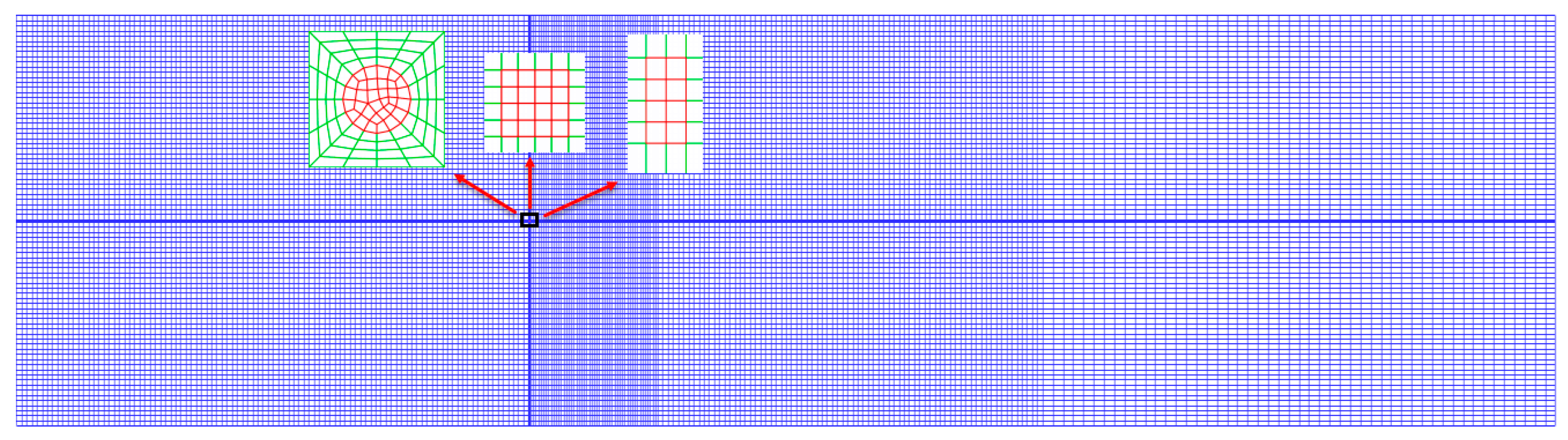
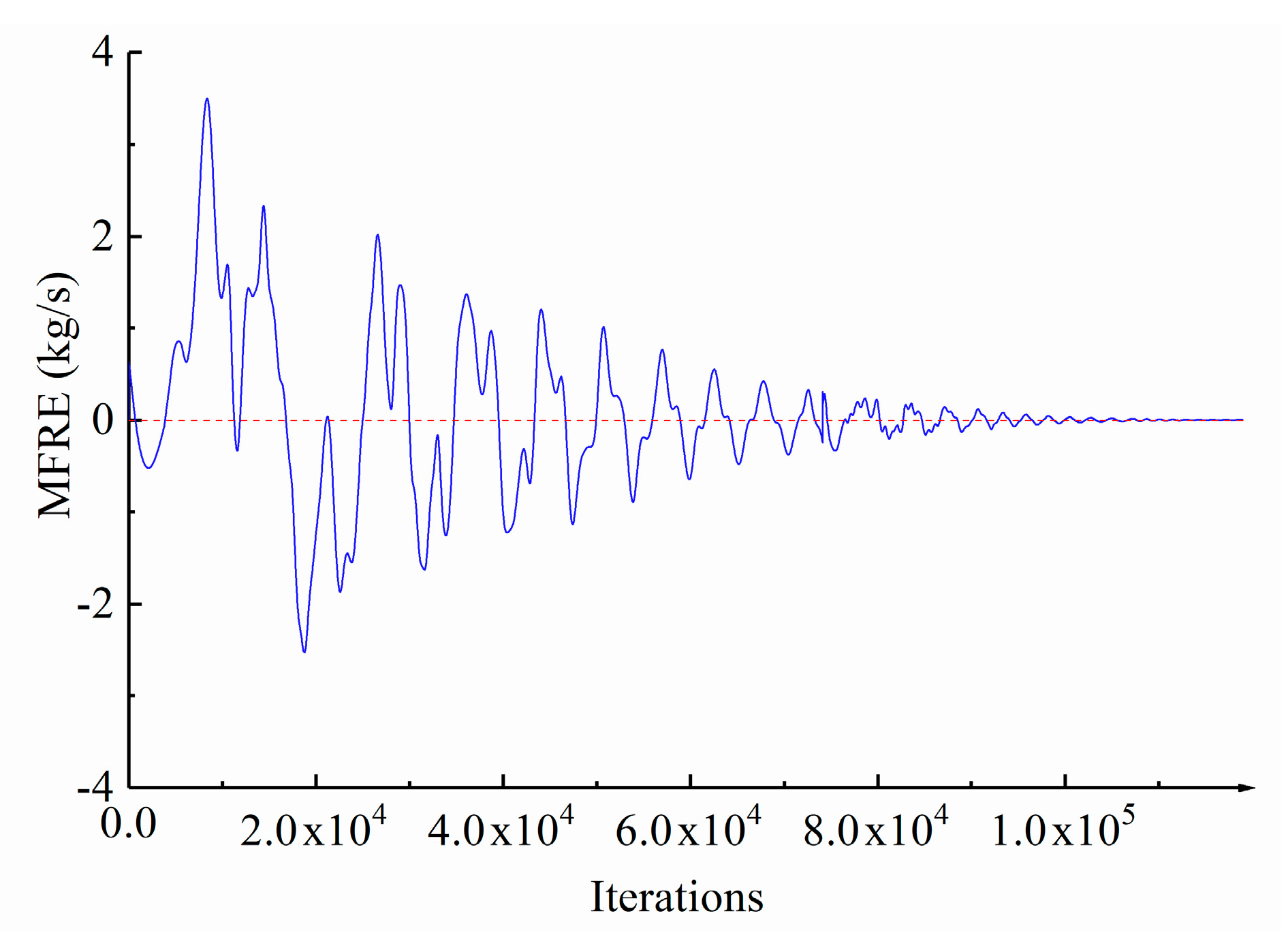
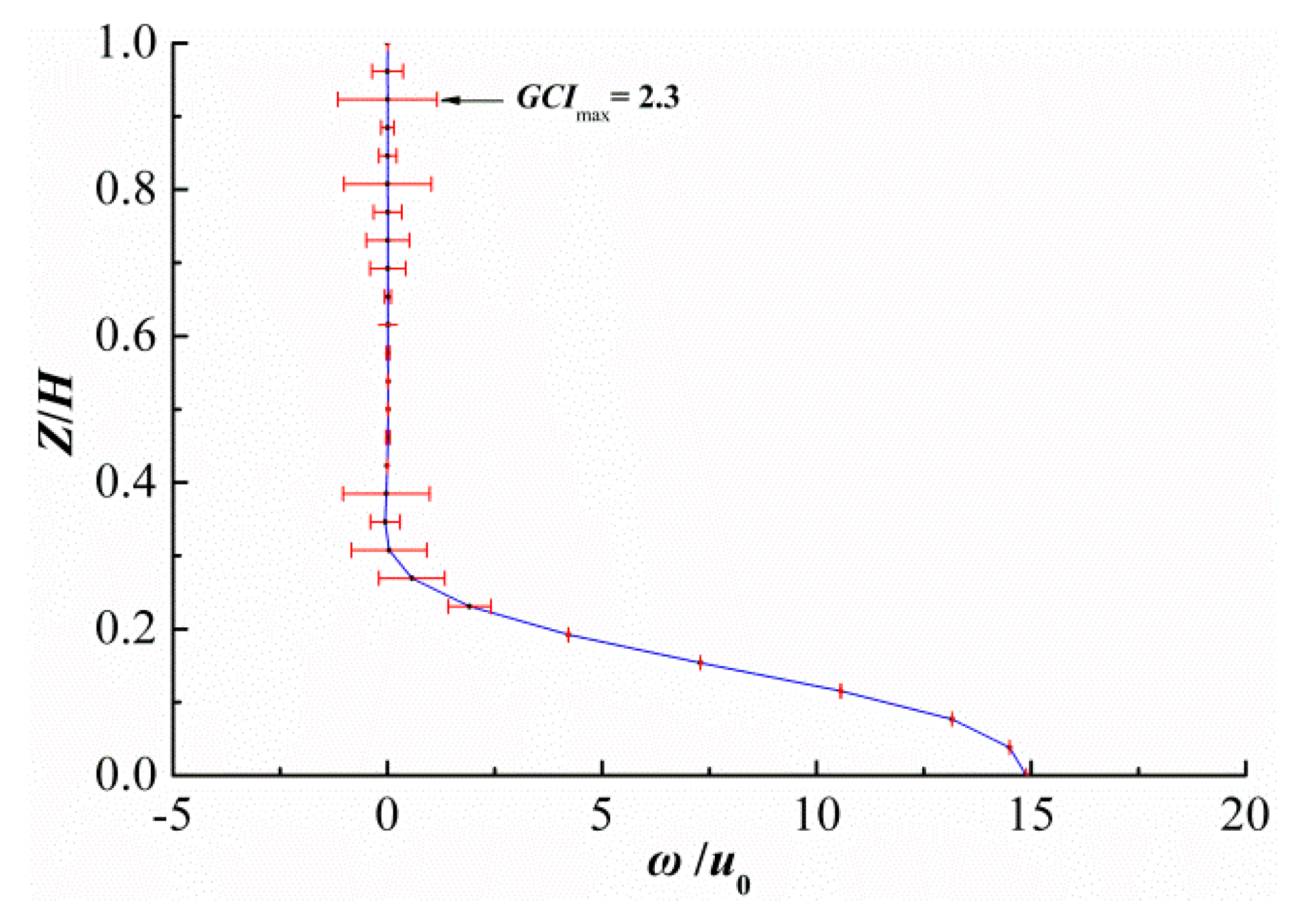
2.4. Convergence Stability and Mesh Sensitivity Analysis

The flow in the straight channel without a vertical jet is first calculated until it is steady, then its flow field is taken as the initial flow field for the channel with a vertical jet to carry out the relevant calculation. In the calculation, the mass flow rate error (MFRE) for the inlet and outlet of the channel are traced and the calculation is considered to be steady when the MFRE is small enough. To ensure the accuracy of the calculation, the vertical distribution of the velocity at the center of the jet orifice is compared at different times when the MFRE is relatively small. If the velocities are almost consistent, the calculation is considered to reach the final steady state required in this study. The time-history curve of the variation in the MFRE with the calculation time is shown in Figure 3, and the MFRE values of different cases are shown in

Table 2. MFRE values under different cases in steady state.

Title 1	Case 1	Case 2	Case 3	Case 4	Case 5	Case 6	Case 7	Case 8	Case 9	Case 10	Case 11	Case 12
MFRE (kg/s)	−0.006	−0.006	0.00002	0.007	0.002	0.01	−0.006	0.0004	−0.002	0.006	0.002	−0.001
Relative mass flow rate (%)	−0.36	−0.36	0.00	0.42	0.12	0.58	−0.35	0.02	−0.12	0.35	0.12	−0.06

.

For case 4, the grid convergence index (GCI) [25] of the velocity distributed vertically at the center of the jet orifice is calculated with the number of grids approximately equal to 0.54 million, 0.7 million, and 1.08 million to verify that the calculation in this study is independent of the meshing. The GCI is calculated as follows:

$$GCI=\frac{1.25\left|\frac{{\varphi }_1-{\varphi }_2}{{\varphi }_1}\right|}{{(h_2/h_1)}^P-1}$$

(15)

$$P=\frac{1}{\ln (h_2/h_1)}\left|\ln \left|({\varphi }_3-{\varphi }_2)/({\varphi }_2-{\varphi }_1)\right|+\ln (\frac{{(h_2/h_1)}^P-\mathrm{sgn}(({\varphi }_3-{\varphi }_2)/({\varphi }_2-{\varphi }_1))}{{(h_3/h_2)}^P-\mathrm{sgn}(({\varphi }_3-{\varphi }_2)/({\varphi }_2-{\varphi }_1))})\right|$$

(16)

where ${\varphi }_{\mathrm{i}}$ is the calculated value for the ith numerical grid with i = 1, 2, and 3, and $h_{\mathrm{i}}$ is the height of the first-layer grid of the ith numerical grid and satisfies $h_1$ < $h_2$ < $h_3$.

The variation in the vertically distributed GCI of the vertical velocity at the center of the jet orifice is shown in Figure 4, where ω is the vertical velocity. As shown in Figure 4, the maximum value of GCI is only 2.3, which indicates that the number of grids used in the present study (approximately 0.7 million) is appropriate.

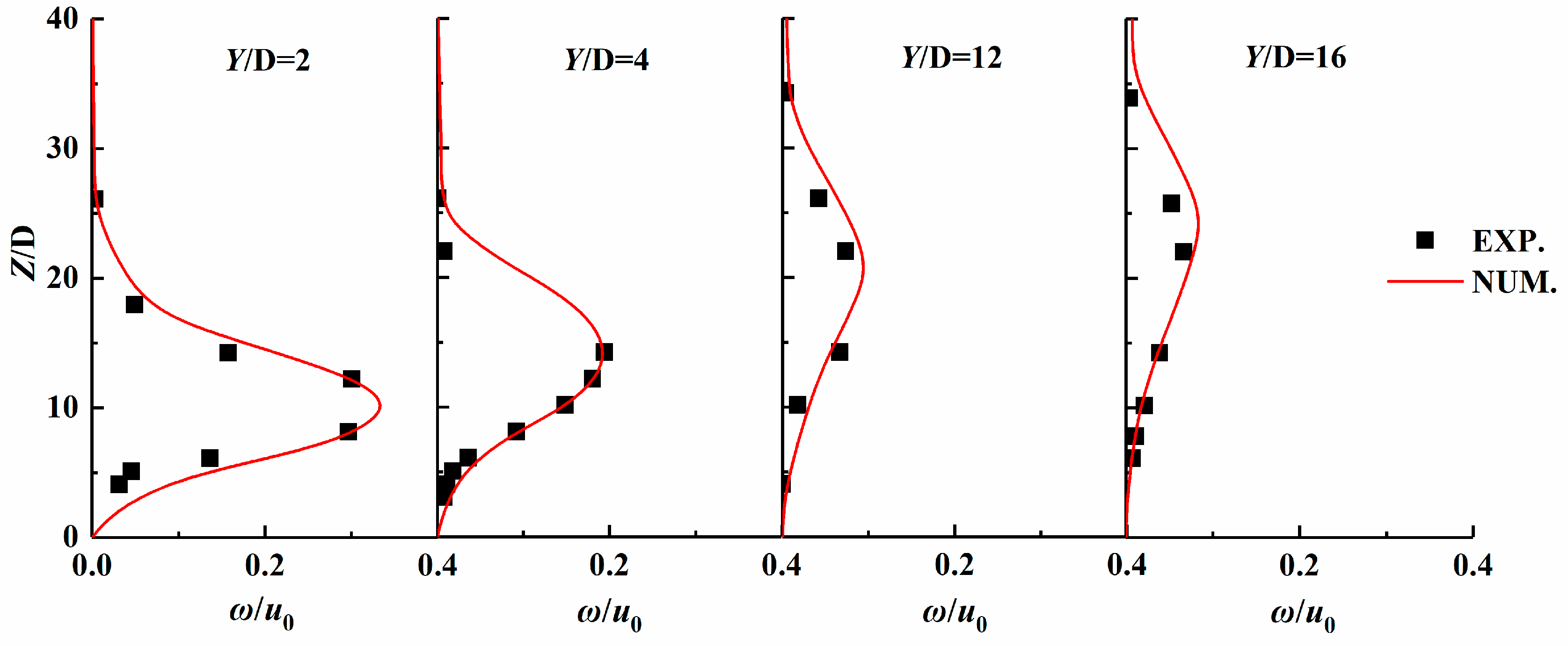
2.5. Numerical Model Validation

Before carrying out the study, it is necessary to conduct an accuracy analysis on the chosen numerical model to verify that it can meet the needs of this work. The calculation model selected in this study is from Reference [24], and the experimental water tank has a length of 15 m and a width of 4 m. The calculation and analysis in the present study show that the flow velocity of the water tank calculated using a 1:5 scale model is almost the same as that of the prototype. Therefore, to save calculation time, this scale is used for the width and length of the channel but the water depth in the original experiment and numerical model along the height direction is maintained at 0.26 m, the average velocity at the inlet of the straight channel is 0.0826 m/s, the jet outlet has a circular shape with a diameter of D = 5 mm, and the jet velocity ratio is 15. Using the center of the jet orifice as the coordinate origin, the numerical calculation results and the experimental data of the vertical velocities at the intersecting lines between the central plane face of the channel and the sections of Y = 2D, 4D, 12D, and 16D along the flow direction are selected and compared in Figure 5.

The comparison shows that the numerical calculation data are slightly larger than the experimental data at different positions. Considering that there may be a slight deviation in the positions in the actual measurement process of the physical experiment and that the vertical velocity at the middle sections is greater than that on the two sides, the numerical calculation results are considered to be in good agreement with the experimental results and can thus be used for further in-depth investigation in this study.

3. Results and Discussion

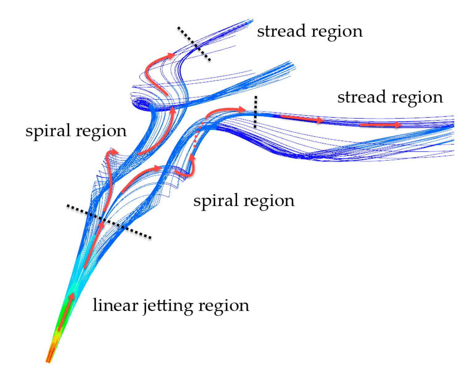
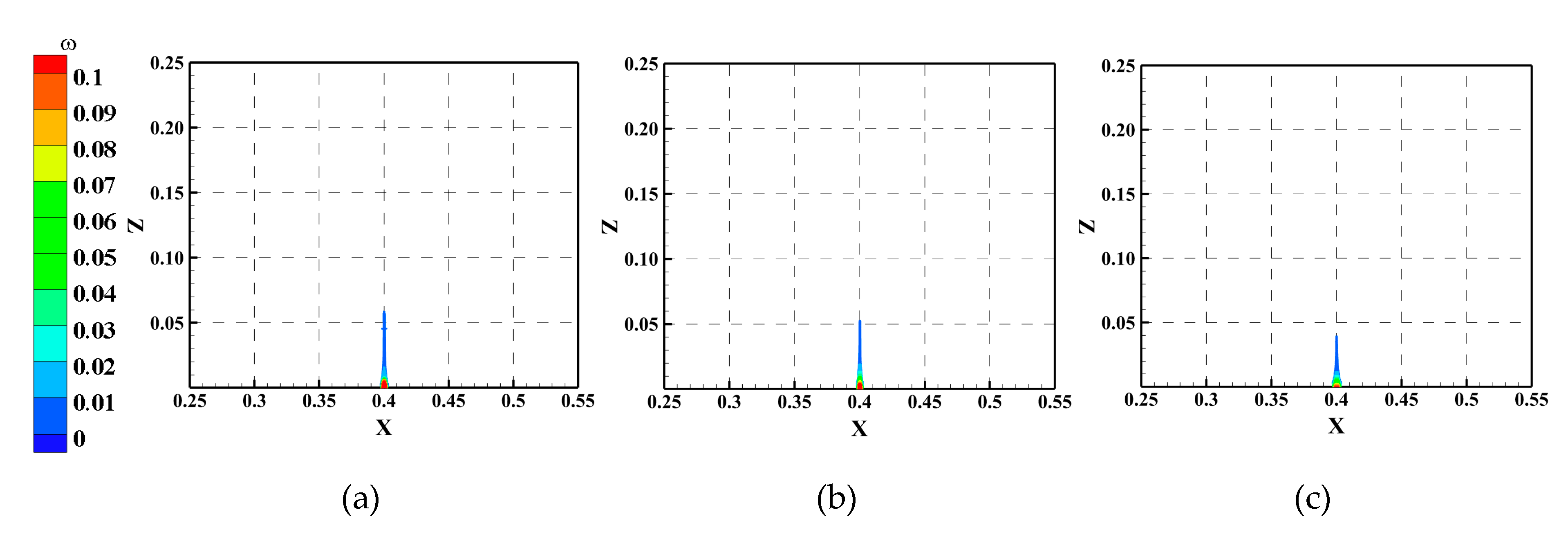
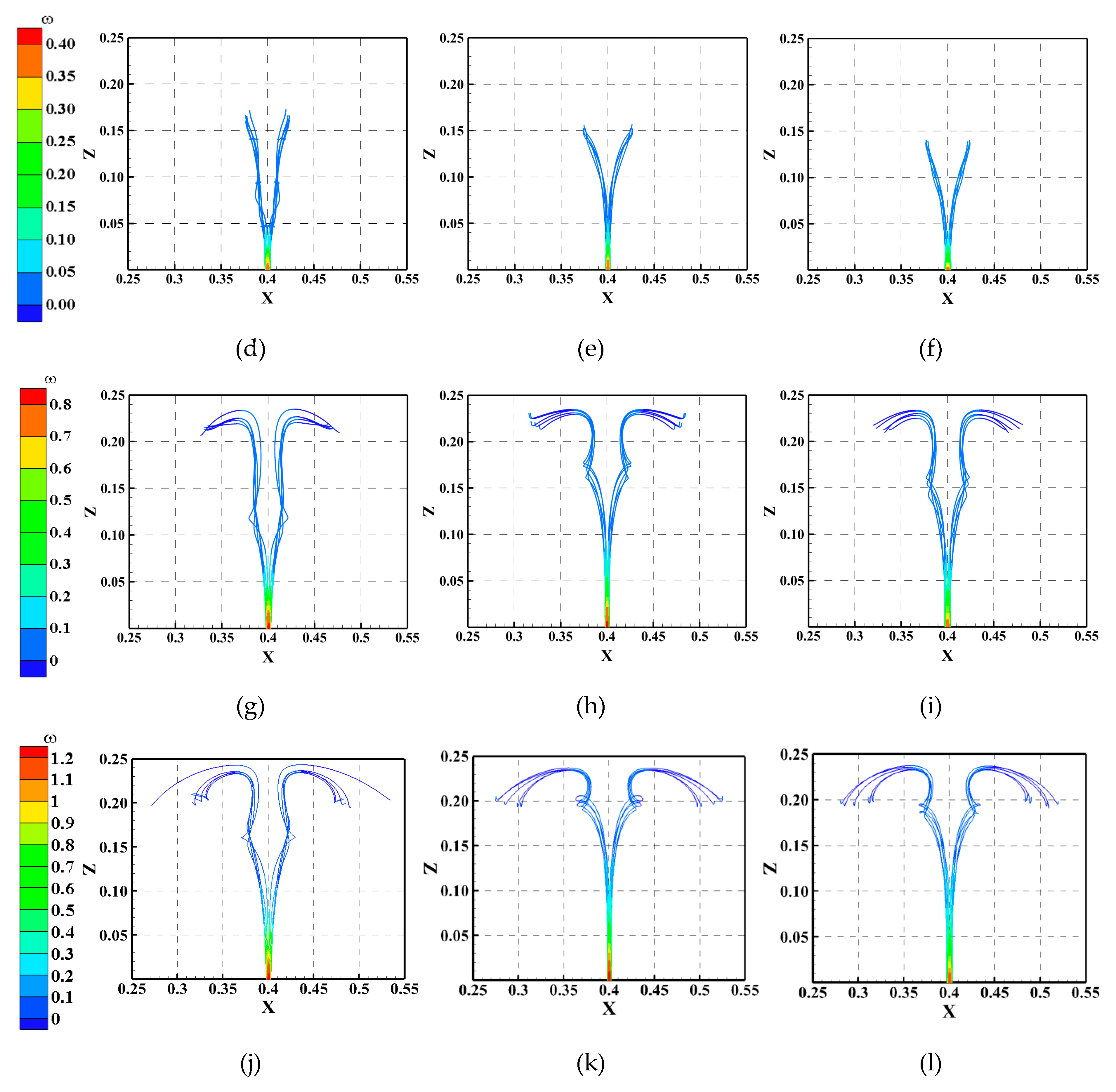
3.1. 3D Structure of the Flow Field

In the absence of the free surface flow, the jet behaves as a simple jet, with the fluid decelerating as it moves away from the jet exit. But the trajectory of the jet deflects, which moves along the direction of the open channel while rising, due to the influence of the original flowing water when the jet flows from the riverbed into the water environment flowing in the open channel. The jet beam successively undergoes three processes: linear jetting, spiral motion, and downstream steady linear motion (shown in Figure 6). When the flow is ejected rapidly from the orifice, the jet beam moves linearly. During the upward motion, the jet beam gradually increases due to the effect of gravity, the original flow field, and the absence of orifice constraints. When developed to a certain stage, the water with a high velocity in the middle of the jet orifice deflects significantly to move outward, which simultaneously drives the deflection of the surrounding water and forms a spiral flow due to the influence of the original water movement. After the energy is dissipated over a sufficiently long distance, the vertical velocity and spanwise velocity of the jet flow gradually decrease and eventually move downstream in line with the mainstream of the channel.

In this study, the trajectories of the jets with different orifice shapes and different velocity ratios at Y = 0 were analyzed, as shown in Figure 7.

As shown in Figure 7, when the velocity ratio is 2, the water is ejected from the orifice and then gradually draws closer toward the middle in the vertical direction, eventually forming a straight line without bifurcation. The shape of the jet orifice has a notable influence on the jet height and the jet height is the largest for the circular jet, followed by the square jet and then the rectangular jet. When the velocity ratio is 5, the jet beam bifurcates. The jet beams with circular and rectangular orifices bifurcate even when Z is less than 0.05 m, while the height at which the jet beam of the square orifice starts to bifurcate is relatively large, at more than 0.05 m. Further analysis reveals that the streamtrace line of the circular jet beam at the center of the orifice exhibits significant spiral deflection, while no apparent spiral deflection occurs in the jet beams with the other jet orifice shapes. When the velocity ratio is 10, there are two significant jet deflections in all the jet beams regardless of the orifice shape. The height at which the jet beam exhibits the first notable spiral deflection is the smallest for the circular jet beam, followed by the rectangular jet and then the square jet. For each of the three orifice shapes, the amplitude of the second deflection of the jet is significantly larger than that of the first deflection. After the second deflection, the streamtrace lines of the jets from the circular and rectangular orifices move vertically downward and then tend to stabilize and move downstream. After the second deflection, the jet beam with the square orifice exhibits a third deflection but with a smaller amplitude, and then tends to stabilize and move downstream. When the velocity ratio is 15, the variation in the jet beam trajectory for each of the three orifice shapes is similar to that with a velocity ratio of 10, although the amplitude of the second deflection has a large decrease in the vertical direction and all three exhibit third deflections. Based on the analysis of the influence in the Y direction, the circular jet beam has the largest influence range, while the rectangular jet beam has the smallest influence range.

An analysis of the cases with different velocity ratios shows that as the velocity ratio increases, the jets on the two sides first gather toward the center and gradually bifurcate; then, a spiral deflection occurs, and the number of occurrences continuously increases. The circular jet has the largest jet height, the smallest vertical height at which a spiral deflection occurs, and the largest influence range. The square jet has the largest vertical height at which the spiral deformation occurs and the rectangular jet has the smallest jet height and the smallest influence range.

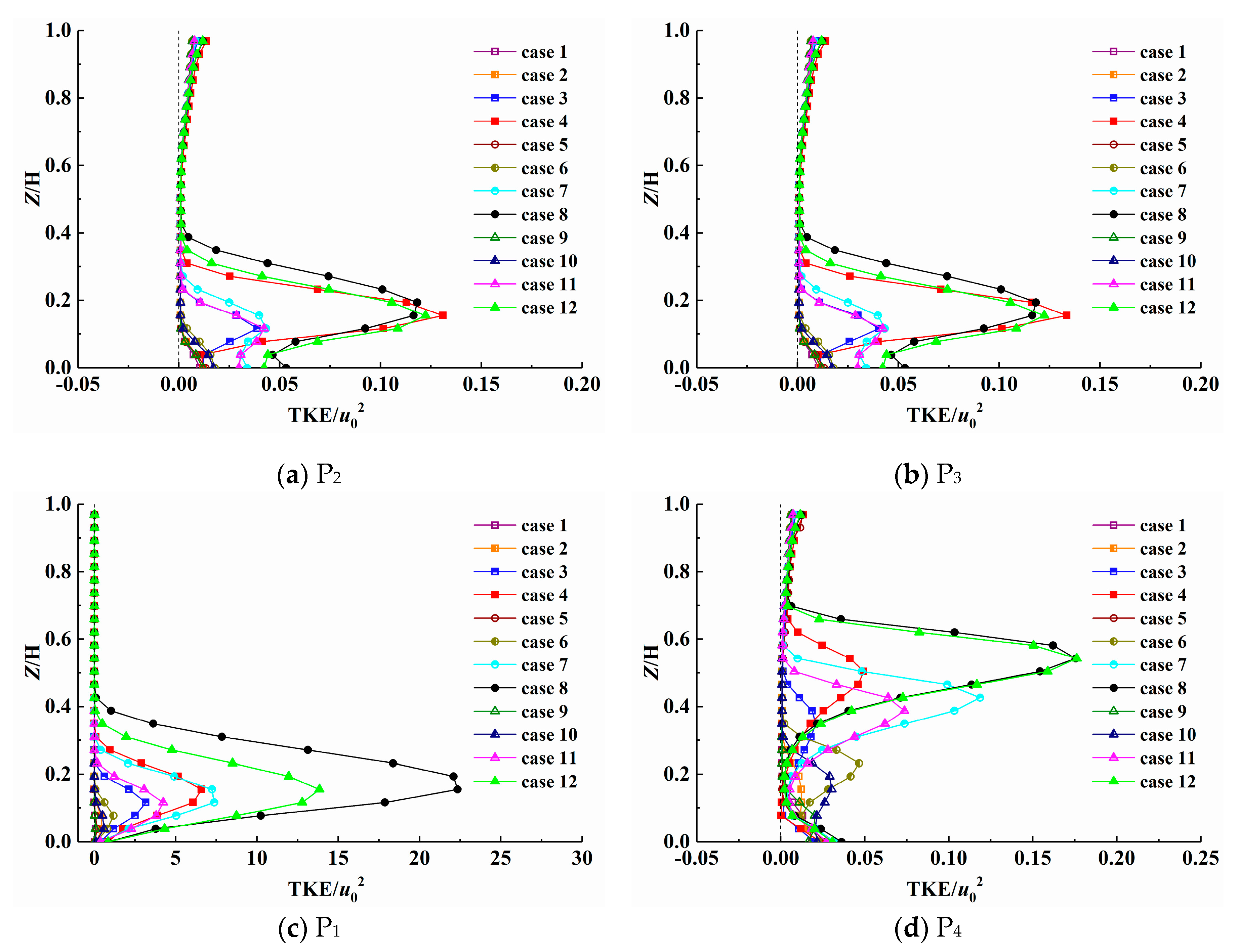
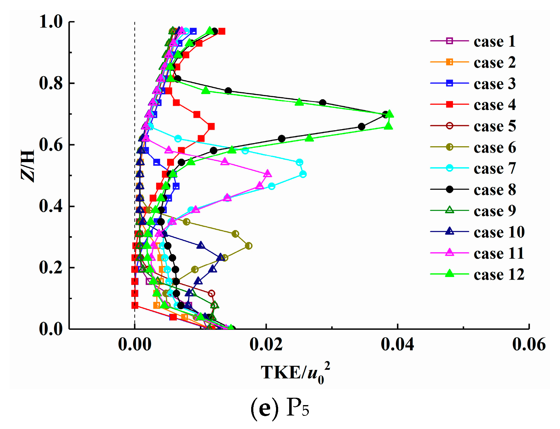
3.2. The Analysis of Turbulent Kinetic Energy (TKE)

When the flow velocity is relatively low, the flow in the straight channel is laminar, and the TKE (calculated by Equation (17)) near the sidewall is relatively large due to the influence of the flow velocity fluctuation. When the jet beam enters the water, the flow fluctuation increases, and the TKE increases as the jet beam passes. In this work, several TKE distributed along the water depth at several locations are selected to analyze the influence of the jet orifice shape and velocity ratio on the distribution of TKE in the channel, as shown in Figure 8. As shown in Figure 1, P₁ is the center of the jet orifice, the distances of P₂ and P₃ to P₁ are both X/D = 4, and the distances of P₄ and P₅ to P₁ are Y/D = 10 and 20, respectively.

$$TKE=\frac{1}{2}[{(u^{\prime })}^2+{(v^{\prime })}^2+{({\omega }^{\prime })}^2]$$

(17)

where $u^{\prime }$, $v^{\prime }$, and ${\omega }^{\prime }$ represent the fluctuating flow velocity in the X, Y, and Z directions, respectively.

It can be seen from Figure 8a,b that the TKE value along the water depth is distributed symmetrically under different cases at symmetrical positions on both sides of the center of the jet orifice. Overall, the maximum TKE value gradually increases as the velocity ratio increases, and the influence of the different jet orifice shapes is not significant. When the flow velocity is small (r = 2 and 5), the maximum TKE values under different cases are relatively close to each other and adjacent to the channel. When the flow velocity is high (r = 10 and 15), the maximum TKE value significantly increases, and the height of the corresponding occurrences also increases significantly. In both situations, the height at which the maximum TKE appears is Z/H = 0.16. As shown in Figure 8c, the variation in the TKE value at the center of the jet orifice along the water depth under different cases has a notable pattern. As the velocity ratio increases, the maximum TKE increases gradually as does the corresponding height of the occurrences. With different jet orifice shapes, the heights where the maximum TKE value occurs under the same velocity ratio are basically the same, but the corresponding numerical values are significantly different: the maximum TKE value of the square jet is the largest, and the maximum TKE value of the round jet is the smallest.

According to Figure 8d, at the position Y/D = 10 away from the jet orifice downstream of the channel, the maximum TKE value gradually increases as the velocity ratio increases, as does the corresponding height of the occurrences. The maximum TKE value of the circular jet occurs at the smallest height and its value is also the smallest. The maximum TKE value of the square jet occurs at the largest height, and its value is also the largest. When the velocity ratio is small (r = 2 and 5), the maximum TKE is close to the channel, and when the velocity ratio is high (r = 10 and 15), the heights at which the maximum TKE values occur for different jet orifice shapes differ greatly. When r = 10, the maximum TKE values corresponding to the circular orifice, square orifice, and rectangular orifice are Z/H = 0.35, 0.49, and 0.43 respectively, and when r = 15, the maximum TKE values are Z/H = 0.50, 0.54, and 0.54, respectively. Combined with the earlier analysis of Figure 7, it is believed that the TKE value is highly related to the spiral deflection of the jet beam. The height at which the spiral deflection occurs is the largest for the square jet, followed by the rectangular jet and then the round jet; thus, the height corresponding to the maximum TKE value also exhibits a similar distribution pattern. According to Figure 8e, the variation in the TKE distribution along the water depth at a distance Y/D = 20 from the jet outlet is relatively complex. Further analysis shows that the variation pattern of the TKE value is the same as that at Y/D = 10, but the maximum TKE value is significantly reduced, and the positions at which the maximum TKE value appears under different cases increase remarkably.

Analysis of Figure 8a–e shows that the abscissa of Figure 8c is significantly larger than that of the other figures. This is because the turbulence is relatively strong at the center of the jet orifice due to the sharp collision between the jet and the original water in the open channel. Then, the TKE gradually decreases as the distance to the jet hole increases. The four points (P₂, P₃, P₄, and P₅) selected in this paper are far from the jet orifice (P₁) and close to the edge of the area affected by the jet. Therefore, the turbulent kinetic energy at these four positions is significantly smaller than that at the position of the jet orifice.

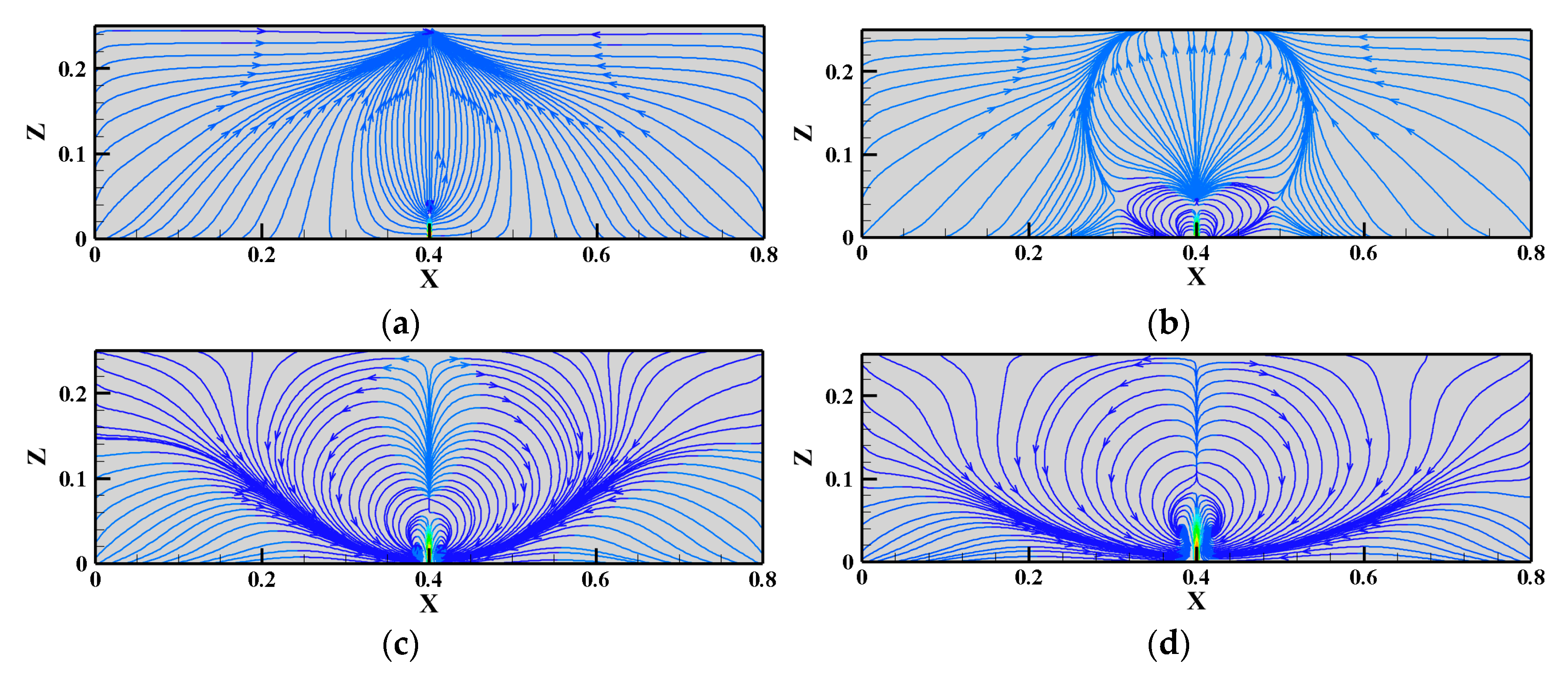
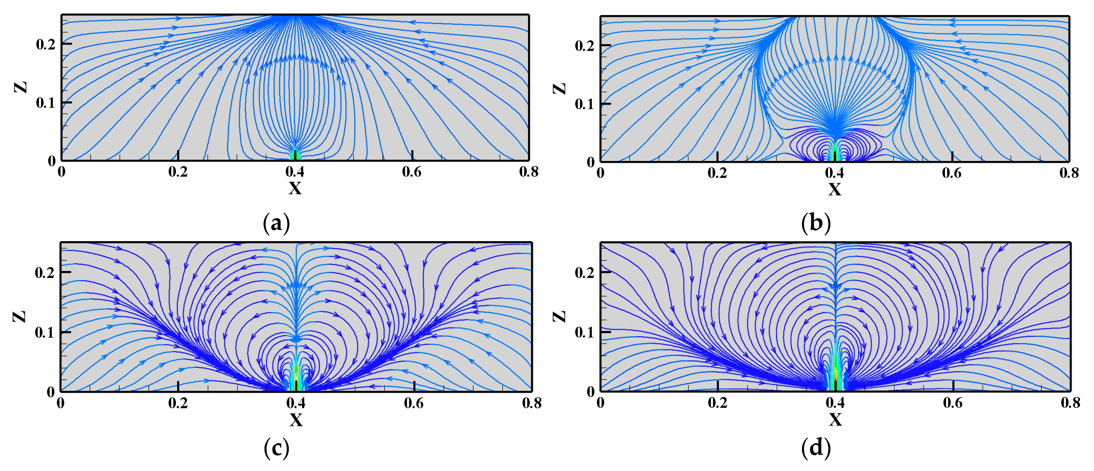
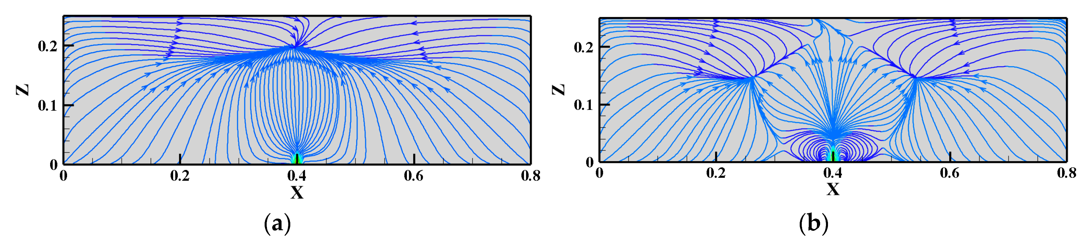
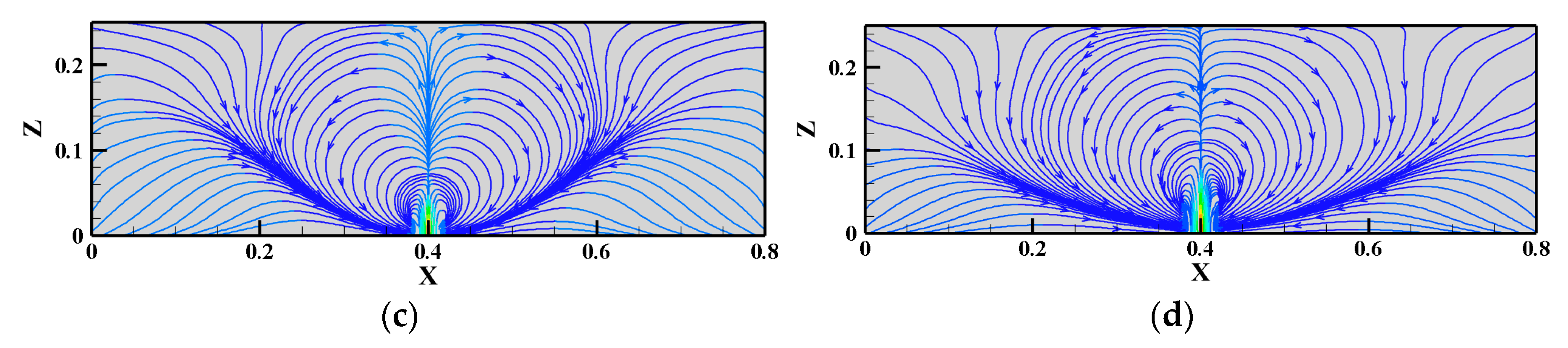
3.3. The Analysis of Vortex

After the jet beam enters the channel, the velocity of the original water changes significantly, and vortices can be found near the jet beam. In this study, the vortex characteristics at the cross-section Y = 0 under different cases are analyzed, as shown in Figure 9, Figure 10 and Figure 11 (where the legend in the cloud plots of the velocity is consistent with that in Figure 7).

Figure 9 shows that there is a very small vortex at the deflection position of the cross-sectional jet orifice when the circular jet has a velocity ratio of 2 because the jet velocity is too small, which causes the jet beam to deflect along the Y direction near the channel while only slightly deflecting in the X direction. When the velocity ratio is 5, there is a notable kidney vortex near the jet orifice, the water above the kidney vortex moves upward, the water on both sides deflects on the upper side of the vortex, and the kidney vortex and the upper streamtrace lines form a circular distribution on the plane. When the velocity ratio is 10, the range of the kidney vortex is further expanded. The region above the jet orifice is within the range of the kidney vortex, and both sides are affected by the kidney vortex, resulting in a notable streamtrace line convergence near the lower side of the kidney vortex. When the velocity ratio is 15, the plane streamtrace line distribution is basically consistent with that when the velocity ratio is 10, with the main difference being the further expanded range of the kidney vortex. An analysis of Figure 10 and Figure 11 shows that as the velocity ratio increases, the range of the kidney vortex increases continuously.

The cross-sectional streamtrace distribution under different orifice shapes and the same velocity ratio as shown in Figure 9, Figure 10 and Figure 11 was analyzed. When the velocity ratio is 2, the shapes of the streamtrace line distribution of the circular and square jet outlets are basically the same, and the height of the converged ellipse-like streamtrace lines above the section of the rectangular jet is reduced significantly. When the velocity ratio is 5, as the shape of the jet orifice gradually changes from circular to rectangular, the kidney vortex and the shapes formed in the upper convergence region gradually develop from circular to pentagonal. It is believed that, with a relatively small velocity ratio, the influence height corresponding to the circular, square, and rectangular jet orifices gradually decrease, while different jet orifice shapes result in different coverages and thus different streamtrace line distributions. When the velocity ratios are 10 and 15, there is no significant difference in the sectional distribution of the kidney vortex with different jet outlet shapes.

4. Conclusions

In this study, the realizable k-ε turbulent model was used to analyze the 3D flow structure, TKE, and vortex structure of water under jets with different orifice shapes and velocity ratios in straight channels. The conclusions are as follows:

(1)

The flow trajectory of the vertical jet in the channel exhibited notable 3D characteristics, and the jet orifice shape and velocity ratio significantly affected the spiral characteristics of the flow. As the velocity ratio increased, the number of spiral deflections of the jet beam increased gradually, and the magnitude became larger. The circular jet beam had the largest height and the smallest vertical height of the spiral deflection, the square jet had the largest vertical height at which the spiral deformation occurs, and the rectangular jet had the smallest jet height.

(2)

As the velocity ratio increased, the maximum TKE value gradually increased, and the height corresponding to the maximum value also gradually increased. The maximum TKE value of the circular jet was the smallest and occurred at the smallest height, the maximum TKE value of the square jet was the largest and occurred at the largest height. As the downstream distance increased, the maximum TKE value gradually decreased, and the height at which the maximum TKE value occurs gradually increased.

(3)

As the velocity ratio increased, the influence range of the kidney vortex increased. When the shape of the jet orifice gradually changed from circular to square and rectangular, the shape formed by the kidney vortex and the region above it gradually changed from circular to pentagonal, indicating that the shape of the jet orifice affects the shape distribution of the cross-sectional vortex.

References

1. Papanicolaou, P.; List, E. Investigation of round vertical turbulent buoyant jets. J. Fluid Mech. 1988, 195, 341–391. [Google Scholar] [CrossRef]
2. Peterson, J.; Bayazitoglu, Y. Measurements of velocity and turbulence in vertical axisymmetric isothermal and buoyant jets. J. Heat Trans. 1992, 114, 135–142. [Google Scholar] [CrossRef]
3. Mossa, M.; De Serio, F. Rethinking the process of detrainment: Jets in obstructed natural flows. Sci. Rep. 2016, 6, 39103. [Google Scholar] [CrossRef] [PubMed] [Green Version]
4. Eroglu, A.; Breidenthal, R.E. Exponentially accelerating jet in crossflow. AIAA J. 1998, 36, 1002–1009. [Google Scholar] [CrossRef]
5. Morton, B.R.; Ibbetson, A. Jets deflected in a crossflow. Exp. Therm. Fluid Sci. 1996, 12, 112–133. [Google Scholar] [CrossRef]
6. Scorer, R.S. Natural Aerodynamics; Pergamon: Oxford, UK, 1958. [Google Scholar]
7. Kelso, R.M.; Lims, T.T.; Perry, A.E. An experimental study of round jets in cross-flow. J. Fluid Mech. 1996, 306, 111–144. [Google Scholar] [CrossRef]
8. Yuan, H.; Xu, W.L.; Li, R.; Feng, Y.Z.; Hao, Y.F. Spatial Distribution Characteristics of Rainfall for Two-Jet Collisions in air. Water 2018, 10, 1600. [Google Scholar] [CrossRef] [Green Version]
9. Gao, M.; Huai, W.X.; Xiao, Y.Z.; Yang, Z.H.; Jin, B. Large eddy simulation of a vertical buoyant jet in a vegetated channel. Int. J. Heat Fluid Flow 2018, 70, 114–124. [Google Scholar] [CrossRef]
10. Chai, X.; Iyer, P.S.; Mahesh, K. Numerical study of high speed jets in crossflow. J. Fluid Mech. 2015, 785, 152–188. [Google Scholar] [CrossRef] [Green Version]
11. Guan, H.; Wu, C. Large-eddy simulations and vortex structures of turbulent jets in crossflow. Sci. China Phys. Mech. 2007, 50, 118–132. [Google Scholar] [CrossRef]
12. Smith, S.H.; Mungal, M.G. Mixing, structure and scaling of the jet in crossflow. J. Fluid Mech. 1998, 357, 83–122. [Google Scholar] [CrossRef]
13. Wang, H.W.; Law, A.W.K. Second-order integral model for a round turbulent buoyant jet. J. Fluid Mech. 2002, 459, 397–428. [Google Scholar] [CrossRef]
14. Huai, W.X.; Li, W.; Peng, W.Q. Calculation and behavior analysis on turbulent jets in cross-flow. J. Hydrau. Eng. 1998, 4, 7–14. (In Chinese) [Google Scholar]
15. Andreopolous, J.; Rodi, W. Experimental investigation of jets in a cross-flow. J. Fluid Mech. 1984, 138, 43–127. [Google Scholar]
16. Zhu, J.; Shih, T.H. Computation of confined crossflow jets with three turbulence models. Int. J. Numer. Methods Fluids 1994, 19, 939–956. [Google Scholar] [CrossRef] [Green Version]
17. Zeng, Y.H.; Huai, W.X. Characteristics of round thermal discharging in a flowing environment. J. Hydro-Environ. Res. 2009, 2, 164–171. [Google Scholar] [CrossRef]
18. Ma, F.; Satish, M.; Islam, M.R. Large eddy simulation of thermal jets in cross flow. Eng. Appl. Comput. Fluid Mech. 2007, 1, 25–35. [Google Scholar] [CrossRef] [Green Version]
19. Rogowski, K.; Hansen, M.O.L.; Maroński, R.; Lichota, P. Scale Adaptive Simulation Model for the Darrieus Wind Turbine. J. Phys. Conf. Ser. 2016, 753, 022050. [Google Scholar] [CrossRef]
20. Haven, B.A.; Kurosaka, M. Kidney and anti-kidney vortices in crossflow jets. J. Fluid Mech. 1997, 352, 27–64. [Google Scholar] [CrossRef]
21. Shih, T.H.; Liou, W.W.; Shabbir, A.; Yang, Z.; Zhu, J. A new k-ε eddy viscosity model for high reynolds number turbulent flows. Comput. Fluids 1995, 24, 227–238. [Google Scholar] [CrossRef]
22. Hirt, C.W.; Nichols, B.D. Volume of fluid (VOF) method for the dynamics of free boundaries. J. Comput. Phys. 1981, 39, 201–225. [Google Scholar] [CrossRef]
23. Patankar, S.V.; Spalding, D.B. A calculation procedure for heat, mass and momentum transfer in three-dimensional parabolic flows. Int. J. Hear Mass Transf. 1972, 15, 1787–1806. [Google Scholar] [CrossRef]
24. Malcangio, D.; Mossa, M. A laboratory investigation into the influence of a rigid vegetation on the evolution of a round turbulent jet discharged within a cross flow. J. Environ. Manag. 2016, 173, 105–120. [Google Scholar] [CrossRef] [PubMed]
25. Celik, I.B.; Ghia, U.; Roache, P.J.; Freitas, C.J. Procedure of estimation and reporting of uncertainty due to discretization in CFD applications. J. Fluids Eng. 2008, 130, 078001. [Google Scholar]
Figure 1. Three-dimensional (3D) view of the model layout.
Energies 13 01505 g001
Figure 2. The grid of the numerical model.
Energies 13 01505 g002
Figure 3. Mass flow rate error (MFRE) time-history curve.
Energies 13 01505 g003
Figure 4. Vertical distribution of the grid convergence index (GCI) in jet orifice centerline.
Energies 13 01505 g004
Figure 5. Distribution of the vertical flow velocity along the water depth at different locations.
Energies 13 01505 g005
Figure 6. 3D structure of the jet streamtrace.
Energies 13 01505 g006
Figure 7. Variations of streamtraces under different cases: (a) case 1, (b) case 5, (c) case 9, (d) case 2, (e) case 6, (f) case 10, (g) case 3, (h) case 7, (i) case 11, (j) case 4, (k) case 8, (l) case 12.
Energies 13 01505 g007aEnergies 13 01505 g007b
Figure 8. Distribution of the turbulent kinetic energy (TKE) values at different locations along the water depth: (a) P2, (b) P3, (c) P1, (d) P4, (e) P5.
Energies 13 01505 g008aEnergies 13 01505 g008b
Figure 9. Vortex of the circular jet at cross-section Y = 0: (a) case 1, (b) case 2, (c) case 3, (d) case 4.
Energies 13 01505 g009
Figure 10. Vortex of the square jet at cross-section Y = 0: (a) case 5, (b) case 6, (c) case 7, (d) case 8.
Energies 13 01505 g010
Figure 11. Vortex of the rectangular jet at cross-section Y = 0: (a) case 9, (b) case 10, (c) case 11, (d) case 12.
Energies 13 01505 g011aEnergies 13 01505 g011b