Planning Annual LNG Deliveries with Transshipment


Abstract
:1. Introduction
2. Literature Review
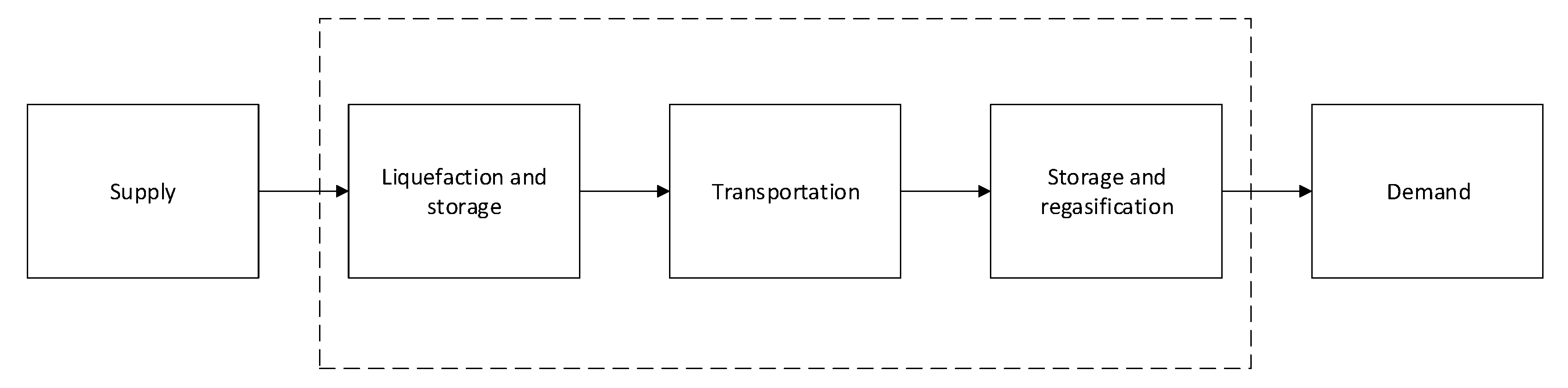
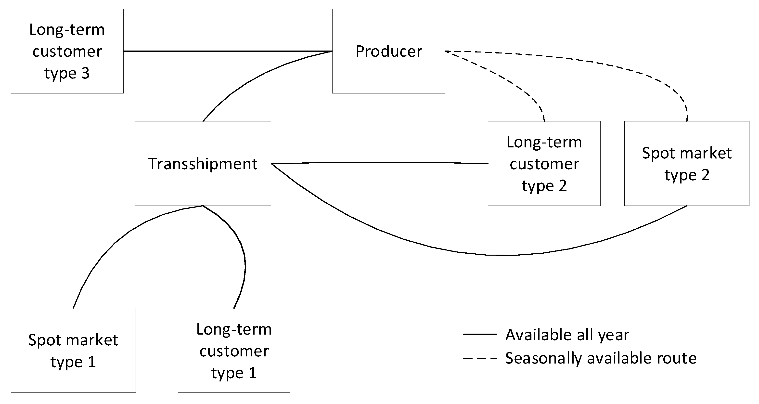
3. Problem Description
4. Model Formulation
4.1. Notation
| Sets | |
| Set of delivery periods to customers | |
| K | Set of departure periods determining sailing speed of the LNG carriers |
| Set of departure periods when the direct route to some customers is closed, . | |
| P | Set of ports. |
| Set of unloading ports that can be visited by carrier v. | |
| Set of ports that can be visited from the production port, . | |
| Set of ports that can be visited from the transshipment port, . | |
| Set of customer ports, . | |
| Set of ports that can be visited both directly and via transshipment, . | |
| Set of long-term customers, . | |
| Set of production ports, . | |
| Set of spot markets, . | |
| Set of transshipment ports, . | |
| Set of possible nodes which indicates the m-th port call at port i. | |
| V | Set of LNG carriers. |
| Set of LNG carriers of type A, . These carriers only load at the production port. | |
| Set of LNG carriers of type B, . These carriers only load at the transshipment port. | |
| Indices | |
| g | Periods index for delivery, . |
| Port index, . | |
| k | Period index for departure time, . |
| Port call index. | |
| v | Carrier index, . |
| Parameters | |
| Boil-off for a round trip from port i to port j with carrier v. | |
| Cost of a round trip from port i to port j with carrier v. | |
| Demand (in m) at customer j in delivery period g, . | |
| Loading capacity for carriers of type v, . | |
| Initial position of carrier v, . | |
| Production rate at port i, . | |
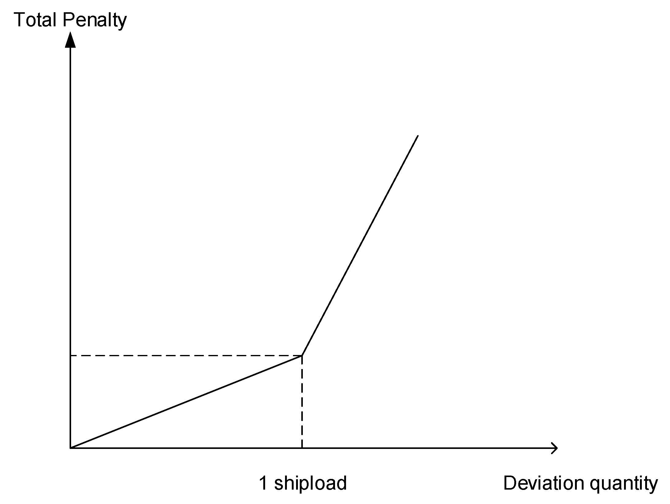
| Penalty per m for annual over-delivery at customer j exceeding one shipload, . | |
| Penalty per m for annual over-delivery at customer j below one shipload, . | |
| Penalty per m for over-delivery in delivery period g at customer j, . | |
| Revenue from selling one shipload LNG on carrier v to spot market j. | |
| Initial storage at port i, . | |
| Upper bound on inventory level at port i. | |
| Lower bound on inventory level at port i. | |
| End of planning horizon. | |
| End of year, . | |
| Start of delivery period g, . | |
| Start of departure period k, . | |
| Minimum operational time required by port i between two consecutive visits. | |
| Sailing time of carrier v for traveling from port i to j when starting in departure period k. | |
| Penalty per m for annual under-delivery at customer j exceeding one-shipload, . | |
| Penalty per m for annual under-delivery at customer j below one-shipload, . | |
| Penalty per m for under-delivery in delivery period g at customer j, . | |
| Sufficiently small number. | |
| Maximum number of port calls at port i, . | |
| Decision variables | |
| Over-delivery (in m) at customer j exceeding one shipload over the entire planning horizon, | |
| . | |
| Over-delivery (in m) at customer j below one shipload over the entire planning horizon, . | |
| Over-delivery (in m) at customer j in delivery period g, . | |
| Inventory level at port i at the beginning of the port call, . | |
| Start of voyage from node , . | |
| Under-delivery (in m) at customer j exceeding one shipload over the entire planning horizon, | |
| . | |
| Under-delivery (in m) at customer j below one shipload over the entire planning horizon, . | |
| Under-delivery (in m) at customer j in delivery period g, . | |
| 1 if node is visited by carrier v, 0 otherwise, . | |
| 1 if node is visited by any carrier, 0 otherwise, . | |
| 1 if carrier v starts the voyage from unloading node back to loading node in delivery | |
| period g, 0 otherwise, . | |
| 1 if a round trip of carrier v from loading node to unloading node starts in departure | |
| period k, 0 otherwise, . | |
| 1 if start of voyage from node is greater or equal to the start time of departure period , | |
| 0 otherwise, . | |
| 1 if start of voyage from node is greater or equal to the start time of delivery period , | |
| 0 otherwise, . | |
4.2. Model Formulation
4.2.1. Objective Function
4.2.2. Routing and Symmetry Breaking Constraints
4.2.3. Constraints for Grouping Departures and Contracted Deliveries
4.2.4. Sailing Time Constraints
4.2.5. Inventory Constraints
4.2.6. Contract Management and Non-Negativity Constraints
5. Solution Method
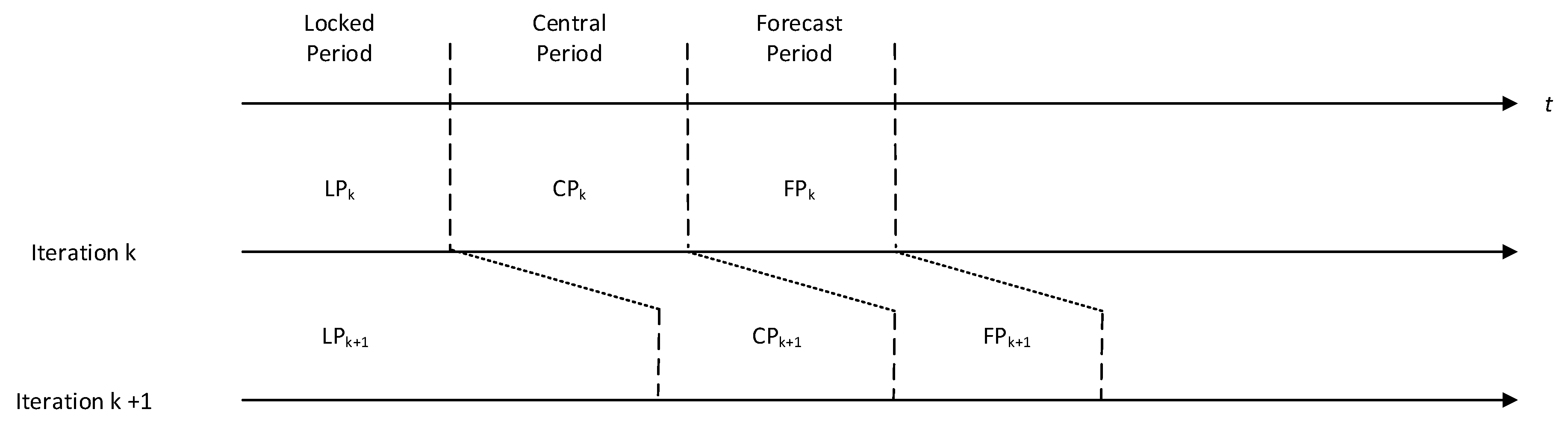
5.1. The Rolling Horizon Framework
5.2. RHH for Continuous Time Formulations
6. Computational Study
6.1. Input Data
6.1.1. Port Information
6.1.2. Carrier Information
6.1.3. Deviation Penalties
6.1.4. Planning Horizon and Initial Values
6.2. Case Study
6.2.1. Overview of the Cases
6.2.2. Computational Results
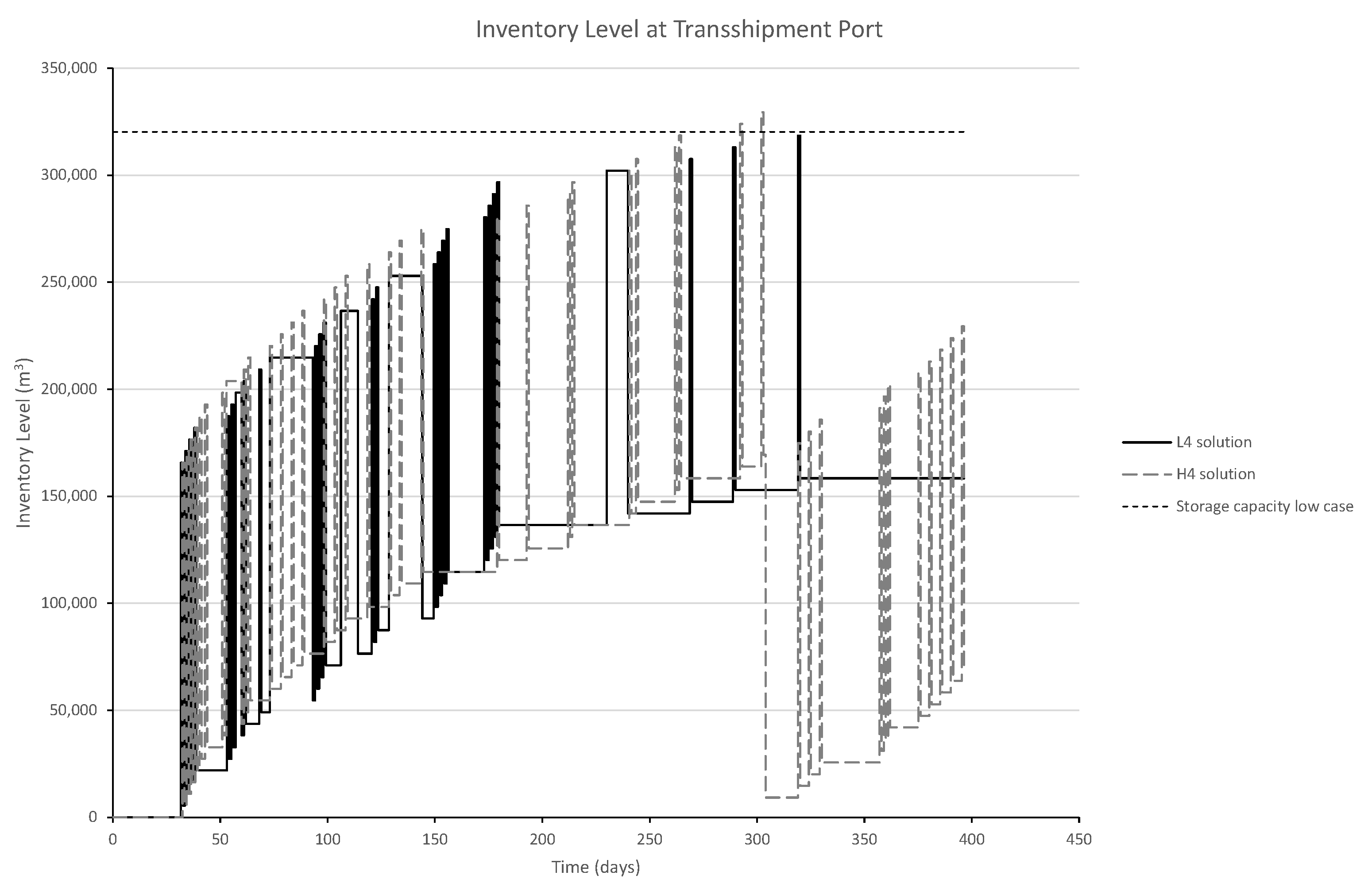
6.2.3. Differences in Solution Structure
7. Conclusions
Author Contributions
Funding
Conflicts of Interest
References
- IEA. World Energy Outlook 2019; OECD Publishing: Paris, France, 2019. [Google Scholar]
- GIIGNL. The LNG Industry GIIGNL Annual Report 2019; The International Group of Liquefied Natural Gas Importers: Neuilly-sur-Seine, France, 2019. [Google Scholar]
- Yamal LNG Eclipses Annual Nameplate Production. Available online: https://www.lngworldnews.com/yamal-lng-eclipses-annual-nameplate-production/ (accessed on 8 March 2020).
- Arctic LNG 2 Project. Available online: http://www.novatek.ru/en/business/arctic-lng/ (accessed on 8 March 2020).
- Andersson, H.; Christiansen, M.; Desaulniers, G.; Rakke, J.G. Creating annual delivery programs of liquefied natural gas. Optim. Eng. 2017, 18, 299–316. [Google Scholar] [CrossRef]
- Rakke, J.G.; Stålhane, M.; Moe, C.R.; Christiansen, M.; Andersson, H.; Fagerholt, K.; Norstad, I. A rolling horizon heuristic for creating a liquefied natural gas annual delivery program. Transp. Res. Part Emerg. Technol. 2011, 19, 896–911. [Google Scholar] [CrossRef]
- Stålhane, M.; Rakke, J.G.; Moe, C.R.; Andersson, H.; Christiansen, M.; Fagerholt, K. A construction and improvement heuristic for a liquefied natural gas inventory routing problem. Comput. Ind. Eng. 2012, 62, 245–255. [Google Scholar] [CrossRef]
- Papageorgiou, D.J.; Nemhauser, G.L.; Sokol, J.; Cheon, M.S.; Keha, A.B. MIRPLib—A library of maritime inventory routing problem instances: Survey, core model, and benchmark results. Eur. J. Oper. Res. 2014, 235, 350–366. [Google Scholar] [CrossRef]
- Christiansen, M.; Fagerholt, K. Ship routing and scheduling in industrial and tramp shipping. In Vehicle Routing: Problems, Methods, and Applications, 2nd ed.; Toth, P., Vigo, D., Eds.; SIAM—Society for Industrial and Applied Mathematics: Philadelphia, PA, USA, 2014; pp. 381–408. [Google Scholar]
- Christiansen, M.; Fagerholt, K.; Nygreen, B.; Ronen, D. Ship routing and scheduling in the new millennium. Eur. J. Oper. Res. 2013, 228, 467–483. [Google Scholar] [CrossRef]
- Halvorsen-Weare, E.E.; Fagerholt, K. Routing and scheduling in a liquefied natural gas shipping problem with inventory and berth constraints. Ann. Oper. Res. 2013, 203, 167–186. [Google Scholar] [CrossRef] [Green Version]
- Al-Haidous, S.; Msakni, M.K.; Haouari, M. Optimal planning of liquefied natural gas deliveries. Transp. Res. Part Emerg. Technol. 2016, 69, 79–90. [Google Scholar] [CrossRef]
- Mutlu, F.; Msakni, M.K.; Yildiz, H.; Sönmez, E.; Pokharel, S. A comprehensive annual delivery program for upstream liquefied natural gas supply chain. Eur. J. Oper. Res. 2016, 250, 120–130. [Google Scholar] [CrossRef]
- Grønhaug, R.; Christiansen, M. Supply chain optimization for the liquefied natural gas business. In Innovations in Distribution Logistics; Bertazzi, L., Speranza, M.G., van Nunen, J., Eds.; Springer: Berlin, Germany, 2009; pp. 195–218. [Google Scholar]
- Uggen, K.T.; Fodstad, M.; Nørstebø, V.S. Using and extending fix-and-relax to solve maritime inventory routing problems. TOP 2013, 21, 355–377. [Google Scholar] [CrossRef]
- Goel, V.; Furman, K.C.; Song, J.H.; El-Bakry, A.S. Large neighborhood search for LNG inventory routing. J. Heuristics 2012, 18, 821–848. [Google Scholar] [CrossRef]
- Song, J.H.; Furman, K.C. A maritime inventory routing problem: Practical approach. Comput. Oper. Res. 2013, 40, 657–665. [Google Scholar] [CrossRef]
- Shao, Y.; Furman, K.C.; Goel, V.; Hoda, S. A hybrid heuristic strategy for liquefied natural gas inventory routing. Transp. Res. Part C Emerg. Technol. 2015, 53, 151–171. [Google Scholar] [CrossRef]
- Christiansen, M. Decomposition of a combined inventory and time constrained ship routing problem. Transp. Sci. 1999, 33, 3–16. [Google Scholar] [CrossRef]
- Al-Khayyal, F.; Hwang, S.J. Inventory constrained maritime routing and scheduling for multi-commodity liquid bulk, Part I: Applications and model. Eur. J. Oper. Res. 2007, 176, 106–130. [Google Scholar] [CrossRef]
- Agra, A.; Christiansen, M.; Delgado, A. Discrete time and continuous time formulations for a short sea inventory routing problem. Optim. Eng. 2017, 18, 269–297. [Google Scholar] [CrossRef] [Green Version]
- Papageorgiou, D.J.; Cheon, M.S.; Harwood, S.; Trespalacios, F.; Nemhauser, G.L. Recent progress using matheuristics for strategic maritime inventory routing. In Modeling, Computing and Data Handling Methodologies for Maritime Transportation; Konstantopoulos, C., Pantziou, G., Eds.; Springer: Cham, Switzerland, 2018; pp. 59–94. [Google Scholar]
- Savelsbergh, M.; Song, J.H. Inventory routing with continuous moves. Comput. Oper. Res. 2007, 34, 1744–1763. [Google Scholar] [CrossRef]
- Agra, A.; Christiansen, M.; Delgado, A.; Simonetti, L. Hybrid heuristics for a short sea inventory routing problem. Eur. J. Oper. Res. 2014, 236, 924–935. [Google Scholar] [CrossRef]
- Mercé, C.; Fontan, G. MIP-based heuristics for capacitated lotsizing problems. Int. J. Prod. Econ. 2003, 85, 97–111. [Google Scholar] [CrossRef]
- Marine Traffic Voyage Planner. Available online: https://www.marinetraffic.com/en/ais/home/centerx:141.1/centery:60.2/zoom:7 (accessed on 15 February 2020).
- IGU. 2019 World LNG Report; International Gas Union: Barcelona, Spain, 2019. [Google Scholar]
- World Bank Group. Commodity Markets Outlook, October 2019; World Bank: Washington, DC, USA, 2019. [Google Scholar]
- Design an LNG Ice-Breaker Ship. Available online: https://www.ep.total.com/en/areas/liquefied-natural-gas/our-yamal-lng-project-russia/lng-ice-breaker-first-liquefied-natural-gas (accessed on 15 February 2020).
- Card, J.; Lee, H. Leading technology for next generation of LNG carriers. In Proceedings of the Fifteenth International Offshore and Polar Engineering Conference, Seoul, Korea, 19–24 June 2005; International Society of Offshore and Polar Engineers: Mountain View, CA, USA, 2005. ISOPE-I-05-013. [Google Scholar]
- Lopac, A.A. Recent trends in transporting of LNG, liquefied natural gas. In Proceedings of the ICTS2008-Transport Policy, Portoroz, Slovenia, 28–29 May 2008. [Google Scholar]
- Tolls Calculator. Available online: https://www.suezcanal.gov.eg/English/Tolls/Pages/TollsCalculator.aspx (accessed on 7 June 2018).
- Hasan, M.F.; Zheng, A.M.; Karimi, I. Minimizing boil-off losses in liquefied natural gas transportation. Ind. Eng. Chem. Res. 2009, 48, 9571–9580. [Google Scholar] [CrossRef]
- The Difference with LNG? It’s Just about Boil-off Isn’t It? Available online: https://www.reedsmith.com/en/perspectives/2014/06/the-difference-with-lng–its-just-about-boiloff-is (accessed on 15 February 2020).
- Yamal LNG Transshipment Tank at Zeebrugge Springs into Action. Available online: https://www.lngworldnews.com/yamal-lng-transshipment-tank-at-zeebrugge-springs-into-action/ (accessed on 8 March 2020).
- First Simultaneous Transhipment of Yamal LNG. Available online: https://portofzeebrugge.be/en/news-events/first-simultaneous-transhipment-yamal-lng (accessed on 15 February 2020).
- MOL, JBIC, and NOVATEK Sign Cooperation Agreement for LNG Transshipment Projects in Kamchatka and Murmansk. Available online: https://www.mol.co.jp/en/pr/2019/19063.html (accessed on 15 February 2020).

| Port Number | Type | Direct Route | via Transshipment | Direct Route Distance (nm) | Distance from Transshipment (nm) |
|---|---|---|---|---|---|
| 1 | Production | - | - | - | - |
| 2 | Long-term | Seasonal | Yes | 5959.7 | 11,067.2 |
| 3 | Long-term | Seasonal | Yes | 6054 | 11,160.6 |
| 4 | Spot | Seasonal | Yes | 5348.9 | 11,058.2 |
| 5 | Long-term | Seasonal | Yes | 10,268.2 | 10,955.9 |
| 6 | Long-term | Seasonal | Yes | 6010.9 | 10,862.2 |
| 7 | Long-term | Yes | No | 2784.9 | - |
| 8 | Long-term | No | Yes | - | 2080.2 |
| 9 | Spot | No | Yes | - | 741.7 |
| 10 | Transshipment | Yes | - | 2661.8 | - |
| Instance | Storage Capacity at Transshipment | Planning Horizon for RHH (months) |
|---|---|---|
| HF | High | 13+1 |
| H2 | High | 1+1 |
| H3 | High | 2+1 |
| H4 | High | 3+1 |
| LF | Low | 13+1 |
| L2 | Low | 1+1 |
| L3 | Low | 2+1 |
| L4 | Low | 3+1 |
| Instance | Best Solution | Best Bound Last Iteration | Gap Last Iteration | Not Optimal/Total Iterations | Total Run Time (h) |
|---|---|---|---|---|---|
| HF | Not solved | - | - | - | >24 |
| H2 | 542,340,683 | 460,334,852 | 15.12% | 1/12 | 4.5 |
| H3 | 224,109,041 | 224,091,574 | 0% | 0/7 | 1.3 |
| H4 | 217,427,397 | 202,055,902 | 7.07% | 2/5 | 11.4 |
| LF | Not solved | - | - | - | >24 |
| L2 | Infeasible | - | - | - | - |
| L3 | Infeasible | - | - | - | - |
| L4 | 1,075,488,728 | 1,075,402,397 | 0% | 1/5 | 5.1 |
| Instance | Port 1 | Port 2 | Port 3 | Port 4 | Port 5 | Port 6 | Port 7 | Port 8 | Port 9 | Port 10 |
|---|---|---|---|---|---|---|---|---|---|---|
| H4 | 79 | 6 | 5 | 7 | 18 | 5 | 17 | 19 | 3 | 43 |
| L4 | 76 | 6 | 5 | 5 | 19 | 6 | 19 | 15 | 1 | 29 |
© 2020 by the authors. Licensee MDPI, Basel, Switzerland. This article is an open access article distributed under the terms and conditions of the Creative Commons Attribution (CC BY) license (http://creativecommons.org/licenses/by/4.0/).
Share and Cite
Li, M.; Schütz, P. Planning Annual LNG Deliveries with Transshipment. Energies 2020, 13, 1490. https://doi.org/10.3390/en13061490
Li M, Schütz P. Planning Annual LNG Deliveries with Transshipment. Energies. 2020; 13(6):1490. https://doi.org/10.3390/en13061490
Chicago/Turabian StyleLi, Mingyu, and Peter Schütz. 2020. "Planning Annual LNG Deliveries with Transshipment" Energies 13, no. 6: 1490. https://doi.org/10.3390/en13061490
APA StyleLi, M., & Schütz, P. (2020). Planning Annual LNG Deliveries with Transshipment. Energies, 13(6), 1490. https://doi.org/10.3390/en13061490