Analysis and Application of the Direct Flux Control Sensorless Technique to Low-Power PMSMs

Abstract

In the field of sensorless control of permanent magnet synchronous motors (PMSMs), different techniques based on machine anisotropies have been studied and implemented successfully. Nevertheless, most proposed approaches extract the rotor position information from the measured machine currents, that, when applied to low-power machines, might require high-bandwidth current sensors. An interesting alternative is given by sensorless techniques that exploit the star-point voltage of PMSMs, such as the direct flux control technique. This work aims at analyzing the conditions of applicability of such technique by considering a more thorough description of the machine inductance matrix. After a comprehensive mathematical description of the technique and characterization of the machine anisotropy information that is extracted from the star-point voltage, simulation as well as experimental results conducted on a test machine are presented and discussed in order to validate the proposed theory.

1. Introduction

In the last decades, the demand for compact electrical machines and drives able to guarantee high performance has been pushing towards the adoption of brushless synchronous motors (SMs) in several application fields ranging from e-mobility to renewable energy production. In particular, permanent magnet synchronous machines (PMSMs) are considered a good alternative to switched reluctance or induction machines because they allow high torque densities as well as enhanced dynamic performance [1].

PMSMs are usually operated under space vector control, therefore, a high resolution position information is required to guarantee the control system performance [2]. Typically, the position information is provided by encoders or resolvers, which increase costs and system complexity and worsen the overall reliability. In order to overcome these issues, several authors have been investigating control techniques able to avoid the mechanical position sensors by exploiting different physical effects in order to estimate the rotor position. Sensorless techniques reported in the literature can be divided into two groups, according to the physical effect on which they rely: induced back-EMF (electro motive force) or machine magnetic anisotropy.

In the first case, since the rotor speed is proportional to the back-EMF amplitude, once the phase voltages and currents are measured, an estimation of the angular position can be obtained by applying model reference adaptive system techniques or state observers. The main limitation of back-EMF based sensorless techniques is their inapplicability at low speeds and/or standstill conditions. In the second case, the rotor position can be estimated by exploiting its relation to the phase inductances due to the machine magnetic anisotropy.

The first technique based on the machine anisotropies, referred to as INFORM, is proposed in [3] and [4], where the motor reactances are obtained by injecting test pulse voltages through modified PWM (Pulse Width Modulation) driving signals and measuring the current signals that are dependent on the rotor position. A different approach is reported in [5], where sensorless operations are based on the injection of a rotating carrier, which induces currents whose amplitude is modulated by the rotor position. In this case, the extraction of the position information relies on the demodulation and the state observation of these signals. In order to avoid the demodulation stage and reduce the computational efforts, the injection of an alternating current in the estimated rotor reference frame is suggested in [6], where a pulsating voltage vector along the q-axis of the estimated rotor reference frame is considered. In this case, an observer is required to extract the position information. Due to the better performance in terms of precision and robustness ensured by alternating current injection methods over the rotating current ones, the former have been deeply investigated in the last decades [7], focusing on alternating carrier or other arbitrary injection schemes [8,9,10,11].

All the aforementioned techniques extract the rotor position information from current measurements. Nevertheless, sensorless operation can be performed by also relying on voltage measurements. Indeed, when current information is not needed for performing torque control or condition monitoring, the cost of the drive system decreases because of the removal of current sensors. This is particularly relevant in embedded drive systems applications, where miniaturization of electronics is a priority. Different works have shown the possibility of using the voltage at the machine star-point in order to perform sensorless operation and several techniques have been applied on different kind of motors. In [12], the zero-sequence voltage is used for sensorless control of induction motors. In [13], the same authors suggest a technique for performing sensorless operation on machines that do not have an accessible star-point. Other sensorless techniques exploiting the zero-sequence voltage for induction motors have been proposed in [14], where a filter has been tuned for distinguishing between the rotor bar and the magnetic saturation effects, in [15], where a technique to reduce noise given by cables has been also proposed and in [16], where the author summarizes and compares several sensorless techniques for induction motors, included a zero-sequence voltage based one. These techniques have been successfully applied also to synchronous machines. In [17], a zero-sequence voltage based approach has been used for the rotor position estimation in PMSMs as an extension to the work [12]. A different technique exploiting the star-point voltage of synchronous machines was proposed in [18] and, later on, was presented under different terminologies such as VirtuHall, direct flux control (DFC) and direct flux observer (DFO). In [19] and in [20], a method to excite the machine for the DFC technique in order to obtain signals that can be used for the estimation of the rotor position has been proposed. In order to improve the quality of such measurements, a Fast resettable integrator circuit (FRIC) was presented in [21,22,23]. Another interesting usage of the zero-sequence voltage for sensorless operation of PMSMs is reported, firstly, in [24], where the machine is operated by exciting two machine phases and by measuring the induced voltage caused by magnetic saturation (IVMS) allowing for the estimation of the rotor position. This technique presented the limitation of allowing only block-commutation so, in order to overcome this limitation, this technique was further developed and proposed in [25]. This technique is capable of operating with magnetically saturated machines and resembles the DFC technique, however the PWM pulse shifting pattern differs. Also, both approaches rely on measurement electronics that can be tuned accordingly to the machine properties, allowing, by adjusting the measurement gain, the machine to operate successfully with machines that exhibit very little variation with respect to the rotor position. Also, in [26], the neutral-point voltage has been modeled in order to allow for a prediction of its fluctuation. The modeling was performed by taking into account the classical PMSM electrical equations and an asymmetric inductance matrix, showing a dependency between self and mutual inductances in the neutral-point voltage. Finally, in order to enhance the accuracy and the robustness of the sensorless control of PMSM drives, two novel techniques based on the utilization of the neutral-point voltage are proposed in [27,28]. The first work deals with a pulsating carrier signal injection while the latter utilizes a square-wave signal injection. Both methods rely on an estimated reference frame that rotates counterclockwise with twice the estimated rotor electrical angular speed. Thus, they allow a simpler demodulation strategy compared to conventional injection-based techniques.

The techniques presented up to this point divide between high-frequency injection methods and zero-sequence voltage based techniques. In the first case, the electrical rotor position is estimated by measuring the current response in the $\alpha$- and $\beta$-axis given a certain excitation. In the second case, instead, the estimation is performed by measuring the change of the zero-sequence voltage with respect to the rotor position. An interesting and thorough comparison between these two technique categories is given in [29]. In this work, a brief example is also presented in order to address this difference. Therefore, because the source of information differs between these techniques, it is important to analyze which synchronous machines can operate with high-frequency injection methods and which ones can operate with zero-sequence voltage based techniques and give applicability conditions for the latter case.

By considering the mathematical description of the star-point voltage dynamic behavior presented in [23], this work aims at presenting and discussing the applicability of star-point voltage exploiting sensorless techniques to the case of PMSMs. In particular, with reference to the DFC technique, given a mathematical description of a PMSM inductance matrix, similar to that of [26], this work aims at modeling the information that can be extracted from the machine star-point voltage with a particular focus on determining the conditions of the machine phase inductances under which no information can be extracted from the zero-sequence voltage. It has to be remarked that the zero-sequence voltage can be expressed as the virtual star-point voltage minus the machine star-point voltage. Thus, the zero-sequence voltage and the star-point voltage are strictly related to each other. This work aims at mathematically characterizing the position error that is expected when the DFC technique is applied and how the error relates to the phase inductances. The rest of this paper is organized into two main sections related to theory and experimental validation, respectively. In Section 2, the theoretical framework for the mathematical description of the star-point voltage dynamic is recalled. Afterwards, the first condition of applicability of star-point voltage exploiting techniques to SMs is introduced and then particularized to PMSMs exhibiting rotor anisotropy and characterized by inductances, which vary with the rotor position. Then, other applicability conditions are presented. Moreover, a thorough analysis is performed by means of simulations in order to relate the reconstructed position error to the machine inductances. Section 3 reports the results of the experimental investigations conducted on a dedicated test PMSM. In order to validate the proposed mathematical derivation, the PMSM has been coupled to a rotation stage unit to allow a precise measurement of the DFC signals over a full electrical period. The sensorless information has been extracted and compared to the high-precision sensor available in the rotation stage unit. Afterwards, the DFC signals have been measured and identified according to the proposed mathematical model. Then, the proposed position error formula has been validated by comparing the measured rotor position with the expected position from the identified DFC signals. Moreover, the PMSM has also been controlled in an acceleration test both under no load and load conditions, in order to evaluate the performance of the proposed technique under dynamic operation. Finally, in the last part of the paper, the main findings are discussed and possible future works are pointed out.

2. Theory

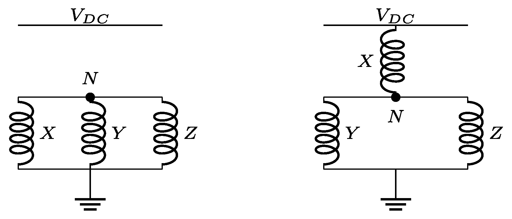
2.1. Analysis of the Star Point Voltage Dynamics in Synchronous Machines

The mathematical description of the star-point voltage dynamics in synchronous machines has been presented extensively in [23]. In this work, after a brief recall of that mathematical framework, the theory is enhanced first by proposing a condition on the applicability of star-point voltage exploiting techniques to SMs and then with considerations concerning the structure of the machine inductance matrix ${\mathbf{L}}_{abc}$. Let us consider the electrical equation of an SM in the phase reference frame where the speed is considered zero. This hypothesis does not limit the validity of this presentation as shown in [23].

$${\mathbf{v}}_{abc}(t)=\mathbf{R}{\mathbf{i}}_{abc}(t)+{\mathbf{L}}_{abc}\frac{d{\mathbf{i}}_{abc}(t)}{dt}$$

(1)

In this work $\mathbf{R}$ is the phase resistance matrix, which is assumed to be diagonal, ${\mathbf{v}}_{abc}(t)={\left[\begin{array}{ccc}{v}_{AN}(t)& v_{BN}(t)& v_{CN}(t)\end{array}\right]}^T$ and ${\mathbf{i}}_{abc}(t)={\left[\begin{array}{ccc}{i}_A(t)& i_B(t)& i_C(t)\end{array}\right]}^T$ are the phase voltage and current vectors and ${\mathbf{L}}_{abc}$ is the inductance matrix defined as:

$${\mathbf{L}}_{abc}=\left[\begin{array}{ccc}{L}_{aa}& L_{ab}& L_{ac}\\ L_{ba}& L_{bb}& L_{bc}\\ L_{ca}& L_{cb}& L_{cc}\end{array}\right].$$

(2)

The matrix ${\mathbf{L}}_{abc}$ is assumed to be a function of the electrical rotor position $\theta$ and invertible per each value of $\theta$. Also, this matrix is a function of the machine current because of the magnetic saturation effect. Indeed, a loaded machine changes the magnetization status of the stator material leading to a variation of the machine phase inductances. Although the inductance matrix ${\mathbf{L}}_{abc}$ is time-dependent, due to the dependency on the rotor position and on the machine currents, in this description it is supposed to be constant over one PWM period. In fact, the intent is to analyze the behavior of the star-point voltage within a PWM cycle. Therefore, one can assume the inductance matrix to be constant during this time period. Moreover, the phase voltages can be expressed as the difference between the terminal voltages and the star-point voltage ${\mathbf{v}}_{abc}={\mathbf{v}}_{XO}-v_{NO}{\mathbf{T}}^T$, where ${\mathbf{v}}_{XO}={\left[\begin{array}{ccc}{v}_{AO}& v_{BO}& v_{CO}\end{array}\right]}^T$, $\mathbf{T}=\left[111\right]$ and the subscript O indicates the ground reference.

Applying the Laplace transformation to Equation (1) one gets:

$${\mathbf{V}}_{abc}(s)=\mathbf{R}{\mathbf{I}}_{abc}(s)+{\mathbf{L}}_{abc}[s{\mathbf{I}}_{abc}(s)-{\mathbf{i}}_{abc}(0^{-})]$$

(3)

The current vector ${\mathbf{I}}_{abc}$ can be calculated from Equation (3) and manipulated in order to obtain:

$${\mathbf{Z}}_{abc}{\mathbf{I}}_{abc}={\mathbf{V}}_{XO}-V_{NO}{\mathbf{T}}^T+{\mathbf{L}}_{abc}{\mathbf{i}}_{abc}(0^{-})$$

(4)

where ${\mathbf{Z}}_{abc}={\mathbf{L}}_{abc}s+\mathbf{R}$. Thus, (4) can be written as:

$${\mathbf{I}}_{abc}={\mathbf{Z}}_{abc}^{-1}{\mathbf{V}}_{XO}-{\mathbf{Z}}_{abc}^{-1}{V}_{NO}{\mathbf{T}}^T+{\mathbf{Z}}_{abc}^{-1}{\mathbf{L}}_{abc}{\mathbf{i}}_{abc}(0^{-})$$

(5)

Let us define a row vector ${\mathbf{L}}_{{\Sigma }_{abc}}$ as:

$${\mathbf{L}}_{{\Sigma }_{abc}}=\mathbf{T}{\mathbf{L}}_{abc}^{\ast }=\left[\begin{array}{ccc}{L}_{{\Sigma }_a}& L_{{\Sigma }_b}& L_{{\Sigma }_c}\end{array}\right],$$

(6)

where each element represents the sum of the elements of each column of the adjoint matrix ${\mathbf{L}}_{abc}^{\ast }$ associated to ${\mathbf{L}}_{abc}$.

By substituting Equation (5) in Equation (3), after some algebraic manipulations one obtains:

$$V_{NO}\left[{\mathbf{L}}_{{\Sigma }_{abc}}\left(\left|{\mathbf{Z}}_{abc}\right|\mathbf{I}-\mathbf{R}{\mathbf{Z}}_{abc}^{\ast }\right){\mathbf{T}}^T\right]={\mathbf{L}}_{{\Sigma }_{abc}}\left[\left|{\mathbf{Z}}_{abc}\right|\mathbf{I}-\mathbf{R}{\mathbf{Z}}_{abc}^{\ast }\right]\left[{\mathbf{V}}_{XO}+{\mathbf{L}}_{abc}{\mathbf{i}}_{abc}(0^{-})\right],$$

(7)

where $\left|{\mathbf{Z}}_{abc}\right|$ and ${\mathbf{Z}}_{abc}^{\ast }$ are, respectively, the determinant and the adjoint matrix of ${\mathbf{Z}}_{abc}$.

Equation (7) can be rewritten as:

$$V_{NO}=\frac{1}{D(s)}\mathbf{N}(s)\left[{\mathbf{V}}_{XO}+{\mathbf{L}}_{abc}{\mathbf{i}}_{abc}(0^{-})\right],$$

(8)

where

$$D(s)={\mathbf{L}}_{{\Sigma }_{abc}}\left(\left|{\mathbf{Z}}_{abc}\right|\mathbf{I}-\mathbf{R}{\mathbf{Z}}_{abc}^{\ast }\right){\mathbf{T}}^T,$$

(9)

$$\mathbf{N}(s)={\mathbf{L}}_{{\Sigma }_{abc}}\left[\left|{\mathbf{Z}}_{abc}\right|\mathbf{I}-\mathbf{R}{\mathbf{Z}}_{abc}^{\ast }\right]=\left[\begin{array}{ccc}{N}_1(s)& N_2(s)& N_3(s)\end{array}\right].$$

(10)

It can be observed that $\left|{\mathbf{Z}}_{abc}\right|$ is a third degree polynomial and ${\mathbf{Z}}_{abc}^{\ast }$ is made of second degree polynomials in s. Moreover, ${\mathbf{L}}_{{\Sigma }_{abc}}$ and $\mathbf{R}$ are constant matrixes. Thus, $D(s)$ is a third degree polynomial. Similar considerations can be made for $\mathbf{N}(s)$, which is a row vector of three third degree polynomials in s. Therefore, the following vector of transfer functions can be defined:

$$\mathbf{G}(s)=\frac{1}{D(s)}\mathbf{N}(s)=\left[\begin{array}{ccc}{G}_a(s)& G_b(s)& G_c(s)\end{array}\right].$$

(11)

As shown in [23], it is possible to prove that these transfer functions are proper and of the second order given that the numerator and denominator polynomials have a root in zero. In addition, it is possible to calculate the coefficient of the maximum order of the numerator and denominator polynomials in s. Thus, it follows that the ratio between the maximum coefficients in s of the transfer functions $\mathbf{G}(s)$ is given by:

$$\frac{L_{{\Sigma }_i}}{{\sum }_{j=a,b,c}{L}_{{\Sigma }_j}}i=a,b,c.$$

(12)

Thus, the following matrix can be defined:

$${\mathbf{L}}_{k_{\Sigma }}=\frac{1}{{\sum }_{j=a,b,c}{L}_{{\Sigma }_j}}{\mathbf{L}}_{{\Sigma }_{abc}}.$$

(13)

Since the transfer functions $\mathbf{G}(s)$ are proper and of the second order, one can express them as the sum of a constant (${\mathbf{L}}_{k_{\Sigma }}$) and a strictly proper transfer function ($\mathbf{W}(s)$) having the same poles and one zero. This can be obtained by performing a polynomial long division of the numerator by the denominator:

$$\mathbf{G}(s)={\mathbf{L}}_{k_{\Sigma }}+\mathbf{W}(s)=\left[\begin{array}{ccc}{L}_{k_{{\Sigma }_a}}+W_a(s)& L_{k_{{\Sigma }_b}}+W_b(s)& L_{k_{{\Sigma }_c}}+W_c(s)\end{array}\right].$$

(14)

Considering the case of an SM driven by a power inverter, one can obtain information about the machine phase inductances by measuring the difference between the star-point of the machine and the voltage of a virtual star-point during the transition between two excitation states. The virtual star-point voltage $v_{VO}$ is obtained as shown in Figure 1 and it can be expressed as:

$$v_{VO}=\frac{1}{3}\mathbf{T}{\mathbf{v}}_{XO}.$$

(15)

Neglecting the initial conditions of the currents, Equation (8) can be written as:

$$V_{NO}=\mathbf{G}(s){\mathbf{V}}_{XO}.$$

(16)

Thus, the star point voltage $V_{NO}$ becomes:

$$V_{NO}={\mathbf{L}}_{k_{\Sigma }}{\mathbf{V}}_{XO}+\mathbf{W}(s){\mathbf{V}}_{XO}.$$

(17)

In this work, the case of the machine transitioning from the state excitation 0 to the state excitation 1 is exploited. During state excitation 0 all machine terminals are connected to ground, as shown in Figure 2. A generic phase X, being one among the phases A, B and C, switches to the inverter bus voltage $v_{DC}$ at a generic time $t^{\ast }>0$ bringing the machine to be in the excitation state 1. In Laplace domain, the terminal voltage $V_{XO}$ could be defined as:

$$V_{XO}(s)=\frac{v_{DC}}{s}{e}^{-t^{\ast }s},X\in \left\{A,B,C\right\}.$$

(18)

Evaluating now the value of $v_{NV}(t)=v_{NO}(t)-v_{VO}(t)$ for $t\to t^{\ast }$ from the left ($t=t^{{\ast }_{-}}$) and from the right ($t=t^{{\ast }_{+}}$), the difference between the star-point voltage and the virtual star-point voltage $v_{NV}$ is:

$$v_{NV}(t^{{\ast }_{-}})=v_{NO}(t^{{\ast }_{-}})-v_{VO}(t^{{\ast }_{-}})=0,$$

(19)

$$v_{NV}(t^{{\ast }_{+}})=v_{NO}(t^{{\ast }_{+}})-v_{VO}(t^{{\ast }_{+}})=L_{k_{{\Sigma }_X}}{v}_{DC}-\frac{1}{3}{v}_{DC}.$$

(20)

By measuring $v_{NV}$ right before and right after the time instant $t^{\ast }$ one obtains:

$${\Gamma }_X=v_{NV}(t^{{\ast }_{+}})-v_{NV}(t^{{\ast }_{-}})=\left(L_{k_{{\Sigma }_X}}-\frac{1}{3}\right)v_{DC}.$$

(21)

Finally, the measurements vector can be defined as:

$${\mathbf{\Gamma }}_{abc}=\left({\mathbf{L}}_{k_{\Sigma }}-\frac{1}{3}\mathbf{T}\right)v_{DC}$$

(22)

As shown in [23], a modified edge-aligned PWM can be used to drive the machine in the excitation states 0 and 1 at the beginning of each PWM time period allowing measurements of the $v_{NV}$ voltage needed to obtain the vector ${\mathbf{\Gamma }}_{abc}$. In order to extract the position information, it is convenient to transform this vector into the stator reference system by applying the Clarke transformation. Thus, one can define:

$${\mathbf{\Gamma }}_{\alpha \beta \gamma }={\mathbf{T}}_C{\mathbf{\Gamma }}_{abc},$$

(23)

where ${\mathbf{T}}_C$ is the Clarke transformation matrix:

$${\mathbf{T}}_c=\frac{2}{3}\left[\begin{array}{ccc}1& -\frac{1}{2}& -\frac{1}{2}\\ 0& \frac{\sqrt{3}}{2}& -\frac{\sqrt{3}}{2}\\ \frac{1}{2}& \frac{1}{2}& \frac{1}{2}\end{array}\right].$$

(24)

The reconstructed machine angle can be obtained by applying the arc-tangent function as:

$$\chi =arctan\left(\frac{{\Gamma }_{\beta }}{{\Gamma }_{\alpha }}\right).$$

(25)

A deeper analysis of the extraction of the rotor position in the case of PMSMs is given in Section 2.3.

By analyzing the inductance matrix, a general rule on the possibility of exploitation of the star-point voltage for sensorless operation of different typologies of SMs can be derived. Using the Clarke transformation, Equation (1) can be written in the $\alpha \beta \gamma$ reference system as:

$${\mathbf{v}}_{\alpha \beta \gamma }(t)=\mathbf{R}{\mathbf{i}}_{\alpha \beta \gamma }(t)+{\mathbf{L}}_{\alpha \beta \gamma }\frac{d{\mathbf{i}}_{\alpha \beta \gamma }(t)}{dt},$$

(26)

where the matrix ${\mathbf{L}}_{\alpha \beta \gamma }$ can be obtained by applying the following transformation:

$${\mathbf{L}}_{\alpha \beta \gamma }={\mathbf{T}}_c{\mathbf{L}}_{abc}{\mathbf{T}}_c^{-1}=\left[\begin{array}{ccc}{L}_{\alpha \alpha }& L_{\alpha \beta }& L_{\alpha \gamma }\\ L_{\beta \alpha }& L_{\beta \beta }& L_{\beta \gamma }\\ L_{\gamma \alpha }& L_{\gamma \beta }& L_{\gamma \gamma }\end{array}\right].$$

(27)

Applying the Clarke transformation to the phase voltages ${\mathbf{v}}_{\alpha \beta \gamma }={\mathbf{T}}_c{\mathbf{v}}_{abc}$, it is possible to show that the component $v_{\gamma }$, also referred to as zero-sequence voltage, is equal to the opposite of the differential voltage between the machine star-point and the virtual star-point

$$v_{\gamma }=\frac{1}{3}\left(v_{AN}+v_{BN}+v_{CN}\right)=\frac{1}{3}\left(v_{AO}+v_{BO}+v_{CO}-3v_{NO}\right)=v_{VO}-v_{NO}=-v_{NV}.$$

(28)

Therefore, it is possible to observe that ${\mathbf{\Gamma }}_{abc}$, obtained by measuring $v_{NV}$, are, in fact, measurements of the $v_{\gamma }$ voltage with opposite sign. Thus, a necessary condition for the exploitation of the star-point voltage for sensorless operation is that $v_{\gamma }\ne 0$ at the time instants used for measurement. Following, two conditions are exposed that must be respected in order to avoid $v_{\gamma }=0$ at all time instants.

The first condition is obtained by a straight-forward analysis of the equation of the component $v_{\gamma }$. In fact, since $i_{\gamma }$ and its time derivative are always zero, one can write:

$$v_{\gamma }=L_{\gamma \alpha }\frac{d{i}_{\alpha }}{dt}+L_{\gamma \beta }\frac{d{i}_{\beta }}{dt}.$$

(29)

Thus, $v_{\gamma }=0$ as long as $L_{\gamma \alpha }=L_{\gamma \beta }=0$. Therefore, the mutual inductances $L_{\gamma \alpha }$ and $L_{\gamma \beta }$ must be different from zero in order to apply the DFC technique. This condition is derived by analyzing the machine phase inductance matrix in the stator reference frame.

Here another condition for $v_{\gamma }=0$ is derived by considering the machine phase inductance matrix in the phase reference frame. By multiplying Equation (1) on the left for the row vector $\mathbf{T}$, the following stands:

$$\mathbf{T}{\mathbf{v}}_{abc}(t)=\mathbf{T}\mathbf{R}{\mathbf{i}}_{abc}(t)+\mathbf{T}{\mathbf{L}}_{abc}\frac{d{\mathbf{i}}_{abc}(t)}{dt}.$$

(30)

Let us consider an SM whose phase resistances are all equal. In such case, $\mathbf{T}\mathbf{R}{\mathbf{i}}_{abc}=0$. Therefore, Equation (30) can be rewritten as:

$$v_{AN}(t)+v_{BN}(t)+v_{CN}(t)=L_{c1}\frac{d{i}_a(t)}{dt}+L_{c2}\frac{d{i}_b(t)}{dt}+L_{c3}\frac{d{i}_c(t)}{dt}.$$

(31)

where $L_{ci}$ are the sum of the elements of the i-th column of the matrix ${\mathbf{L}}_{abc}$:

$${\mathbf{L}}_c=\mathbf{T}{\mathbf{L}}_{abc}=\left[\begin{array}{ccc}{L}_{c1}& L_{c2}& L_{c3}\end{array}\right].$$

(32)

From Equation (28), $v_{\gamma }$ is equal to zero if the sum of the phase voltages is equal to zero. In particular this condition is verified when $L_{c1}=L_{c2}=L_{c3}=L_c$. In fact,

$$L_c(\sum _{i=a,b,c}\frac{d{i}_i(t)}{dt})=0,$$

(33)

since in a star connected motor the sum of the currents is zero. Thus, one can conclude that the amplitude of the measurement signals ${\mathbf{\Gamma }}_{abc}$ is zero when the elements of the vector ${\mathbf{L}}_c$ are equal to each other.

2.2. Particularization to PMSMs

In this section, the specific case of permanent magnet synchronous machines (PMSMs) exhibiting rotor anisotropy is considered. At this purpose, it is necessary to provide a more specific description of the inductance matrix ${\mathbf{L}}_{abc}$. In this work, the description of ${\mathbf{L}}_{abc}$ reported in [30] is considered. Such formulation finds common adoption by many authors in this field. The expressions for the self and mutual inductances is here reported.

$$\begin{array}{cc}\hfill L_{aa}& =L_0+L_{2}cos\left(2\theta \right)\hfill \\ \hfill L_{bb}& =L_0+L_{2}cos\left(2\left(\theta -\frac{2\pi }{3}\right)\right)\hfill \\ \hfill L_{cc}& =L_0+L_{2}cos\left(2\left(\theta -\frac{4\pi }{3}\right)\right)\hfill \\ \hfill L_{ab}& =L_{ba}=M_0+M_{2}cos\left(2\left(\theta -\frac{4\pi }{3}\right)\right)\hfill \\ \hfill L_{bc}& =L_{cb}=M_0+M_{2}cos\left(2\theta \right)\hfill \\ \hfill L_{ca}& =L_{ac}=M_0+M_{2}cos\left(2\left(\theta -\frac{2\pi }{3}\right)\right),\hfill \end{array}$$

(34)

where $L_0$ and $M_0$ are the mean values of the self and the mutual inductances, while $L_2$ and $M_2$ are the amplitudes of the fluctuations of the self and mutual inductances.

This formulation of ${\mathbf{L}}_{abc}$ is valid under the assumption of neglecting the presence of higher-order harmonics and the effect of cross-coupling magnetic saturation. At the aim of finding applicability conditions of the DFC technique for PMSMs, both these assumptions hold. Concerning the presence of higher-order harmonics, it has to be remarked that the DFC technique extracts the position information from the second harmonic component of the machine phase inductances. Therefore, higher-order harmonics do not contribute to the capability of the technique to provide an estimation of the electrical rotor position, but rather on the presence of higher-order oscillations on the estimated position. Thus, at the aim of this work, the analysis of the effect of the second harmonic is sufficient to determine an applicability condition. Concerning the effect of cross-coupling magnetic saturation, this usually exhibits as a phase shift and a variation of the amplitude of the machine phase inductances. This behavior is dependent on the presence of stator flux and it affects the estimated electrical rotor position. The presented matrix in Equation (34) is valid only in absence of stator flux that is, anyway, a sufficient condition for determining applicability conditions of the DFC technique to PMSMs. Moreover, it is well known that machine-anisotropy based sensorless techniques exhibit a position error when stator flux is present, as described originally in [3]. Nevertheless, this effect is typically compensated by means of an offline identification of the influence of the stator flux on the estimated electrical rotor position.

Typically, most scientific contributions set $M_2=L_2$ and $M_0=-\frac{L_0}{2}$. In this case, given the conditions discussed in the previous section, $v_{\gamma }$ is always null. Nevertheless, it must be stated that the previous assumptions hold only for ideal sinusoidal armature current distributions, as also discussed in more depth in [31]. Therefore, in this analysis, the influence of the self and mutual inductance coefficients on the measured ${\Gamma }_{abc}$ is addressed.

By applying Equation (27) to the matrix ${\mathbf{L}}_{abc}$, whose elements are presented in Equation (34), one can find the expression of the elements of ${\mathbf{L}}_{\alpha \beta \gamma }$:

$$\begin{array}{cc}\hfill L_{\alpha \alpha }& =L_0-M_0+\frac{L_{2}cos(2\theta )}{2}+M_{2}cos(2\theta )\hfill \\ \hfill L_{\beta \beta }& =L_0-M_0-\frac{L_{2}cos(2\theta )}{2}-M_{2}cos(2\theta )\hfill \\ \hfill L_{\gamma \gamma }& =L_0+2M_0\hfill \\ \hfill L_{\alpha \beta }& =L_{\beta \alpha }=(L_2+2M_2)\frac{sin(2\theta )}{2}\hfill \\ \hfill L_{\alpha \gamma }& =(L_2-M_2)cos(2\theta )\hfill \\ \hfill L_{\beta \gamma }& =-(L_2-M_2)sin(2\theta )\hfill \\ \hfill L_{\gamma \alpha }& =(L_2-M_2)\frac{cos(2\theta )}{2}\hfill \\ \hfill L_{\gamma \beta }& =-(L_2-M_2)\frac{sin(2\theta )}{2}.\hfill \end{array}$$

(35)

One can now verify the conditions presented in the previous section that lead to $v_{\gamma }=0$. For conveniency the quantity $L_{\Delta }=L_2-M_2$ is defined. The first condition uses the stator reference frame formulation of the machine phase inductances and is derived from the expressions of $L_{\gamma \alpha }$ and $L_{\gamma \beta }$ in Equation (35). It is straightforward to notice that these quantities are equal to zero for $L_{\Delta }=0$. The second condition, instead, can be derived by calculating the quantities ${\mathbf{L}}_{ci}$ that are obtained by considering the formulation of the machine phase inductance in the phase reference frame. For sake of brevity, the analytical expressions of these quantities are not reported here. Nevertheless, setting $L_{\Delta }=0$ results in $L_{c1}=L_{c2}=L_{c3}=L_0+2M_0$. As expected, both conditions derived in the phase and stator reference frames lead to the same condition of applicability for the DFC technique. Thus, for machines whose fluctuation of the mutual inductances equals the fluctuation of the self inductance, the $v_{\gamma }$ voltage is null for all time instants and, therefore, star-point voltage exploiting sensorless techniques cannot be applied.

Based on the formulation of the inductance matrix ${\mathbf{L}}_{abc}$ of Equation (34), one can calculate the mathematical expressions of the elements of ${\mathbf{\Gamma }}_{\alpha \beta \gamma }$, that can be written as follows:

$${\Gamma }_{\alpha }=-acos2\theta +bcos4\theta ,$$

(36)

$${\Gamma }_{\beta }=asin2\theta +bsin4\theta ,$$

(37)

$${\Gamma }_{\gamma }=0,$$

(38)

where:

$$a=-4L_{\Delta }\left(L_0-M_0\right)/d,$$

(39)

$$b=-2L_{\Delta }\left(L_2+2M_2\right)/d,$$

(40)

$$d=3\left({\left(L_2+2M_2\right)}^2-{\left(2L_0+2M_0\right)}^2\right).$$

(41)

Although the inductance matrix ${\mathbf{L}}_{abc}$ is composed of inductances having only a 2nd harmonic with respect to $\theta$, the quantities ${\Gamma }_{\alpha }$ and ${\Gamma }_{\beta }$ exhibit a 4th harmonic component summed to the 2nd one. The presence of the 4th harmonic depends on the definition of the adjoint matrix ${\mathbf{L}}_{abc}^{\ast }$ whose elements are given by the product of inductances in ${\mathbf{L}}_{abc}$. Both harmonic components are modulated in amplitude by $L_{\Delta }$. Thus, $L_{\Delta }$ does not only provide a condition on the measurability of $v_{\gamma }$, but it is also responsible for the amplitude of the measured ${\Gamma }_{\alpha }$ and ${\Gamma }_{\beta }$. It is therefore desirable to maximize this quantity. The validity of these considerations has been confirmed through numerical simulations of the inductance matrix previously proposed.

Table 1. Simulation values expressed in $\mathsf{\mu }\mathrm{H}$.

Case	${\mathit{L}}_0$	${\mathit{M}}_0$	${\mathit{L}}_2$	${\mathit{M}}_2$	${\mathit{L}}_{\mathbf{\Delta }}$
1	100	−50	25	1	24
2	100	−50	25	24	1

reports the chosen values of the self and mutual inductances used in the simulations. In particular, a fluctuation amplitude for the self inductances $L_2$ equal to the 25% of its mean value $L_0$ has been considered, while the mutual inductances fluctuations have been chosen in order to highlight the effect of $L_{\Delta }$ on the amplitude of the measured ${\mathbf{\Gamma }}_{abc}$ and ${\mathbf{\Gamma }}_{\alpha \beta \gamma }$ that, as shown in Figure 3, decreases with the value of $L_{\Delta }$.

2.3. Rotor Position Estimation

In this section, the influence of the coefficients of the machine inductances on the reconstructed electrical position is studied. The reconstructed position $\chi$ obtained by applying Equation (25) to ${\Gamma }_{\alpha }$ and ${\Gamma }_{\beta }$ from the previous simulation are shown in Figure 4. One can notice the presence of oscillations summed to the real position value that stem from the 4th harmonic component of ${\Gamma }_{\alpha }$ and ${\Gamma }_{\beta }$.

By considering the complex number ${\Gamma }_{\alpha }+j{\Gamma }_{\beta }$, expressed in polar coordinates, after some algebraic manipulation, one can write that ${\Gamma }_{\alpha }+j{\Gamma }_{\beta }=a{e}^{-j2\theta }\left(-1+\frac{b}{a}{e}^{j6\theta }\right)$. Thus, Equation (25) can be rewritten as:

$$\chi =arctan\left(\frac{{\Gamma }_{\beta }}{{\Gamma }_{\alpha }}\right)=\angle \left({\Gamma }_{\alpha }+j{\Gamma }_{\beta }\right)=\angle \left(a{e}^{-j2\theta }\right)+\angle \left(-1+\frac{b}{a}{e}^{j6\theta }\right).$$

(42)

After some algebraic manipulations, Equation (42) can be expressed as:

$$\chi =arctan\left(\frac{{\Gamma }_{\beta }}{{\Gamma }_{\alpha }}\right)=\left\{\begin{array}{cc}\pi -2\theta -f(\theta )\hfill & a>0\hfill \\ -2\theta -f(\theta )\hfill & a<0\hfill \end{array}\right.,$$

(43)

where, under the hypothesis that $\left|\frac{b}{a}\right|\le 1$, one can write:

$$f(\theta )=arcsin\left(\frac{b}{a}\frac{sin6\theta }{\sqrt[]{1+\frac{b^2}{a^2}-\frac{2b}{a}cos6\theta }}\right).$$

(44)

Therefore, $\chi$ is twice the electrical rotor position in the opposite direction plus a superimposed oscillation $f(\theta )$, which is a nonlinear function of the 6th harmonic component of the rotor position. According to the sign of a, one might need to compensate for a phase shift of $\pi$. While the latter compensation is trivial, compensating for $f(\theta )$ is not and, therefore, $f(\theta )$ is considered a position reconstruction error. Nevertheless, it is easy to prove that $f(\theta )$ is limited in the range $\pm arcsin\frac{b}{a}$, so the position error is machine dependent given that a and b depend on the machine inductances. Also, it is easy to prove that $f(\theta )=0$ for $\theta =k\frac{\pi }{6}$, thus, at these angles, Equation (43) can be used to obtain the real angle $\theta$. More in general, by neglecting the presence of $f(\theta )$, the estimated electrical rotor angle $(\widehat{\theta })$ can be obtained according to:

$$\widehat{\theta }=\left\{\begin{array}{cc}\frac{\pi -\chi }{2}\hfill & a>0\hfill \\ -\frac{1}{2}\chi \hfill & a<0\hfill \end{array}\right..$$

(45)

It is worth noting that the 4th harmonic present in ${\mathbf{\Gamma }}_{\alpha \beta \gamma }$ results into a nonlinearly modulated 6th harmonic present in the reconstructed rotor position.

From Equations (39), (40) and (43), it can be noted that the position error can be completely canceled out either when $\left(L_2-M_2\right)=0$ or when $\left(L_2+2M_2\right)=0$. The first condition is meaningless for this purpose, because it would imply that ${\mathbf{\Gamma }}_{\alpha \beta \gamma }=0$. On the contrary, the second condition (i.e., $M_2=-\frac{L_2}{2}$) allows us to eliminate only the fourth harmonic component in ${\Gamma }_{\alpha }$ and ${\Gamma }_{\beta }$ and, consequently, $f(\theta )=0$. For machines where $M_2=-\frac{L_2}{2}$, not only is the position error is null but also $L_{\Delta }$ is relatively large since it results $L_{\Delta }=3L_2$. The last condition provides a practical guideline for the design of electrical machines that are well suited for sensorless operation by star-point voltage exploitation.

In order to validate the improvement in rotor position estimation related to the chosen values of $L_2$ and $M_2$, a second simulation was performed. Therefore, the previous simulation was reformulated considering $L_2=25\mathsf{\mu }\mathrm{H}$ and $M_2=-12.5\mathsf{\mu }\mathrm{H}$. Simulation results are shown in Figure 5 and Figure 6, where one can see that ${\Gamma }_{\alpha }$ and ${\Gamma }_{\beta }$ present only the second harmonic contribution since the fourth harmonics have zero amplitude. As Figure 6 shows, in this case the reconstructed rotor position does not exhibit the presence of any oscillation.

2.4. Comparison between the DFC Technique and High-Frequency Injection Techniques

Since the DFC technique requires a modified PWM excitation, it can be regarded as an injection method, such as the well studied high-frequency injection techniques. Nevertheless, the information exploited in order to estimate the electrical rotor position differs between these two approaches, as extensively documented in [29]. Let us consider the machine phase inductance matrix ${\mathbf{L}}_{\alpha \beta \gamma }$ described in Equation (35). As discussed above, the DFC technique exploits the mutual inductances $L_{\gamma \alpha }$ and $L_{\gamma \beta }$ in order to estimate the electrical rotor position, whereas high-frequency injection techniques exploit the self-inductances in the stator reference frame $L_{\alpha \alpha }$ and $L_{\beta \beta }$. Indeed, the DFC technique is based on measuring the zero-sequence voltage $v_{\gamma }$ while high-frequency injection techniques inject carriers along the $\alpha$-$\beta$ axis.

Let us now consider the case of a machine that is not suitable for the DFC technique, i.e., $L_{\Delta }=0\to L_2=M_2$. Under this condition, the following machine phase inductance matrix in the stator reference frame is obtained:

$${\mathbf{L}}_{\alpha \beta \gamma }{|}_{L_2=M_2}=\left[\begin{array}{ccc}{L}_0-M_0+\frac{3}{2}{L}_{2}cos\left(2\theta \right)& \frac{3}{2}{L}_{2}sin\left(2\theta \right)& 0\\ \frac{3}{2}{L}_{2}sin\left(2\theta \right)& L_0-M_0-\frac{3}{2}{L}_{2}cos\left(2\theta \right)& 0\\ 0& 0& L_0+2M_0\end{array}\right],$$

(46)

whereas, in the rotor reference frame d-q-o, the machine inductance matrix can be expressed as:

$${\mathbf{L}}_{dqo}{|}_{L_2=M_2}=\left[\begin{array}{ccc}{L}_0-M_0+\frac{3}{2}{L}_2& 0& 0\\ 0& L_0-M_0-\frac{3}{2}{L}_2& 0\\ 0& 0& L_0+2M_0\end{array}\right],$$

(47)

leading to $L_{dd}-L_{qq}=3L_2$. In this case, a salient machine that is not suitable of operating with the DFC technique since $L_{\Delta }=0$ can be successfully operated by means of high-frequency injection techniques since $L_{\alpha \alpha }$ and $L_{\beta \beta }$ are position-dependent.

Let us now consider the case of a machine that can operate with the DFC technique, in particular a machine that does not exhibit any harmonic oscillation on the estimated electrical rotor position, i.e., $M_2=-\frac{L_2}{2}$ as shown in the section before. In this case, the machine phase inductances in the stator and rotor reference frames are:

$${\mathbf{L}}_{\alpha \beta \gamma }{|}_{M_2=-\frac{L_2}{2}}=\left[\begin{array}{ccc}{L}_0-M_0& 0& \frac{3}{2}{L}_{2}cos\left(2\theta \right)\\ 0& L_0-M_0& -\frac{3}{2}{L}_{2}sin\left(2\theta \right)\\ \frac{3}{4}{L}_{2}cos\left(2\theta \right)& -\frac{3}{4}{L}_{2}sin\left(2\theta \right)& L_0+2M_0\end{array}\right],$$

(48)

$${\mathbf{L}}_{dqo}{|}_{M_2=-\frac{L_2}{2}}=\left[\begin{array}{ccc}{L}_0-M_0& 0& \frac{3}{2}{L}_{2}cos\left(3\theta \right)\\ 0& L_0-M_0& -\frac{3}{2}{L}_{2}sin\left(3\theta \right)\\ \frac{3}{4}{L}_{2}cos\left(3\theta \right)& -\frac{3}{4}{L}_{2}sin\left(3\theta \right)& L_0+2M_0\end{array}\right],$$

(49)

leading to $L_{dd}-L_{qq}=0$. Since $L_{\alpha \alpha }$ and $L_{\beta \beta }$ are constant and not position-dependent, high-frequency injection techniques would not be applicable. In fact, this machine presents no saliency. Nevertheless, the DFC technique can be applied optimally (no harmonic oscillations would be present on the estimated electrical rotor position).

It can be finally concluded that, although the DFC technique can be considered as an injection technique, the measured quantity, i.e., the zero-sequence voltage, is modulated differently from the electrical rotor position with respect to the stator reference currents that are exploited for the application of high-frequency injection techniques. Thus, machine saliency defined as the difference between the d- and q-axis inductances is not a sufficient condition for the applicability of the DFC technique. For this reason, machines that are capable of operating with either technique might not be as suitable with the other one.

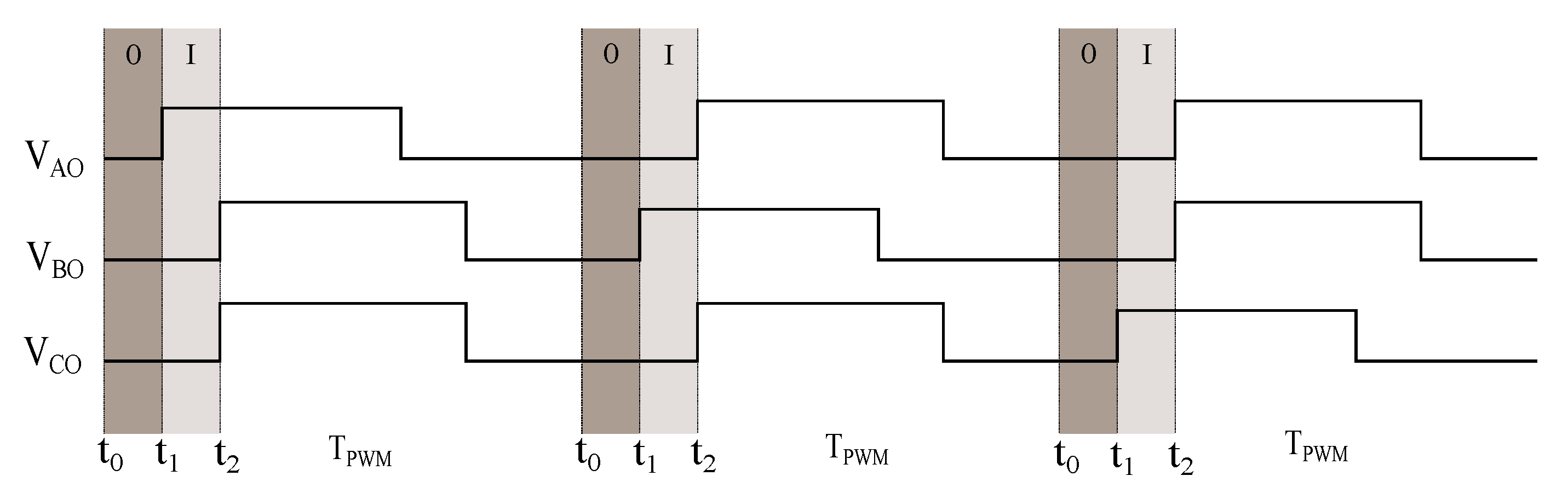
2.5. The Direct Flux Control Technique

The direct flux control technique stems from the mathematical analysis presented in the previous section. As discussed, it is necessary to measure the differential voltage $v_{NV}$ between the star-point voltage $v_{NO}$ and the virtual star-point voltage $v_{VO}$ before and after the transition of the machine between the two excitation states shown in Figure 2. For this reason, a modified edge-aligned PWM was used, as shown in Figure 7. In particular, the PWM time period $T_{PWM}$ starts at time $t_0$. One phase was then switched to the bus voltage at the time instant $t_1$ and, finally, the driving excitation according to standard edge-aligned PWM started at the time instant $t_2$. During these two states of excitation, measurements can be performed. In order to obtain the ${\mathbf{\Gamma }}_{abc}$, two measurements were performed, one per each excitation state, at the time instants $t_{m0}$ and $t_{m1}$, as shown in Figure 8, where the response of the star-point voltage, the virtual star-point voltage, and their difference is shown and the measuring time instants are indicated. The difference between these two quantities was then calculated, therefore, a new measurement of the quantities ${\mathbf{\Gamma }}_{abc}$ was obtained for each PWM period. Measurements can be performed by means of standard electronics consisting of voltage dividers and operational amplifiers-based voltage followers.

3. Experimental Validation

In the previous section, conditions on the existence of extractable rotor position information in the ${\mathbf{\Gamma }}_{\alpha \beta \gamma }$ signals have been given. Moreover, it has been shown how a typical PMSM having inductances fluctuating twice with the rotor position, (see Equation (35)), provides measured signals characterized by a second and a fourth harmonic, (Equations (36) and (37)). The obtained position error was also modeled in relation to the amplitudes a and b of the second and fourth harmonics of ${\Gamma }_{\alpha }$ and ${\Gamma }_{\beta }$, respectively. In this section, two different experimental validations are conducted. Firstly, in order to verify the proposed model, the ${\mathbf{\Gamma }}_{abc}$ signals over a full electrical period of a test machine driven by means of external high-precision rotation stage were measured by means of the direct voltage measurement (DVM) technique presented in [23]. Thus, ${\mathbf{\Gamma }}_{\alpha \beta \gamma }$ was calculated and, by means of the FFT (Fast Fourier Transform), the amplitudes a and b of the second and fourth harmonics were obtained. By means of these values, the position error was predicted and compared to the measured one. Secondly, in order to test the dynamic behavior of the proposed technique, a field oriented control was implemented and the test machine was driven under both no load and load condition to its nominal speed.

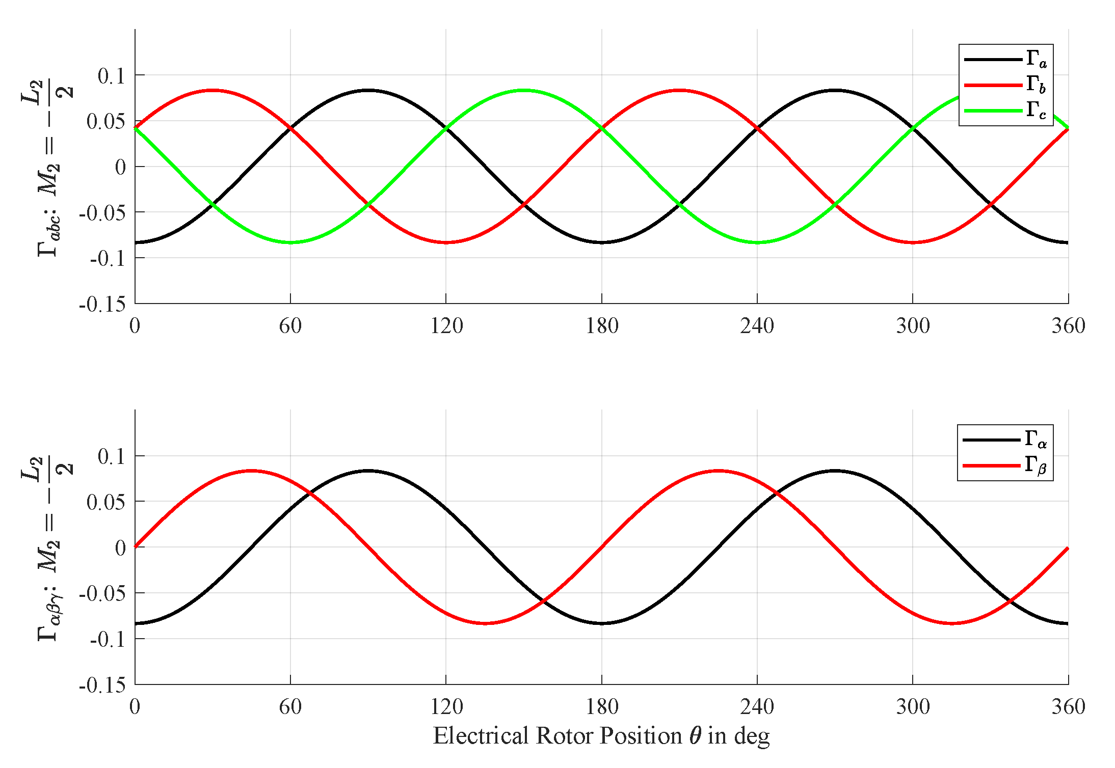
3.1. Measurement and Validation of ${\mathbf{\Gamma }}_{abc}$

The test bench used for this experimental validation was composed of a custom PMSM whose rotor was coupled to a precision rotation stage driven by a servo controller as shown in Figure 9. The rotation stage had a resolution of 6.3 μrad and a maximum rotation speed of 16 $\frac{\mathrm{deg}}{\mathrm{s}}$. In order to perform the measurement of ${\mathbf{\Gamma }}_{abc}$, an electronic board based on a 32-bit microcontroller, a three-phase inverter, and the necessary sensing circuitry was developed. The acquired measurements were transmitted to a PC over USB communication and recorded.

The machine under test was a low-power outer rotor PMSM whose main parameters are listed in

Table 2. Parameters of the custom PMSM.

Motor Parameters	Values
Phase resistance	1.1 $\Omega$
d-axis inductance	394 $\mathsf{\mu }\mathrm{H}$
q-axis inductance	475 $\mathsf{\mu }\mathrm{H}$
Pole pairs	8
Torque constant	0.1186 $\frac{\mathrm{Nm}}{\mathrm{A}}$
Nominal voltage	24 V
Nominal current	1.5 A
Nominal speed	500 rpm
Nominal torque	200 mNM

. A cross-section of the machine is shown in Figure 10. The machine had an outer diameter of 42 mm, a stacklength of 30 mm and an airgap of $0.4$ mm. Moreover, it was made of 18 stator slots and 16 poles and was equipped with three phase single layer concentrated windings in a star configuration. Finally, the permanent magnets were made of neodymium (NdFeB) and were 90% embedded into the laminated rotor core.

In order to measure ${\mathbf{\Gamma }}_{abc}$ over a full electrical period, the PMSM under test was rotated by the rotation stage at a speed of 0.125 mechanical degrees per second that corresponds to 1 electrical degree per second given that the number of pole pairs is 8. A dedicated electronics implementing direct voltage measurement, [23], was used by applying 50% dutycycles, thus no average torque was produced by the PMSM. At the top part of Figure 11 the obtained measurements are shown, while at the bottom part the calculated ${\mathbf{\Gamma }}_{\alpha \beta \gamma }$ are displayed over the reference electrical position provided by the high-precision rotation stage encoder. It must be noted that ${\mathbf{\Gamma }}_{abc}$ was normalized.

The measured ${\mathbf{\Gamma }}_{abc}$ was composed of three signals whose amplitudes were similar (1.744, 1.774, 1.765 for ${\Gamma }_a$, ${\Gamma }_b$, and ${\Gamma }_c$, respectively) but with different mean values (−0.052, 0.028, 0.034). This can be observed in Figure 11, where ${\Gamma }_a$ clearly shows a lower mean value than the other two signals. This can be explained by asymmetries of the machine. In Equation (34), all self and mutual inductances are considered as having the same mean value and fluctuation amplitude. This is not always the case, especially for small-sized machines. It must be remarked that the PMSM under test was a low-power prototype machine, thus technological tolerances are to be expected.

In order to verify the accuracy of the mathematical description in Equations (36) and (37), the FFT of ${\Gamma }_{\alpha }$ and ${\Gamma }_{\beta }$ was calculated. Figure 12 reports the obtained amplitudes and phases for both signals. As one can easily observe, the obtained results match closely with those expected from the mathematical description. In fact, the presence of the 2nd and 4th harmonics is evident, as well as the presence of a few higher order harmonics. Moreover, one can see that a variation can be observed in the amplitudes of the 2nd and 4th harmonics. In detail, the mismatch between the amplitude of the 2nd harmonic between ${\Gamma }_{\alpha }$ and ${\Gamma }_{\beta }$ is 3.5%, while the mismatch related to the 4th harmonic is 17%. Such deviations can be justified by the non-perfect symmetry of the machine under test, due to the manufacturing process. It has to be remarked, in fact, that the proposed mathematical model has been developed assuming a symmetric inductance matrix.

The obtained FFT allows the determination, per inspection, of the values of a and b used in Equations (36) and (37). Since there is a deviation in the amplitude of the 2nd and 4th harmonics for ${\Gamma }_{\alpha }$ and ${\Gamma }_{\beta }$, a was determined as the mean value between the amplitudes of the 2nd harmonics of ${\Gamma }_{\alpha }$ and ${\Gamma }_{\beta }$ while b was determined as the mean value between the amplitudes of the 4th harmonics. The obtained values are $a=-0.832$ and $b=0.074$. Based on these values, ${\Gamma }_{\alpha }$ and ${\Gamma }_{\beta }$ were numerically calculated. Figure 13 shows a comparison between the measured ${\Gamma }_{\alpha }$ and ${\Gamma }_{\beta }$ and their model. As one can see, the mathematical description and the identified parameters match the measured data with a maximum percentage error of 5.8% for ${\Gamma }_{\alpha }$ and of 5.3% for ${\Gamma }_{\beta }$.

After measuring ${\mathbf{\Gamma }}_{\alpha \beta \gamma }$, Equation (25) was used to obtain the measured angle $\chi$. As described by Equation (43), considered that $a<0$ according to identification, the electrical position was as expected, i.e., it is equal to $-2\theta -f(\theta )$. The measured DFC position, $\widehat{\theta }$, can be evaluated by means of Equation (45). Moreover, based on the identified values of a and b performed on the signals ${\Gamma }_{\alpha \beta \gamma }$, it is possible to calculate, according to the model, the angles $\chi$ and $\widehat{\theta }$ as well as the term $f\left(\theta \right)$. Figure 14 shows a comparison between the measured angles $\chi$ and $\widehat{\theta }$ and the calculated ones with respect to the position given by the high-precision encoder of the rotating stage. At the bottom of the figure, the divergence between the measured error and the calculated error is shown. As one can observe, both measured and calculated position errors ($f(\theta )$) are zero at angles multiple of $\frac{\pi }{6}$. Moreover, the measured $f(\theta )$ is limited within the range −3.7 to 3.9 degrees. The calculated $f(\theta )$, instead, is limited within $\pm 5.1$ degrees. The deviation between the measured and the calculated $f(\theta )$ is in the range of $\pm 4$ degrees and that can be explained by considering the fact that the measured ${\mathbf{\Gamma }}_{\alpha \beta \gamma }$ also present the harmonics of a higher order and a slight deviation from its mathematical description. Thus, such higher order harmonics would need to be considered in order to provide a more accurate description of $f(\theta )$. Nevertheless, such accuracy goes out of the scope of this work and it is, therefore, not considered here.

A decrease in performance of the dynamic behavior of the controlled PMSM has to be expected when an error in the electrical position error is present and it is dependent on the particular machine. More in detail, the controlled current in the machine, when no flux-weakening is desired, requires only the current along the q-axis to be controlled for torque generation. An error in the electrical position will result in a lower current along the q-axis, thus less generated torque, but also a component along the d-axis, having the effect of flux-weakening. A deeper and extensive investigation on this topic can be found in [32]. Nevertheless, for the particular machine under test, the obtained position error does not limit the control of the machine within the range of operation defined by its nominal speed and torque, as shown in the next section.

3.2. Validation of the Proposed Technique under Dynamic Conditions

In order to verify the proposed technique under dynamic conditions, a different test-bench has been utilized. In this case, the same machine as in the previous section has been coupled to a servo-motor used for application of load-torques and to a high-precision 18-bit encoder as shown in Figure 15. The test machine has been controlled in current and speed by using a standard field oriented control technique and the estimated position obtained by the DFC technique is used. The encoder has been used for validation of the results.

In order to have an estimation of the cross-coupling magnetic saturation effect, the rotor of the PMSM under test was locked to zero degrees and a $q$-axis current ranging between $-1.5$ A and $1.5$ A was driven in order to observe the error in the estimated DFC position given by the stator flux. The result is shown in Figure 16, where one can observe that the error is confined within $\pm 3$ degrees and is almost linearly dependent on the q-axis current.

The PMSM under test has been driven up to its nominal speed of 500 $\mathrm{rpm}$ in both directions without any load applied to the machine. Figure 17 shows the speeds measured by the encoder and by the DFC technique as well as the controlled currents along the d- and q-axis. The d-axis current was controlled to zero while the q-axis current was controlled for torque generation. One can observe how the speed measured by means of the DFC technique exhibits oscillations. This is due to the presence of the harmonic error in the estimated position described in the previous section, Equation (44). Figure 18 shows a zoom during the speed reversal. The presence of this oscillation in the estimated electrical rotor position is visible in Figure 19, where ${\mathbf{\Gamma }}_{abc}$ and ${\mathbf{\Gamma }}_{\alpha \beta \gamma }$ were shown during the inversion of the speed direction. Moreover, one can observe that also the controlled currents oscillate since the estimated rotor position is used for control.

Since the analysis in this work does not consider the effect of magnetic saturation, the same experiment was conducted by applying two load-torques to the test machine of 150 and 200 $\mathrm{mNm}$, respectively. Figure 20 and Figure 21 show the machine speed measured with the DFC technique as well as with the encoder together with the controlled d- and q-axis currents under loaded conditions. ${\mathbf{\Gamma }}_{abc}$, ${\mathbf{\Gamma }}_{\alpha \beta \gamma }$, and a comparison between the estimated rotor position and the measured one are shown in Figure 22 and Figure 23. Figure 24 and Figure 25 show a zoom on the speed reversal operation. In this case, the technique was capable of driving the machine up to its nominal speed and magnetic saturation had little effect on the obtained performance. Moreover, the presence of the estimation error induces oscillations on the electrical speed obtained with the proposed technique as well as on the measured currents. The amplitude of the speed oscillation was constant among the conducted experiments, as this is given by the amplitude of the ripple $f\left(\theta \right)$ present on the estimated position that was constant at a given speed. In particular, the obtained oscillation amplitude is $\pm 50$ RPM. The presence of this oscillation tendentially degrades the performance of the dynamic behavior of the machine. Nevertheless, the machine was controlled by means of two standard PI controllers, both for the speed and the current control loops. Due to the integral action, such controllers have a low-pass filter effect on the error signal. The experiments, in fact, demonstrated that the implemented field-oriented control is still capable, in front of such oscillations, to control the machine under test to nominal speed and current.

From the experiments, it is evident that, notwithstanding the presence of an electrical position error, the controllers are capable of driving the machine under test in the nominal speed and load range. Nevertheless, the electrical rotor position error increases with respect to what has been measured in the experiment shown in Figure 16, passing from $\pm 3$ degrees at zero speed to $\pm 4.5$ degrees at 500 RPM. The reason lies in the dependency of the machine phase inductances on the driven current and its derivative, that, in a synchronous machine increases with its rotational speed, due to the nonlinear nature of the magnetic stator material. Thus, rotational speed affects the estimated rotor position because of a variation of the matrix ${\mathbf{L}}_{abc}$. It has to be remarked that the back-EMF is not responsible of the observed behavior since it is eliminated inherently by the DFC technique that, in this case, is based on measurements couples that are taken within an interval of 1 $\mathsf{\mu }$s during which the back-EMF can be considered constant. Therefore, when subtracting the first measurement from the second one, the back-EMF is eliminated.

4. Conclusions and Outlooks

This work proposes an analysis for the application of the direct flux control technique to PMSMs. Although this technique is based on the exploitation of machine anisotropies, it differs from standard high-frequency injection methods by the fact that does not rely on the measured currents but rather on the measurement of the star-point voltage. As discussed, these approaches are fundamentally different in the information that is used to extract the electrical rotor position. For this reason, this work has shown under which condition the DFC technique can be used successfully. In particular, two equivalent conditions have been demonstrated, one derived in the stator reference frame and one in the rotor reference frame. In the particular case of PMSMs, this leads to the condition $L_2\ne M_2$. Moreover, an analysis of the signals measured by the DFC technique (${\mathbf{\Gamma }}_{abc}$) and of the estimated electrical position ($\chi$) was conducted. In particular, it was shown that the measured signals ${\mathbf{\Gamma }}_{\alpha \beta \gamma }$ in the stator reference frame introduce a 4th harmonic that induces a position error that is affected by a 6th nonlinear harmonic, whose bounds have been analytically determined. Moreover, the condition that leads to canceling this error was found and presented, i.e., $L_2=-\frac{M_2}{2}$. Such condition can be used during the design of a PMSM that is intended to be driven by such technique. Experimental investigations have validated the proposed mathematical model and proven the capability of this technique to operate up to the nominal speed and load of a test machine. Nevertheless, due to the electrical position error, oscillations in the estimated speed are present. The presented analysis has not considered the effect of cross-coupling magnetic saturation effect or the presence of higher-order harmonics of the machine phase inductances. In future works, a deeper investigation on their effect on the estimated rotor position will be conducted by means of field distribution simulations and by elaborating a more complete mathematical description. It is also of interest to investigate techniques capable of compensating for the position error in order to obtain a more precise estimated electrical rotor position and speed.

References

1. Yang, Z.; Shang, F.; Brown, I.P.; Krishnamurthy, M. Comparative Study of Interior Permanent Magnet, Induction, and Switched Reluctance Motor Drives for EV and HEV Applications. IEEE Trans. Transp. Electrif. 2015, 1, 245–254. [Google Scholar] [CrossRef]
2. Xu, D.; Wang, B.; Zhang, G.; Wang, G.; Yu, Y. A review of sensorless control methods for AC motor drives. CES Trans. Electr. Mach. Syst. 2018, 2, 104–115. [Google Scholar] [CrossRef]
3. Schrödl, M. Sensorless Control of A. C. Machines; Fortschritt-Berichte VDI: Reihe 21, Elektrotechnik; 117; VDI-Verl.: Düsseldorf, Germany, 1992; Volume 117. [Google Scholar]
4. Schrödl, M. Sensorless control of AC machines at low speed and standstill based on the “INFORM” method. In Proceedings of the IAS ’96. Conference Record of the 1996 IEEE Industry Applications Conference Thirty-First IAS Annual Meeting, San Diego, CA, USA, 6–10 October 1996; Volume 1, pp. 270–277. [Google Scholar] [CrossRef]
5. Lorenz, R.D. Transducerless Position and Velocitv Estimation in Induction and Salient AC Machines. IEEE Trans. Ind. Appl. 1995, 31, 240–247. [Google Scholar]
6. Corley, M.; Lorenz, R. Rotor position and velocity estimation for a salient-pole permanent magnet synchronous machine at standstill and high speeds. IEEE Trans. Ind. Appl. 1998, 34, 784–789. [Google Scholar] [CrossRef]
7. Linke, M.; Kennel, R.; Holtz, J. Sensorless position control of permanent magnet synchronous machines without limitation at zero speed. In Proceedings of the IEEE 2002 28th Annual Conference of the Industrial Electronics Society (IECON 02), Sevilla, Spain, 5–8 November 2002; Volume 1, pp. 674–679. [Google Scholar] [CrossRef]
8. Linke, M.; Kennel, R.; Holtz, J. Sensorless speed and position control of synchronous machines using alternating carrier injection. In Proceedings of the IEEE International Electric Machines and Drives Conference (IEMDC’03), Madison, WI, USA, 1–4 June 2003; Volume 2, pp. 1211–1217. [Google Scholar] [CrossRef]
9. Landsmann, P.; Paulus, D.; Stolze, P.; Kennel, R. Saliency based encoderless predictive torque control without signal injection. In Proceedings of the 2010 International Power Electronics Conference - ECCE ASIA, Sapporo, Japan, 21–24 June 2010; pp. 3029–3034. [Google Scholar] [CrossRef]
10. Paulus, D.; Landsmann, P.; Kennel, R. Sensorless field- oriented control for permanent magnet synchronous machines with an arbitrary injection scheme and direct angle calculation. In Proceedings of the 2011 Symposium on Sensorless Control for Electrical Drives, Birmingham, UK, 1–2 September 2011; pp. 41–46. [Google Scholar] [CrossRef]
11. Paulus, D.; Landsmann, P.; Kennel, R. Saliency based sensorless field- oriented control for permanent magnet synchronous machines in the whole speed range. In Proceedings of the 3rd IEEE International Symposium on Sensorless Control for Electrical Drives (SLED 2012), Milwaukee, WI, USA, 21–22 September 2012; pp. 1–6. [Google Scholar] [CrossRef]
12. Consoli, A.; Scarcella, G.; Testa, A. A new zero-frequency flux-position detection approach for direct-field-oriented-control drives. IEEE Trans. Ind. Appl. 2000, 36, 797–804. [Google Scholar] [CrossRef]
13. Consoli, A.; Scarcella, G.; Testa, A.; Lipo, T.A. Air-Gap Flux Position Estimation of Inaccessible Neutral Induction Machines by Zero-Sequence Voltage. Electr. Power Components Syst. 2002, 30, 77–88. [Google Scholar] [CrossRef]
14. Holtz, J.; Pan, H. Elimination of saturation effects in sensorless position controlled induction motors. In Proceedings of the Conference Record of the 2002 IEEE Industry Applications Conference—37th IAS Annual Meeting (Cat. No.02CH37344), Pittsburgh, PA, USA, 13–18 October 2002; Volume 3, pp. 1695–1702. [Google Scholar] [CrossRef]
15. Holtz, J.; Pan, H. Acquisition of Rotor Anisotropy Signals in Sensorless Position Control Systems. IEEE Trans. Ind. Appl. 2004, 40, 1379–1387. [Google Scholar] [CrossRef]
16. Holtz, J. Sensorless Control of Induction Machines—With or Without Signal Injection? IEEE Trans. Ind. Electron. 2006, 53, 7–30. [Google Scholar] [CrossRef] [Green Version]
17. Consoli, A.; Scarcella, G.; Tutino, G.; Testa, A. Zero frequency rotor position detection for synchronous PM motors. In Proceedings of the 2000 IEEE 31st Annual Power Electronics Specialists Conference—Conference Proceedings (Cat. No.00CH37018), Galway, Ireland, 23 June 2000; Volume 2, pp. 879–884. [Google Scholar] [CrossRef]
18. Strothmann, R. Fremderregte Elektrische Maschine. EP Patent EP1005716B1, 14 November 2001. [Google Scholar]
19. Thiemann, P.; Mantala, C.; Mueller, T.; Strothmann, R.; Zhou, E. Direct Flux Control (DFC): A New Sensorless Control Method for PMSM. In Proceedings of the 2011 46th International Universities’ Power Engineering Conference, Soest, Germany, 5–8 September 2011. [Google Scholar]
20. Mantala, C. Sensorless Control of Brushless Permanent Magnet Motors. Ph.D. Thesis, University of Bolton, Bolton, UK, 2013. [Google Scholar]
21. Grasso, E.; Merl, D.; Nienhaus, M. Verfahren und Vorrichtung zum Bestimmen einer Läuferlage eines Läufers einer elektronisch kommutierten elektrischen Maschine. DE Patent DE102016117258A1, 21 March 2018. [Google Scholar]
22. Merl, D.; Grasso, E.; Schwartz, R.; Nienhaus, M. A Direct Flux Observer based on a Fast Resettable Integrator Circuitry for Sensorless Control of PMSMs. In Proceedings of the ACTUATOR 2018; 16th International Conference on New Actuators, Bremen, Germany, 25–27 June 2018; p. 4. [Google Scholar]
23. Grasso, E.; Mandriota, R.; König, N.; Nienhaus, M. Analysis and Exploitation of the Star-Point Voltage of Synchronous Machines for Sensorless Operation. Energies 2019, 12, 4729. [Google Scholar] [CrossRef] [Green Version]
24. Iwaji, Y.; Kokami, Y.; Kurosawa, M. Position-sensorless control method at low speed for permanent magnet synchronous motors using induced voltage caused by magnetic saturation. In Proceedings of the 2010 International Power Electronics Conference (ECCE ASIA), Sapporo, Japan, 21–24 June 2010; pp. 2238–2243. [Google Scholar] [CrossRef]
25. Iwaji, Y.; Takahata, R.; Suzuki, T.; Aoyagi, S. Position Sensorless Control Method at Zero-Speed Region for Permanent Magnet Synchronous Motors Using the Neutral Point Voltage of Stator Windings. IEEE Trans. Ind. Appl. 2016, 52, 4020–4028. [Google Scholar] [CrossRef]
26. Hara, T.; Aoyagi, S.; Ajima, T.; Iwaji, Y.; Takahata, R.; Sugiyama, Y. Neutral Point Voltage Model of Stator Windings of Permanent Magnet Synchronous Motors with Magnetic Asymmetry. In Proceedings of the 2018 XIII International Conference on Electrical Machines (ICEM), Alexandroupoli, Greece, 3–6 September 2018; pp. 1611–1616. [Google Scholar] [CrossRef]
27. Xu, P.; Zhu, Z. Novel Carrier Signal Injection Method Using Zero Sequence Voltage for Sensorless Control of PMSM Drives. IEEE Trans. Ind. Electron. 2015, 63. [Google Scholar] [CrossRef]
28. Xu, P.L.; Zhu, Z.Q. Novel Square-Wave Signal Injection Method Using Zero-Sequence Voltage for Sensorless Control of PMSM Drives. IEEE Trans. Ind. Electron. 2016, 63, 7444–7454. [Google Scholar] [CrossRef]
29. Schuhmacher, K.; Kleen, S.; Nienhaus, M. Comparison of Anisotropy Signals for Sensorless Control of Star-Connected PMSMs. In Proceedings of the 2019 IEEE 10th International Symposium on Sensorless Control for Electrical Drives (SLED), Turin, Italy, 9–10 September 2019; pp. 1–6. [Google Scholar] [CrossRef]
30. Raja, R.; Sebastian, T.; Wang, M. Online Stator Inductance Estimation for Permanent Magnet Motors Using PWM Excitation. IEEE Trans. Transp. Electrif. 2019, 5, 107–117. [Google Scholar] [CrossRef]
31. Poltschak, F.; Amrhein, W. Influence of winding layout of PMSM on inductance and its impact on suitability for sensorless vector control. In Proceedings of the SPEEDAM 2010, Pisa, Italy, 14–16 June 2010; pp. 1002–1007. [Google Scholar] [CrossRef]
32. Gächter, J.; Hirz, M.; Seebacher, R. The effect of rotor position errors on the dynamic behavior of field-orientated controlled PMSM. In Proceedings of the 2017 IEEE International Electric Machines and Drives Conference (IEMDC), Miami, FL, USA, 21–24 May 2017; pp. 1–8. [Google Scholar] [CrossRef]
Figure 1. Virtual star point.
Energies 13 01453 g001
Figure 2. Transition between the machine state excitation 0 to 1. X, Y, and Z represent generic phases belonging to the set A , B , C .
Energies 13 01453 g002
Figure 3. Comparison between Γ a b c and Γ α β γ signals in dependence of L Δ variations.
Energies 13 01453 g003
Figure 4. Comparison of the estimated rotor position to the real angle θ in dependence of L Δ variations.
Energies 13 01453 g004
Figure 5. Γ α and Γ β signals for M 2 = L 2 2 .
Energies 13 01453 g005
Figure 6. Comparison of the estimated rotor position to the real angle θ for M 2 = L 2 2 .
Energies 13 01453 g006
Figure 7. Modified edge-aligned PWM pattern used for measurement of the v N V voltage for the DFC technique.
Energies 13 01453 g007
Figure 8. Simulated response of the star-point voltages during the machine excitation states 0 and I.
Energies 13 01453 g008
Figure 9. Test bench used for experimental validation.
Energies 13 01453 g009
Figure 10. Cross-section of the permanent magnet synchronous machine (PMSM) under test.
Energies 13 01453 g010
Figure 11. Measured and normalized Γ a b c and Γ α β γ .
Energies 13 01453 g011
Figure 12. FFT amplitudes and phases of the measured and normalized Γ α and Γ β .
Energies 13 01453 g012
Figure 13. Comparison between measured and normalized Γ α and Γ β and the model.
Energies 13 01453 g013
Figure 14. Measured position and calculated position with respect to the high-precision encoder represented on the x-axis. From top to bottom: Measured and calculated angle χ . Measured and calculated angle θ ^ . Measured and calculated position error. Difference between the measured position and the calculated position.
Energies 13 01453 g014
Figure 15. Test bench used for experimental validation.
Energies 13 01453 g015
Figure 16. Estimated electrical position error over q-axis current.
Energies 13 01453 g016
Figure 17. Acceleration test at no load of the PMSM to nominal speed.
Energies 13 01453 g017
Figure 18. Acceleration test at no load of the PMSM to nominal speed with zoom on the speed inversion.
Energies 13 01453 g018
Figure 19. Γ a b c , Γ α β γ , and comparison of the estimated electrical rotor position to the measured one during inversion at no load.
Energies 13 01453 g019
Figure 20. Acceleration test of the PMSM to nominal speed at 150 mNm load-torque.
Energies 13 01453 g020
Figure 21. Acceleration test of the PMSM to nominal speed at 200 mNm load-torque.
Energies 13 01453 g021
Figure 22. Γ a b c , Γ α β γ , and comparison of the estimated electrical rotor position to the measured one during inversion at 150 mNm load-torque.
Energies 13 01453 g022
Figure 23. Γ a b c , Γ α β γ , and comparison of the estimated electrical rotor position to the measured one during inversion at 200 mNm load-torque.
Energies 13 01453 g023
Figure 24. Acceleration test of the PMSM to nominal speed at 150 mNm load-torque with zoom on the speed inversion.
Energies 13 01453 g024
Figure 25. Acceleration test of the PMSM to nominal speed at 200 mNm load-torque with zoom on the speed inversion.
Energies 13 01453 g025