Electrical Characterization of a New Crosslinked Copolymer Blend for DC Cable Insulation

Abstract

To design reliable high voltage cables, clean materials with superior insulating properties capable of operating at high electric field levels at elevated temperatures are required. This study aims at the electrical characterization of a byproduct-free crosslinked copolymer blend, which is seen as a promising alternative to conventional peroxide crosslinked polyethylene currently used for high voltage direct current cable insulation. The characterization entails direct current (DC) conductivity, dielectric response and surface potential decay measurements at different temperatures and electric field levels. In order to quantify the insulating performance of the new material, the electrical properties of the copolymer blend are compared with those of two reference materials; i.e., low-density polyethylene (LDPE) and peroxide crosslinked polyethylene (XLPE). It is found that, for electric fields of 10–50 kV/mm and temperatures varying from 30 °C to 70 °C, the DC conductivity of the copolymer blend is in the range of 10⁻¹⁷–10⁻¹³ S/m, which is close to the conductivity of crosslinked polyethylene. Furthermore, the loss tangent of the copolymer blend is about three to four times lower than that of crosslinked polyethylene and its magnitude is on the level of 0.01 at 50 °C and 0.12 at 70 °C (measured at 0.1 mHz and 6.66 kV/mm). The apparent conductivity and trap density distributions deduced from surface potential decay measurements also confirmed that the new material has electrical properties at least as good as currently used insulation materials based on XLPE (not byproduct-free). Thus, the proposed byproduct-free crosslinked copolymer blend has a high potential as a prospective insulation medium for extruded high voltage DC cables.

1. Introduction

High voltage direct current (HVDC) cables play a crucial role in modern power transmission systems allowing for transporting bulk energy over long distances with low transmission losses. In parallel with the development of new HVDC technologies, cable insulations have undergone extensive material development to meet the requirements of increased operating voltage levels, which nowadays reach 640 kV [1,2,3,4]. The choice of materials for insulation of such cables has mainly concentrated on crosslinked polyethylene (XLPE) due to the optimal combination of its electrical insulating performance, thermomechanical properties and chemical stability [5,6]. In the case of power cable applications, the most widely used crosslinking method is peroxide crosslinking using dicumyl peroxide (DCP), where the degree of crosslinking is chosen based on the required electromechanical properties of the material [5]. One major problem associated with this method is the presence of unwanted byproducts, which have a negative impact on the electrical properties. Therefore, avoiding these byproducts would be of considerable benefit. Typically, byproducts are removed by degassing which is a time- and energy- consuming process. For instance, the degassing of the insulation of a 132-kV cable carried out at 60 °C takes about 2.5 days per mm of the insulation thickness [7]. Furthermore, the insulation of cables operating at higher voltages demands materials of extremely high purity. By today, the material manufacturing technology has reached a stage where a further increase in the cleanliness is not feasible mainly due to the high cost [3]. Despite these difficulties, researchers and developers are working on further development of XLPE for HVDC applications [1,2,3,4,5,8]. The activities in this area are mainly directed towards improving purity [9,10], adding organic additives/voltage stabilizers [11,12] and nanofillers [13,14,15,16]. Other materials such as polyethylene-based nanocomposites [5,17,18], polypropylene (PP) [19,20,21,22], ethylene-propylene rubber (EPR) [23,24] and polymer blends [25,26,27] have also received attention as potential substitutes for XLPE. Even though these materials have been found to exhibit some desired properties, e.g., ultralow conductivities [28], in-depth electrical characterization is essential before commercial HVDC applications [1,2] can be considered.

Recently, other types of copolymer blends with similar electromechanical properties to XLPE have gained interest among materials scientists [19,22,29,30,31,32,33]. For example, [19,22] investigated polyethylene-based copolymers in terms of structural, morphological, mechanical and electrical properties. In previous studies [29,30,31,32,33], we have introduced a byproduct-free crosslinking method based on click chemistry-type reactions for the development of polyethylene-based insulations. In these novel materials, there is no trace of detrimental by-products, and therefore the degassing process, which is a long and costly part of high-voltage cable manufacturing, is omitted. The most promising way to realize this type of material involves blending of two copolymers: a statistical ethylene-glycidyl methacrylate copolymer, p(E-stat-GMA), and an ethylene-acrylic acid copolymer, p(E-stat-AA) [32]. These two copolymers can be compounded/extruded at 120 to 140 °C without the risk of crosslinking. After cable extrusion, rapid crosslinking via click chemistry can be achieved at 160 °C and above. Preliminary investigations presented in [32] indicated promisingly low DC conductivities (measured with broadband dielectric spectroscopy) of the obtained materials in comparison with commonly used high voltage insulation materials (including XLPE). A proof-of-concept study included DC conductivity measurements at specific/desired operational conditions [33]. However, additional advanced electrical characterization needs to be done to shed light on the underlying charge transport mechanisms involved. This should facilitate further material development for higher voltage levels, where the conventional XLPE (not byproduct-free) shows electromechanical limitations.

This study presents an in-depth electrical characterization of the proposed copolymer blend focusing on conduction related properties. Out of five materials proposed in [32], the copolymer blend having the lowest conductivity was selected for the analysis. Here, low-density polyethylene (LDPE) and its crosslinked version XLPE were selected as reference materials. In the previous studies [32,33], electrical characterizations were limited to broadband dielectric spectroscopy at a very low electric field stress of 10 V/mm and high-voltage DC conductivity measurements at a specific condition (70 °C, 20 and 30 kV/mm). Therefore, it is important to evaluate the new material at different high-voltage conditions, which may permit to identify the underlying charge transport mechanisms. This approach helps us to design/develop an insulation material with superior electrical properties that can meet the requirements in terms of material performance for emerging applications. In the present study, the electrical characterizations were extended to different electric fields from 10 up to 50 kV/mm, in the temperature range of 30–70 °C. In addition to DC conductivity measurements, we have used other characterization methods, namely surface potential decay (SPD) and frequency domain dielectric spectroscopy (FDS) measurements, which shed light on charge transport behavior under operating conditions of high-voltage insulations. Finally, the DC conductivity and other relevant properties deduced from these experiments were analyzed to compare the performance of the proposed copolymer blend with that of two reference materials, LDPE and XLPE.

2. Materials and Samples

The studied copolymer blend, labeled as p(E-stat-GMA4.5):p(E-stat-AA3), was prepared by mixing two copolymers: an ethylene-glycidyl methacrylate copolymer p(E-stat-GMA4.5) comprising 4.5 wt% glycidyl methacrylate (GMA) and an ethylene-acrylic acid copolymer p(E-stat-AA3) comprising 3 wt% acrylic acid (AA), with a stoichiometry of 1.2:1. Specification of these copolymers can be found in [32]. The reference LDPE film was prepared from pellets of a neat LDPE grade provided by Borealis AB (see [32] for details). The other reference material, XLPE, was prepared from a LDPE grade that contains DCP provided by Nexans. The copolymer formulation was compounded for 10 min at 120 °C and finally extruded using a Xplore Micro Compounder MC5. The extruded material was first molten and shaped to film samples with desired thicknesses (0.13 and 0.3 mm) under 100 kN at 140 °C using a hot press, followed by crosslinking at 200 °C for 10 min. Both the LDPE and XLPE films were prepared at similar hot-press conditions from the pellets. The XLPE film was subjected to a further degassing procedure by keeping it in a vacuum oven at 60 °C overnight.

3. Experimental Setup and Methods

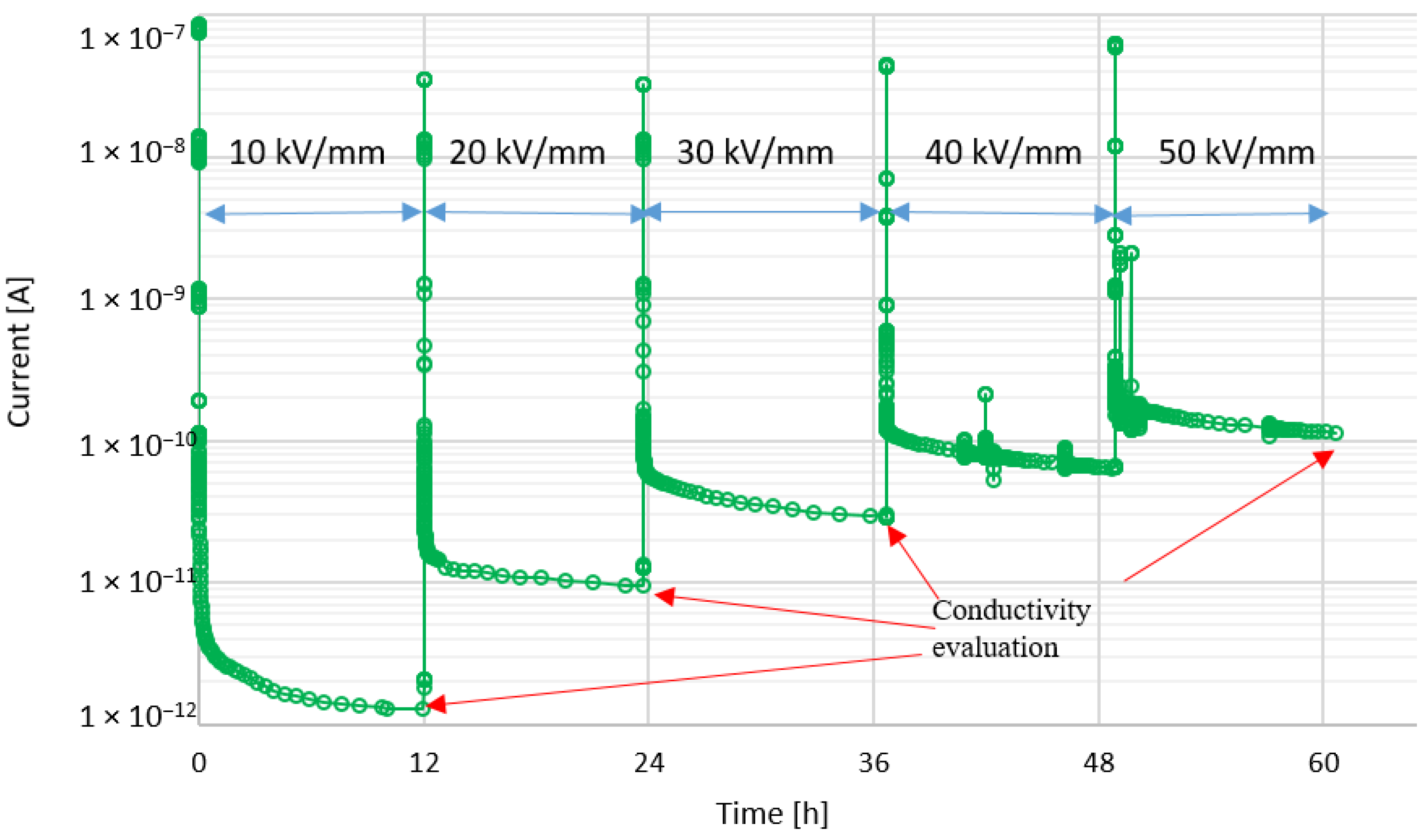
3.1. DC Conductivity Measurements

The laboratory setup used for measuring the charging current through the bulk of the sample exposed to DC voltage is illustrated in Figure 1. The high voltage (HV) electrode is connected to a 30 kV DC voltage supply through a low pass filter whereas the measuring electrode is connected to a Keithley 6517B electrometer. Diameters of the HV and measuring electrodes were 60 mm and 28 mm, respectively. A third electrode, referred as the shielding electrode, is used as a guard to divert any influence of surface to ground currents. The whole electrode arrangement is kept inside a shielded oven chamber not only for applying a specific temperature, but also to suppress the noise inherently present when measuring extremely low currents (pA and below). The Keithley electrometer was connected to a PC through General Purpose Interface Bus (GPIB) for data recording. In order to achieve better noise rejection and effective data handling, a dynamic averaging method, referred as “smart averaging”, has been used to enable simultaneous processing and recording of the data. Detail discussion about the averaging algorithm, the measuring setup and data processing can be found in [34,35].

The following experimental procedure was used for conductivity measurements. First, the electrode system with the material sample was placed in the oven and the temperature was adjusted to 30 °C. After waiting about six hours to reach a thermal steady state and to neutralize any surface/space charges (which might be present), a DC voltage of 3 kV was applied to the 0.3 mm thick film (providing the electric field strength of 10 kV/mm) and the resulting current was recorded. The duration of the voltage exposure was set to 12 h, during which the current decayed to a quasi-steady state. Immediately after 12 h, the test voltage was increased by 3 kV and it was kept constant for another 12 h. This procedure was repeated up to the voltage level of 15 kV that provided the electric field of 50 kV/mm. The same sequence was followed with the temperatures 50 °C and thereafter 70 °C. Figure 2 shows a typical recorded current during one measurement sequence for LDPE at 50 °C. Spikes in the current correspond to the contribution of displacement current due to an increase in the voltage level after 12 h steps. As shown in Figure 2, the current level at 12 h of charging was used to evaluate the DC resistivity of the sample and, hence, the conductivity of the material. Note that the stepwise voltage increase was selected due to its negligible effect on the electrical history of the material that was observed during our preliminary measurements as well as by others [36]. The measurements were performed twice with each material sample to check the repeatability. Additionally, a third measurement sequence was carried out with another sample from the same material.

3.2. Dielectric Response Measurements

Frequency Domain Spectroscopy (FDS) measurements were conducted using a commercial insulation diagnostic analyzer IDAX 300 together with a high voltage amplifier VAX020. This setup allows measuring of the dielectric response in the frequency range of 0.1 mHz to 1 kHz with a peak voltage up to 2 kV [37]. The material sample (0.3 mm thick) was inserted in the three-electrode system similar to the one used for the conductivity measurements (but with the electrodes of 60 mm in diameter). The measurements were performed at the peak voltage of 2 kV (the respective field strength 6.66 kV/mm) over the frequency range from 0.1 mHz to 1 kHz and provided real and imaginary components of the complex capacitance from which the respective components of the complex permittivity of the material were obtained. The measurements were conducted at 30, 50 and 70 °C. As measurements at 30 °C shows low reproducibility due to the low detected current, only 50 and 70 °C tests were considered for analysis.

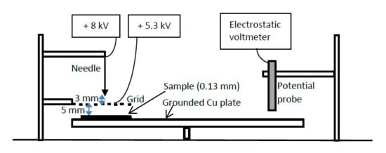
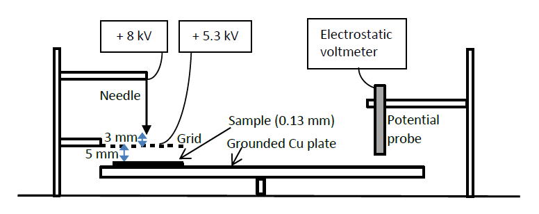
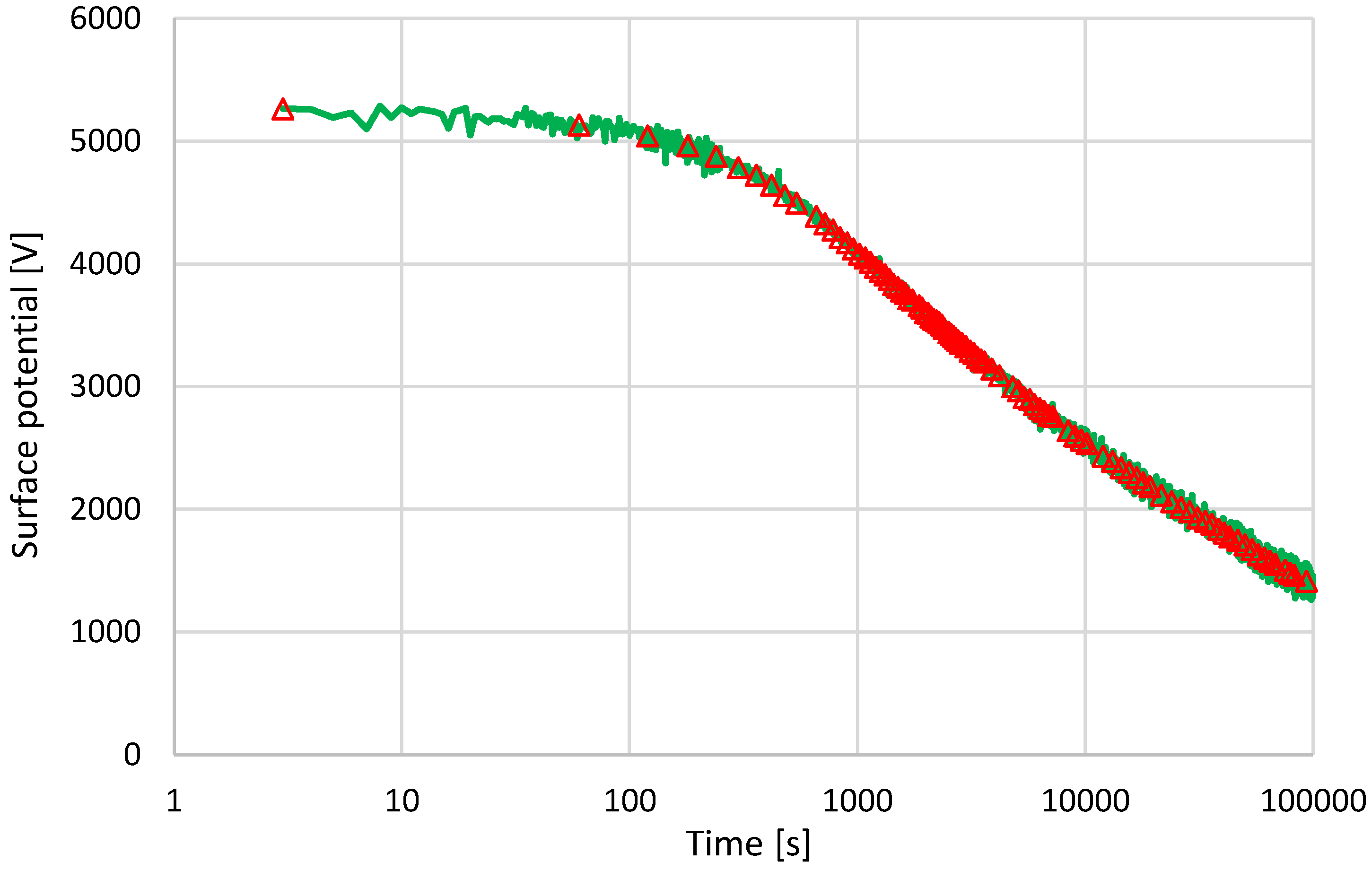
3.3. Surface Potential Decay Measurements

A schematic diagram of the setup used for surface potential decay (SPD) measurements is shown in Figure 3. The material sample was placed on a grounded copper plate mounted on a rotating table, while its upper surface was kept open to the surrounding air. The experiments were conducted in two steps. First, corona charging of the sample was achieved by applying a charging voltage to a needle (hemispherical tip of diameter 0.95 mm). A grid electrode (9 cm × 9 cm) mounted on a fixed arm between the needle and the sample and connected to a dedicated voltage supply was utilized to charge the sample surface evenly [38]. Surface-to-grid and needle-to-grid distances were 5 mm and 3 mm, respectively. Upon completion of the charging step, the table was rotated to bring the center of the sample directly under a Kelvin type electrostatic probe (Trek PN 6000B) connected to an electrostatic voltmeter (Trek 347). The surface potential was obtained by an electrostatic voltmeter and data were collected at a rate of 1 reading per second by means of a data acquisition card connected to a PC.

The measurements were conducted on 0.13 mm thick samples under ambient conditions (temperature 22–24 °C). The reason for using thinner samples compared to those for the conductivity and FDS measurements was to reach the same electric field magnitudes at feasible charging levels. Thus, each material sample was charged up to the potential magnitude of 5.3 kV that was achieved by applying the voltage of 5.3 kV between the needle and grounded plate and 8 kV to the grid. Figure 4 shows a typical surface potential decay plot recorded for a XLPE sample. It can be observed that the maximum variation of surface potential is about ±2% from the mean indicating a high signal to noise ratio. However, in order to avoid scattering in conductivity evaluations, a representative set of data points was selected by considering the decay rate. As shown in Figure 4 (by red triangular symbols) at the beginning, when decay is faster, the time between two adjacent data points is 1 min whereas the slower decays have ca. 1 h intervals.

4. Results and Discussion

4.1. DC Conductivity

DC conductivity values were calculated based on the magnitudes of the steady-state currents obtained at the end of each 12 h interval of the DC test voltage application. Figure 5 shows the variation of the DC conductivity (σ) with the electric field strength (E) obtained for three temperature levels. Note that the measurements were repeated three times for each material and test condition (i.e., electric field and temperature). The error bars on the plots represent the maximum and minimum DC conductivity values out of the three measurements, whereas the dotted lines represent a power-law type fitting for the average conductivity values:

σ_avg = aE^b,

(1)

where the fitting parameter b characterizes the field dependency of conductivity. For the curves shown in Figure 5, the values of b were in the range (1.5–3).

It can be observed that the DC conductivities of all three materials obey a power-law type dependency on electric field within the tested temperature and electric field ranges. At the lowest field and temperature (10 kV/mm, 30 °C), the conductivity values are of the order of 10⁻¹⁷ S/m. When the field and temperature reach the highest values (50 kV/mm, 70 °C), the conductivity increases by almost three orders of magnitude for all cases. These conductivity values are in good agreement with the earlier reported values for LDPE and XLPE [2,18,25,26]. The average conductivities of the copolymer blend at 30 °C are lower or nearly the same as compared to that of LDPE and XLPE for the entire range of the electric field. At 50 °C, their values are 1.3–2.6 times higher than for LDPE, but almost the same as for XLPE. The same characteristics can be observed even at 70 °C at an electric field strength of up to about 30 kV/mm. However, when considering the variations in the measured data (error bars), one can conclude that that the copolymer blend has almost the same conductivity level as XLPE for all studied temperatures (30–70 °C) and field levels (10–50 kV/mm), which cover normal operating points of high voltage power cables.

4.2. Activation Energy

As known [1,2,39], the temperature dependence of DC conductivities of polymeric insulation materials can be expressed by the Arrhenius equation.

σ = σ₀ exp(−E_A/k_BT),

(2)

where E_A is the activation energy for conduction; k_B is the Boltzmann constant; T is the temperature. The parameter σ₀ can be considered as a constant for a particular electric field strength. Thus, the activation energy can be evaluated from the slope of the Arrhenius plot log σ vs. T⁻¹. Figure 6 shows such plots drawn for the proposed material for different electric field levels. The activation energies derived for all three tested materials are presented in Figure 7 as functions of the applied electric field. It can be observed that the activation energy of LDPE is about 0.7–0.8 eV and almost independent of electric field strength. The XLPE material has higher activation energy compared to LDPE at lower electric field, but it decreases at higher fields and reaches almost the same level as for LDPE. Despite different experimental conditions and slightly different material morphologies, these activation energy levels are in reasonable agreement with the values reported in the literature [18,39,40]. As for the copolymer blend, its activation energy is slightly higher compared to XLPE while having similar field dependency. According to these results, the temperature dependence of the conductivity of the copolymer is stronger than of the two other materials. However, as the maximum variation between the activation energies of the copolymer blend and XLPE is only about 20%, for practical applications one can safely assume similar temperature dependencies for both materials. It is worth noting that a weaker temperature dependency (or lower activation energies) is desirable for DC applications since it eases control of the electric field distribution in the insulation under thermal gradients.

4.3. Dielectric Response and Losses

The results of the dielectric response measurements confirm that the real part of the complex permittivity of LDPE and XLPE is frequency independent within the range of 0.1 mHz to 1 kHz. Moreover, no temperature dependence was noticed. Similar behavior was observed for the real part of the complex permittivity of the copolymer blend. Therefore, the loss tangent tanδ (i.e. the ratio between the imaginary and real components of the permittivity) for the studied materials has the same frequency response as the imaginary component. Figure 8 shows variations of the loss tangent with frequency for 50 °C and 70 °C. As can be noticed, at frequencies higher than ~1 Hz, the loss tangent is constant, and its magnitude is the same for all materials. The loss tangent at low frequencies is increasing by this order; XLPE > copolymer > LDPE. Furthermore, at lower frequencies, its value is inversely proportional to frequency (observe-1 slope in the log-log plots) for all three tested materials indicating that the losses are dominated by conduction and no significant slow polarization processes in the materials can be observed. Therefore, at lower frequencies the insulation materials can be modeled as a lossy capacitor, i.e. a parallel RC circuit, and hence conductivity can be estimated as [41]:

$$\mathsf{\sigma }=2\mathsf{\pi }\mathrm{fd}\mathrm{C}\prime \tan \mathsf{\delta }/\mathrm{A},$$

(3)

where f is the frequency; C’ is real part of the complex capacitance; tanδ is the loss tangent; d and A are thickness and area of the sample respectively.

Using the loss tangent value at the lowest frequency of 0.1 mHz, the conductivity was evaluated and tabulated in

Table 1. Conductivity estimated from dielectric response measurements.

Material	Temperature [°C]	Loss Tangent at 6.66 kV/mm, 0.1 mHz	Conductivity from FDS at 6.66 kV/mm [fS/m]	Measured Average DC Conductivity at 10 kV/mm [fS/m]
LDPE	50	0.01	0.08	0.29
	70	0.06	0.52	1.80
XLPE	50	0.04	0.37	0.62
	70	0.40	3.96	4.42
p(E-stat-GMA4.5)	50	0.01	0.13	0.40
p(E-stat-AA3)	70	0.12	1.19	3.97

. As the measurements were performed at 2 kV peak voltage, the corresponding peak value of the electric field strength is 6.66 kV/mm. For comparison, the DC conductivities measured at 10 kV/mm (presented in Section 4.1) are also tabulated. As can be observed for 50 °C, the values of the loss tangent are close for the copolymer blend and LDPE and they are about four times lower than for XLPE. At 70 °C, the loss tangent of the copolymer blend is twice the value of LDPE and about one third of the value obtained for XLPE. Note that a low loss tangent is highly desirable for cable insulation materials from both technical and economical points of view. As for the deduced conductivity values, one may notice that they are in a reasonable agreement with the DC conductivities measured by the standard method, i.e. by using charging currents, despite of the different field strengths. This also confirms that the losses in the materials are governed by the conduction process.

4.4. Field Dependent Conductivity

As mentioned in Section 3.3, the sample surface in the SPD measurements was initially charged and then the decay of the deposited charges was monitored. In the open-circuit configuration used, the charged surface (the upper side of the sample as shown in Figure 3) is surrounded by air and is not in contact with any electrodes. Under such conditions, the surface charge decay can be attributed to three mechanisms: charge injection and conduction through the material bulk (also called bulk neutralization), charge leakage through the air-solid interface (surface conduction), and recombination of surface charges with free ions present in air (so-called gas neutralization). A detailed discussion of these mechanisms can be found in [42]. In the present experiments, as the Kelvin probe utilizing the field nullifying technique was continuously kept above the scanning surface, the electric field in its vicinity was very weak and the contribution from gas neutralization to the charge decay is considered to be negligible [43]. Furthermore, as the dielectric response measurements indicated the absence of slow polarization processes in the materials, it can be assumed that the observed potential decay is mainly due to the bulk intrinsic conduction, surface conduction, and charge injection [38,43,44]. Therefore, representing the net effect of all these mechanisms by an apparent conductivity (σ_app), the current continuity condition on the sample surface can be written as [38,43]:

$$\frac{\partial D}{\partial \mathrm{t}}+{ \mathsf{\sigma }}_{\mathrm{app}}E=0,$$

(4)

Here, E and D are the electric field strength and dielectric displacement vectors, respectively; t is time. For a uniformly charged flat dielectric sample having large dimensions compared to its thickness, this problem can be considered as one dimensional and electric field strength is defined by:

$$\mathrm{E}=\frac{\mathrm{V}\left(\mathrm{t}\right)}{\mathrm{d}},$$

(5)

where V(t) is the measured surface potential and d is thickness of the sample. Hence the apparent conductivity is given by:

$${\mathsf{\sigma }}_{\mathrm{app}}=-\frac{\mathsf{\epsilon }}{\mathrm{V}\left(\mathrm{t}\right)}\frac{\mathrm{dV}\left(\mathrm{t}\right)}{\mathrm{dt}},$$

(6)

Here, ε is the material permittivity. Due to the field dependency of the charge decay mechanism, the resulting apparent conductivity is not constant and depends on the electric field. This approach is widely used for different dielectric materials including LDPE and LDPE based nanodielectrics [38] for evaluation of the field dependent conductivity from SPD characteristics.

Figure 9 shows the field-dependent apparent conductivity deduced from the surface potential decay measurements conducted on the samples initially charged to the potential ~5.3 kV. The electric field strength used is calculated using Equation (5) and it is related to the electric field inside the material due to surface charge. A relative permittivity of 2.3 was assumed for all three materials. As very good repeatability was observed in the experiments, only one set of data was considered for this analysis. As seen from the figure, the derived conductivity dependencies on the electric field strength obey a power-law (solid lines represent power-law type fitting for the data) irrespective of the material type. The copolymer blend shows slightly lower apparent conductivities compared to LDPE for the entire field range. However, the apparent conductivity of the new material is higher than that of XLPE for lower field strength and vice versa for the higher fields. At about 20 kV/mm, the apparent conductivities of both materials are almost identical. For comparison purposes, the DC conductivities obtained from currents measured at 30 °C are also plotted in the same graph. As seen, despite of the difference in the temperatures, the apparent conductivity is within the same range as the DC conductivities of LDPE and XLPE for electric fields lower than ~20 kV/mm. However, for the field levels above ~40 kV/mm, the differences reach almost one order of magnitude. In the case of the copolymer blend, the difference between the values corresponding to low and high field regions is less pronounced compared to LDPE and XLPE. For example, at 40 kV/mm the difference is less than three times. Higher values of the apparent conductivity compared to the DC conductivity can be explained by the contributions from surface conduction and charge injection to the surface charge decay. Thus, one may suggest that the proposed material has lower or comparable surface conductivity and weaker charge injection compared to LDPE and XLPE.

4.5. Trap Energy Distributions

According to the demarcation energy model presented in [44], the energy gap between the demarcation energy level E_d (i.e. the border between filled and emptied states in the material) and the conduction band E_c is given by:

$$\mathrm{Energy} \mathrm{gap}=\left({\mathrm{E}}_{\mathrm{c}}-{\mathrm{E}}_{\mathrm{d}}\right)={\mathrm{k}}_{\mathrm{B}}\mathrm{Tln}\left(\mathrm{vt}\right),$$

(7)

Here, v is the attempt to escape frequency. Following [45] and assuming negligible re-trapping of charge carriers, the local density of traps N(E_d) can be considered as being proportional to the product of time and potential decay rate:

$$\mathrm{Trap} \mathrm{density} \mathrm{at} \mathrm{energy} {\mathrm{E}}_{\mathrm{d}}=\mathrm{N}\left({\mathrm{E}}_{\mathrm{d}}\right)\propto \mathrm{t}\frac{\mathrm{dV}}{\mathrm{dt}},$$

(8)

Based on Equations (7) and (8), a plot of t × dV/dt vs. log(t) (or energy gap) derived from a surface potential decay characteristic can provide an image of trap density distribution. This approach has been utilized to characterize trap densities in various polymeric materials including polyethylene, polypropylene, nanocomposites, as well as silicone rubbers [18,38,46,47,48]. A recent work [46] extended this model further enabling quantification of the absolute vales of the trap densities based on the decay rate.

Figure 10 illustrates an image of the trap density distributions derived for the three materials based on the measured surface potential decay characteristics. For the calculations, the attempt to escape frequency v was assumed to be equal to 10¹¹ s^–1 [38,44]. The two copolymers that we use to prepare the here studied binary blend are LDPE type materials that comprise a low amount of acrylic acid or glycidyl methacrylate comonomers [32,33]. Since the attempt to escape frequency is linked to the nanostructure of an insulation material [49] we here use the same value for the copolymer blend and LDPE to interpret our data. As it can be observed, the peak trap densities for the three materials are located close to each other in the range of 0.83 eV to 0.85 eV below the conduction band. The peak in trap density is in very good agreement with previously reported results for LDPE [26,38] and XLPE [50]. It can also be noted that the distribution for the copolymer blend is shifted to higher energies compared to LDPE and XLPE indicating the presence of deeper traps. The latter results in reduction of the conductivity, suppression of space charge accumulation and leads to higher thermal activation energies for electric conduction [1], which is in agreement with activation energies extracted from DC conductivity measurements (Figure 7).

5. Conclusions

A new byproduct-free insulation material was electrically characterized by means of DC conductivity, dielectric response and surface potential decay measurements carried out at various temperatures and electric fields. The electric insulating performance of the material was assessed and compared with reference materials, i.e. LDPE and XLPE, by analyzing the following conduction related properties: DC conductivity, activation energy for conduction, dielectric losses, field dependent apparent conductivity and trap energy distribution. It was found that the DC conductivity of the copolymer blend is on the same level as the conductivity of XLPE with an about 20% higher thermal activation energy. Further, the dielectric losses of the copolymer blend at 50–70 °C is comparable with that of LDPE and about three to four times lower than XLPE. Additionally, it was observed that the contribution of surface conduction and charge injection to the apparent conductivity in the copolymer is less or, at least, comparable to that for the other two materials (LDPE and XLPE). The trap energy distribution in the new material is shifted to higher energy gaps by about 0.2 eV, indicating the presence of slightly deeper traps compared to LDPE and XLPE. Overall, it can be concluded that the proposed copolymer blend has promising electrical properties (as good as XLPE), while it is free of any byproducts associated with crosslinking. Therefore, this material is a promising choice for the insulation of high voltage components, such as HVDC cables, which demands clean insulation materials.

References

1. Li, Z.; Du, B. Polymeric insulation for high voltage DC extruded cables: Challenges and development directions. IEEE Electr. Insul. Mag. 2018, 34, 30–43. [Google Scholar] [CrossRef]
2. Zhou, Y.; Peng, S.; Hu, J.; He, J. Polymeric insulation materials for HVDC cables: Developments, challenges and future perspectives. IEEE Trans. Dielectr. Electr. Insul. 2017, 24, 1308–1318. [Google Scholar] [CrossRef]
3. Gubanski, S.M. Insulating materials for next generations of HVAC and HVDC cables. In Proceedings of the IEEE International Conference on High Voltage Engineering and Application (ICHVE), Chengdu, China, 19–22 September 2016. [Google Scholar]
4. Montanari, G.C.; Morshuis, P.H.F.; Zhou, M.; Stevens, G.C.; Vaughan, A.S.; Han, Z.; Li, D. Criteria influencing the selection and design of HV and UHV DC cables in new network applications. High Volt. 2018, 3, 90–95. [Google Scholar] [CrossRef]
5. Plesa, I.; Notingher, P.V.; Stancu, C.; Wiesbrock, F.; Schlogl, S. Polyethylene nanocomposites for Power cable insulations. Polymers 2019, 11, 24. [Google Scholar] [CrossRef] [PubMed] [Green Version]
6. Tefferi, M.; Li, Z.; Uehara, H.; Cao, Y. The correlation and balance of critical material properties for dc cable directrices. In Proceedings of the IEEE Conference on Electrical Insulation and Dielectric Phenomena (CEIDP), Cancun, Mexico, 21–24 October 2018. [Google Scholar]
7. Andrews, T.; Hampton, R.N.; Smedberg, A.; Wald, D.; Waschk, V.; Weissenberg, W. The role of degassing in XLPE power cable manufacture. IEEE Electr. Insul. Mag. 2006, 22, 5–16. [Google Scholar] [CrossRef]
8. Chen, G.; Hao, M.; Xu, Z.; Vaughan, A.; Cao, J.; Wang, H. Review of high voltage direct current cable. CSEE J. Power Energy 2015, 1, 9–21. [Google Scholar] [CrossRef]
9. Wang, S.; Chen, P.; Li, H.; Li, J.; Chen, Z. Improved DC performance of crosslinked polyethylene insulation depending on a higher purity. IEEE Trans. Dielectr. Electr. Insul. 2017, 24, 1809–1817. [Google Scholar] [CrossRef]
10. Farkas, A.; Olsson, C.; Dominguez, G.; Englund, V.; Hagstrand, P.; Nilsson, U. Development of high-performance polymeric materials for HVDC cables. In Proceedings of the 8th International Conference on Insulated Power Cables Jicable’11, Versailles, France, 19–23 June 2011. [Google Scholar]
11. Jarvid, M.; Johansson, A.; Kroon, R.; Bjuggren, J.M.; Wutzel, H.; Englund, V.; Gubanski, S.; Andersson, M.R.; Müller, C. A new application area for fullerenes: Voltage stabilizers for power cable insulation. Adv. Mater. 2015, 27, 897–902. [Google Scholar] [CrossRef]
12. Du, B.X.; Han, C.; Li, J.; Li, Z. Effect of voltage stabilizers on the space charge behavior of XLPE for HVDC cable application. IEEE Trans. Dielectr. Electr. Insul. 2019, 26, 34–42. [Google Scholar] [CrossRef]
13. Tanka, T.; Imai, T. Advances in nanodielectric materials over the past 50 years. IEEE Electr. Insul. Mag. 2013, 29, 10–23. [Google Scholar] [CrossRef]
14. Ohki, Y. Development of XLPE-insulated cable for high-voltage dc submarine transmission line (1). IEEE Electr. Insul. Mag. 2013, 29, 65–67. [Google Scholar] [CrossRef]
15. Ohki, Y. Development of XLPE-insulated cable for high-voltage dc submarine transmission line (2). IEEE Electr. Insul. Mag. 2013, 29, 85–87. [Google Scholar] [CrossRef]
16. Watanabe, C.; Itou, Y.; Sasaki, H.; Murata, Y.; Suizu, M.; Sakamaki, M.; Watanabe, M.; Katakai, S. Practical application of ±250 kV DC XLPE cable for Hokkaido-Honshu HVDC link. Electr. Eng. Jpn 2015, 191, 64–75. [Google Scholar] [CrossRef]
17. Pourrahimi, A.M.; Olsson, T.; Hedenqvist, M.S. The role of interfaces in polyethylene-metal-oxide nanocomposites for ultra high voltage insulating materials. Adv. Mater. 2018, 30, 1703624. [Google Scholar] [CrossRef]
18. Hoang, A.T.; Pallon, L.; Liu, D.; Serdyuk, Y.V.; Gubanski, S.M.; Gedde, U.W. Charge transport in LDPE nanocomposites part I—experimental approach. Polymers 2016, 8, 173–198. [Google Scholar] [CrossRef] [Green Version]
19. Meng, P.; Zhou, Y.; Yuan, C.; Li, Q.; Liu, J.; Wang, H.; Hu, J.; He, J. Comparisons of different polypropylene copolymers as potential recyclable HVDC cable insulation materials. IEEE Trans. Dielectr. Electr. Insul. 2019, 26, 674–680. [Google Scholar] [CrossRef]
20. Zhou, Y.; Hu, J.; Dang, B.; He, J. Mechanism of highly improved electrical properties in polypropylene by chemical modification of grafting maleic anhydride. J. Phys. D Appl. Phys. 2016, 49, 415301. [Google Scholar] [CrossRef]
21. Dang, B.; He, J.L.; Hu, J.; Zhou, Y. Large improvement in trap level and space charge distribution of polypropylene by enhancing the crystalline-amorphous interfaces effect in blends. Polym. Int. 2016, 65, 371–379. [Google Scholar] [CrossRef]
22. Huang, X.Y.; Fan, Y.Y.; Zhang, J.; Jiang, P.K. Polypropylene based thermoplastic polymers for potential recyclable HVDC cable insulation applications. IEEE Trans. Dielectr. Electr. Insul. 2017, 24, 1446–1456. [Google Scholar] [CrossRef]
23. Tefferi, M.; Li, Z.; Cao, Y.; Uehara, H.; Chen, Q. Novel EPR-Insulated DC cables for future multi-terminal MVDC integration. IEEE Electr. Insul. Mag. 2019, 35, 20–27. [Google Scholar] [CrossRef]
24. Sellick, R.L.; Sullivan, J.S.; Chen, Q.; Calebrese, C. Future improvements to HVDC cables through new cable insulation materials. In Proceedings of the 13th IET International Conference on AC and DC Power Transmission (ACDC), Manchester, UK, 14–16 February 2017. [Google Scholar]
25. Hosier, I.L.; Vaughan, A.S.; Pye, A.; Stevens, C. Polymer Blends for HVDC Applications. In Proceedings of the IEEE International Conference on Dielectrics (ICD), Budapest, Hungary, 1–5 July 2018. [Google Scholar]
26. Chen, X.; Jiang, C.; Hou, Y.; Dai, C.; Yu, L.; Wei, Z.; Zhou, H.; Tanaka, Y. Polyethylene blends with/without graphene for potential recyclable HVDC cable insulation. IEEE Trans. Dielectr. Electr. Insul. 2019, 26, 851–858. [Google Scholar] [CrossRef]
27. Andersson, M.G.; Hynynen, J.; Andersson, M.R.; Englund, V.; Hagstrand, P.O.; Gkourmpis, T.; Müller, C. Highly insulating polyethylene blends for high-voltage direct-current power cables. ACS Macro Lett. 2017, 6, 78–82. [Google Scholar] [CrossRef]
28. Pourrahimi, A.M.; Hoang, A.T.; Liu, D.; Pallon, L.K.H.; Gubanski, S.M.; Olsson, R.T.; Gedde, U.W.; Hedenqvist, M.S. Polyethylene and ZnO nano/hierarchical particles: A novel approach toward ultralow electrical conductivity insulations. Adv. Mater. 2016, 28, 8651–8657. [Google Scholar] [CrossRef] [PubMed]
29. Stevens, G.C.; Thomas, J.L.; Pye, A.; Vaughan, A.S.; Hosier, I.L.; Denizet, I. Thermoplastic blend balanced property developments for sustainable high-performance power cables. In Proceedings of the IEEE International Conference on Dielectrics (ICD), Budapest, Hungary, 1–5 July 2018. [Google Scholar]
30. Mauri, M.; Tran, N.; Preto, O.; Hjertberg, T.; Müller, C. Crosslinking of an ethylene-glycidyl methacrylate copolymer with amine click chemistry. Polymer 2017, 111, 27–35. [Google Scholar] [CrossRef]
31. Mauri, M.; Svenningsson, L.; Hjertberg, T.; Nordstierna, L.; Preto, O.; Müller, C. Orange is the new white: Rapid curing of an ethylene-glycidyl methacrylate copolymer with a Ti-bisphenolate type catalyst. Polym. Chem. 2018, 9, 1710–1718. [Google Scholar] [CrossRef]
32. Mauri, M.; Peterson, A.; Senol, A.; Elamin, K.; Gitsaa, A.; Hjertberg, T.; Matic, A.; Gkourmpis, T.; Preto, O.; Müller, C. Byproduct free curing of a highly insulating polyethylene copolymer blend: An alternative to peroxide crosslinking. J. Mater. Chem. C 2018, 6, 11292–11302. [Google Scholar] [CrossRef] [Green Version]
33. Mauri, M.; Hofmann, A.I.; Heincke, D.G.; Kumara, S.; Pourrahimi, A.M.; Ouyang, Y.; Hagstrand, P.O.; Gkourmpis, T.; Xu, X.; Prieto, O.; et al. Click chemistry type crosslinking of a low-conductivity polyethylene copolymer ternary blend for power cable insulation. Polym. Int. 2020, 69, 404–412. [Google Scholar] [CrossRef]
34. Xu, X.; Gaska, K.; Karlsson, M.; Hillborg, H.; Gedde, U.W. Precision electric characterization of LDPE specimens made by different manufacturing processes. Proceedings of IEEE International Conference on High Voltage Engineering and Application (ICHVE), Athens, Greece, 10–13 September 2018. [Google Scholar]
35. Xu, X.; Karlsson, M.; Gaska, K.; Gubanski, S.M.; Hillborg, H.; Gedde, U.W. Robust measurement of electric conductivity in polyethylene-based materials: Measurement setup, data processing and impact of sample preparation. Proceedings of Nordic Insulation Symposium (Nord-IS), Vasteras, Sweden, 19–21 June 2017. [Google Scholar]
36. Ghorbani, H.; Christen, T.; Edin, H. Role of thermal and electrical relaxations for the long-term conduction current in polyethylene. In Proceedings of the IEEE International Conference on Dielectrics (ICD), Montpellier, France, 3–7 July 2016. [Google Scholar]
37. IDAX User’s Manual; Megger AB: Taby, Sweden, 2009.
38. Kumara, J.R.S.S.; Serdyuk, Y.V.; Gubanski, S.M. Surface charge decay on LDPE and LDPE/Al2O3 nano composites: Measurements and modeling. IEEE Trans. Dielectr. Electr. Insul. 2016, 23, 3466–3475. [Google Scholar] [CrossRef]
39. Logakis, E.; Herrmann, L.; Christen, T. Electrical characterization of LDPE films with TSC and dielectric spectroscopy. IEEE Trans. Dielectr. Electr. Insul. 2016, 23, 142–148. [Google Scholar] [CrossRef]
40. Fothergill, J.C.; Dodd, S.J.; Dissado, L.A.; Liu, T.; Nilsson, U.H. The measurement of very low conductivity and dielectric loss in XLPE cables: A possible method to detect degradation due to thermal aging. IEEE Trans. Dielectr. Electr. Insul. 2011, 18, 1544–1553. [Google Scholar] [CrossRef] [Green Version]
41. Raju, G.G. Dielectric in Electric Fields, 1st ed.; Marcel Dekker Inc.: New York, NY, USA, 2003; pp. 167–172. [Google Scholar]
42. Molinie, P. A review of mechanisms and models accounting for surface potential decay. IEEE Trans. Plasma Sci. 2012, 40, 167–175. [Google Scholar] [CrossRef] [Green Version]
43. Kumara, S.; Serdyuk, Y.V.; Gubanski, S.M. Surface charge decay on polymeric materials under different neutralization modes in air. IEEE Trans. Dielectr. Electr. Insul. 2011, 18, 1779–1788. [Google Scholar] [CrossRef]
44. Simmons, J.G.; Tam, M.C. Theory of isothermal currents and the direct determination of trap parameters in semiconductors and insulators containing arbitrary trap distributions. Phys. Rev. B 1973, 7, 3706–3713. [Google Scholar] [CrossRef]
45. Watson, P.K.; Schmidlin, F.W.; Ladonna, R.V. The trapping of electrons in polystyrene. IEEE Trans. Electr. Insul. 1992, 27, 680–686. [Google Scholar] [CrossRef]
46. Shen, W.W.; Mua, H.B.; Zhang, G.J.; Deng, J.B.; Tu, D.M. Identification of electron and hole trap based on isothermal surface potential decay model. J. Appl. Phys. 2013, 113, 083706. [Google Scholar] [CrossRef]
47. Llovera, P.; Molinie, P. New Methodology for Surface Potential Decay Measurements: Application to Study Charge Injection Dynamics on Polypropylene Films. IEEE Trans. Dielectr. Electr. Insul. 2004, 11, 1049–1056. [Google Scholar] [CrossRef]
48. Kumara, S.; Ma, B.; Serdyuk, Y.V.; Gubanski, S.M. Surface charge decay on HTV silicone rubber: Effect of material treatment by corona discharges. IEEE Trans. Dielectr. Electr. Insul. 2012, 19, 2189–2195. [Google Scholar] [CrossRef]
49. Lewis, T.J. Nanometric dielectrics. IEEE Trans. Dielectr. Electr. Insul. 1994, 1, 812–825. [Google Scholar] [CrossRef]
50. Dai, C.; Yu, L.; Jiang, C.; Chen, X.; Zhou, H.; Tanaka, Y. Effect of Thermal Ageing on Space Charge Behavior of HVDC XLPE Materials. In Proceedings of the International Conference on Electrical Materials and Power Equipment (ICEMPE), Guangzhou, China, 7–10 April 2019. [Google Scholar]
Figure 1. Setup of electrical conductivity measurements.
Energies 13 01434 g001
Figure 2. Charging current of low-density polyethylene (LDPE) at 50 °C after exposure to a step-wise increase in electric field; the duration of each step was 12 h, and the conductivity for each electric field was calculated based on the currents indicated by red arrows.
Energies 13 01434 g002
Figure 3. Sketch of the surface potential decay measurement setup.
Energies 13 01434 g003
Figure 4. Surface potential as a function of time for crosslinked polyethylene (XLPE); red triangular symbols represent selected data points for conductivity evaluations.
Energies 13 01434 g004
Figure 5. Variations of DC conductivities of the studied materials (measured via charging current) with the electric field strength at temperatures of (a) 30 °C, (b) 50 °C, and (c) 70 °C.
Energies 13 01434 g005aEnergies 13 01434 g005b
Figure 6. Arrhenius plot of DC conductivity for the copolymer blend; each curve corresponds to the electric field given in the legend.
Energies 13 01434 g006
Figure 7. Electric field dependence of activation energy.
Energies 13 01434 g007
Figure 8. Variation of loss tangent with frequency at temperature of (a) 50 °C and (b) 70 °C.
Energies 13 01434 g008
Figure 9. Field dependent apparent conductivity evaluated from surface potential decay (SPD) measurements conducted at room temperature; average DC conductivities presented in Section 4.2 for 30 °C (standard) are also shown.
Energies 13 01434 g009
Figure 10. Image of trap density distribution derived from surface potential decay; solid lines represent a moving average fit of the data.
Energies 13 01434 g010