Abstract
This paper describes the approach to the frequency response modelling of transformer windings consisting of coils connected in parallel. At present, computer models are intensively developed with the aim of simulating the influence of faults on the frequency response of the active part of power transformers. Frequency response analysis (FRA) is one of the standard methods used for the assessment of the mechanical condition of a transformer’s windings and core. The interpretation of the FRA results is crucial in the diagnostics of the active part of the transformer. Proper simulations of the FRA results allow the improvement and simplification of the interpretation process of the windings’ faults. Usually only serial winding wires are simulated in computer modelling and parallel wires are simplified, leading to simulation inaccuracies. In this work, a combined electromagnetic field/network method, which includes parallel connections of the coils, is proposed. The method is based on lumped RLC elements. The results of the analysis conducted by the computer model are referred to as the real transformer measurement. The modelling was also performed for the case of a winding with a fault. The results of modelling were assessed with four numerical indices used for FRA interpretation.
1. Introduction
Frequency response analysis (FRA) is one of the methods used for transformer diagnostics. It is mainly used for verification of the mechanical condition of an active part of a power transformer, especially the windings. During transformer operation, the clamping forces in the windings are reduced by the ageing of the solid insulation and by network events in the operation history, especially those related to high currents. Such a winding may become dislocated or deformed, creating a threat to the reliable operation of a transformer and, therefore, increasing the risk of a failure. The early detection of such faults is crucial for the operation and maintenance planning of energy distribution companies. FRA was introduced into industrial practice over a decade ago; therefore, its measuring technique is currently well-known and standardized [1]. However, the problem of reliable interpretation of the results is still unsolved and depends mainly on the experience of the diagnostic staff. The FRA method is based on the dependency between the response of the tested object to a low-voltage sine signal over a wide frequency range and the geometry of the windings. When a local deformation or short circuit appears, it changes the values of the capacitances and mutual inductances, influencing the shape of the output frequency response curve. This is a strictly comparative method, where the measured frequency response curve has to be compared with the data obtained previously for the same unit. When such data, called a “fingerprint”, is not accessible, the measurements should be compared with results obtained from a sister or twin unit [2]. If all these possibilities fail, the comparison can be performed between phases of the same unit; however, in this case, there are many factors that can lead to a misinterpretation of the results. For example, in a three-phase transformer, there might be constructional variations between phases, resulting in different frequency response (FR) curves. Differences between the FR curves for windings can come from previous transformer repairs or from a variation in the magnetic flux distribution in the three columns of a ferromagnetic core. Moreover, the location of the tap changer, usually placed asymmetrically inside the tank, its construction, and the leads coming from the windings may influence the FR curve shape between phases [3,4]. The abovementioned differences between phases are mostly visible in the low frequency range of the FR curve (up to several kHz) [5,6].
For a more reliable analysis of the measurements, it is necessary to broaden knowledge of the influence on the FR curve shape of faults in different active parts [6,7,8]. Because confirmed faults in transformers with corresponding FRA results are rare in relation to all measurements, it is therefore essential to obtain the necessary information in a different way. One of the possible approaches is computer modelling of the transformer windings and the whole active part. Assuming that the prepared model has a response similar to the real object, simulated faults can be introduced to provide information on their influence on the shape of the FR curve. The possible faults are radial and axial deformations of the windings, problems occurring in the core (e.g., interrupted grounding), lead deformations, tap changer faults, bad connections, and even insulation system faults [9,10,11].
In general, a winding, core, tank, and other constructional elements can be presented as a set of capacitances, inductances, resistances, and magnetic or capacitive couplings. Down through the years, many methods of computer modelling have been developed. The early approaches were based on electric network models [12,13,14] that were analyzed with the help of such network analyzers as Spice or Microcap. Their accuracy depended on the number of elements used in the network model: capacitances, inductances, resistances, and magnetic couplings. To develop a model providing FR results similar to those of the original winding, it was necessary to use a very complex network containing many RLC elements. It was very complicated to prepare, and the effect was still not satisfactory. Moreover, the RLC elements for these models were obtained from approximated formulas.
Different models designed to simulate the behavior of transformer windings may be found in [6,10,15,16,17,18,19,20]. However, models based on lumped RLC parameters, together with electromagnetic field studies using Finite Element Method (FEM), allow for the most exact reproduction of the frequency response in comparison to the results obtained from tested unit. The simulation of axial displacements, short-circuit faults, the losses of clamping pressure, and inter-turn faults is taken into account in FEM-models and helps us to understand and identify the fault inside the transformer, without the need to conduct expensive experiments on real units. Eventually, simulation of the influence of the transformer winding faults on its frequency response will lead to the establishment of a standard procedures for FRA results identification [21].
Application of the Finite Elements Method allowed calculation of the values of the electric parameters in a faster and more precise way than the calculations basing on approximated formulas. Because of the numerical capability of computers, early FEM models [12] were prepared for entire discs or even windings, not for individual wires of the winding. Taking into account more detailed constructional elements requires very powerful computers, particularly for 3D computation, but it allows the more complex geometry of the transformer to be modelled [22,23,24,25].
In a power transformer, coils are often connected in parallel. In this paper, the authors present an algorithm in which the presence of parallel wires in a winding is taken into consideration. Such a construction of windings is typical, especially in low voltage windings, and it is usually simplified in computer models. However, it seems that such a simplification might lead to the misinterpretation of the frequency response results. Parallel coils have locally different lengths, for which the total is equalized by interlacing these coils; nevertheless, different magnetic couplings may appear at local spots, influencing the shape of an FR. In addition, capacitive coupling exists between them. Taking into account a skin effect and a proximity effect of the wires, the whole case gets complicated and is the main consideration in this article. Preparing a solution for computer models in the real three-dimensional geometry with the computers available today is not possible, as single wires need to be modelled. Therefore, a two-dimensional model was adopted, with explanation of dependencies between three- and two-dimensional models, which should deliver comparable results. The main challenge of this study was to prepare the two-dimensional model of the real transformer winding, which has parallel connection of turns. Such a winding is characterized by different capacitances’ distributions, which need to be considered in the model.
2. Computer Model based on Lumped Parameters
In author’s earlier works, a Π-shaped model for a single wire, was used, as shown in Figure 1.
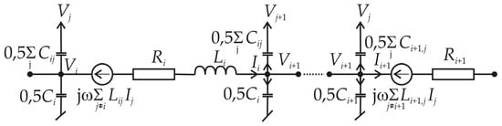
Figure 1.
Π-shape model of the single turn, where Li and Ri are inductance and resistance of i-th turn; Ci is the capacitance of i-th turn to ground; Lij is the mutual inductance between turns i and j; Cij is the capacitance between turns i and j.
For serial-connected windings, this model delivered very good results [8,15]. However, the application of this model for parallel-connected windings resulted in a significant increase of the cross-capacitances, changing the FRA characteristics at high frequencies. For this reason, we used Γ-shape network elements.
The network element shown in Figure 2 corresponds to the single turn of a winding. It allows for inductive and capacitive couplings to all other turns, even if the number of turns is large and the couplings to distant wires do not seem to be significant. The only thing that has been neglected in the network is the resistance to the ground, which, in our experience, does not influence the frequency response. The solution is carried out by a direct algorithm, without using external network simulators.
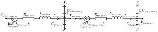
Figure 2.
Single network element with couplings to the next turns.
In Figure 2, the variable M denotes the number of serial turns in one parallel coil; m is the analyzed turn number in the coil; and l is the number of subsequent parallel coil. The subscript j denotes any other turn in the winding. The model of a single turn, shown in Figure 2, consists of self-inductances LM(l − 1)+m, capacitances to the ground CM(l − 1)+m and resistances RM(l − 1)+m, and mutual inductances LM(l − 1)+m, j and capacitances between turns CM(l − 1)+m, j. The adopted model of a Γ-shape is characterized by the fact that it includes the mutual inductances and capacitances between all turns of the winding.
Figure 3 shows the input and output of L-parallel-connected coils. In this case, the total number of turns is equal to N = M·L. The number of the analyzed turn is M(l − 1) + m, with l = 1…L, m = 1…M. A value of m = 1 means the beginning of the winding, while m = M winding’s end. The turns are numbered in such a manner that m = 1…M changes first, and then l = 1…L.
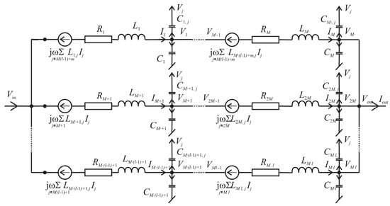
Figure 3.
Input and output elements in the setup of parallel coils, based on the single element from Figure 2.
Other windings of the transformer, existing on the same core, were reduced to a single wire, coupled to all other turns of the analyzed winding, as shown in Figure 4.
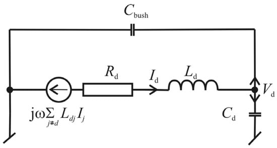
Figure 4.
Additional wire representing other windings of transformer with the bushings’ capacitance.
The additional wire, denoted by subscript d, contains its inductance, resistance, capacitance to the ground, the bushings’ capacitance, and the inductive coupling to other wires. The capacitances to other wires were neglected because the influence of this wire on the FR curve can only be seen for low frequencies.
First, we write L voltage equations for the input elements (m = 1):
Next, we write (M − 1)L voltage equations for the remaining turns:
and its amount is (M − 2)L.
For the output elements, we have one current equation:
where Vout is the output voltage, and R0 is the input resistance of an FR-meter.
For the remaining elements, we can write (M − 1)L current equations:
For the output of the model, there are necessary L equations:
The number of unknown voltages and currents equals the number of equations. Assuming the known excitation Vin = 1, the equations system (1)–(7) provides the solution for the output voltage Vout.
3. Description of the Object and Its Finite Element Model
The simulations were carried out for the active part of an 800 kVA, 15/0.4 kV distribution transformer, which is shown in Figure 4. The left column, which was the object of modelling, has both high-voltage (HV) and low-voltage (LV) windings. In the middle column, only the LV-winding is mounted, so its construction can be seen, and all geometrical measurements are taken. The third column, not shown in the Figure 5, had both windings removed. The active part of the transformer was taken out of the tank and disconnected from the bushings; the measurement was taken directly on the winding leads, to ensure similar conditions to the model. The access to the core, LV winding, and HV winding allowed us to take measurements of the real object geometry. As a consequence, the model was based on the exact dimensions of the transformer, which is often hard to obtain in modelling of oil insulated transformers.
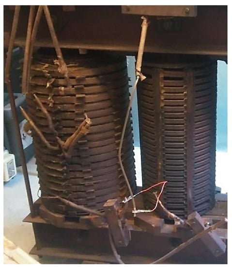
Figure 5.
Windings of the tested active part of the distribution transformer.
The LV-windings of this transformer contain 24 turns connected in 12 parallel branches. Preparation of the 3D finite element model of the winding including 288 separate wires is impractical due to the long computation time in FEM software and is difficult to verify when analyzing several configurations of model parameters. From this reason, the authors used a 2D model. It is obvious that 2D modelling requires a simplification of the real object. Therefore, certain actions should be taken in order to reduce the disadvantages of the 2D model. One of the possible ways is equalization of the core reluctances of the 2D and 3D models. This approach is described in detail in [14] and [15] and is also applied in this case.
Finite element calculations were carried out by utilizing ANSYS Electromagnetic Suite 19.2. The structure of the 2D model is shown in Figure 6.
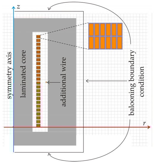
Figure 6.
The 2D model used in finite element calculations.
The same geometry of the model was used both in electrostatic and eddy current calculations. Application of a ballooning boundary condition made it possible to cut off the region of analysis near the core. For the laminated core, the equivalent values of permeability and conductivity were applied. The initial value of the relative magnetic permeability µr was equal to 510, its values for higher frequencies were obtained from the formulas for one-dimensional field penetration into ferromagnetic and conducting material, as described in [24]. The function of the complex permeability is shown in Figure 7. It was calculated for the thickness of the steel sheet of 0.23 mm and equivalent laminated steel conductivity of γ = 1.2 MS/m.
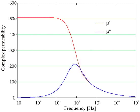
Figure 7.
Complex permeability of laminated core as a function of frequency.
The equivalent electric conductivity of the core was calculated under the assumption that the electromagnetic energy stored in the laminated core equals the energy stored in a monolithic block with equivalent conductivity [24]. This leads to a very simple formula:
where n denotes the number of steel sheets in the core.
4. Obtaining Lumped Parameters
The ANSYS Electromagnetic Suite provides an opportunity to obtain the lumped parameters of the wires, as well as the mutual values for pairs of wires. To calculate the own and mutual capacitances, the electrostatic model is solved for scalar magnetic potential Φ:
and subsequently the capacitances are derived from the electric energy:
For the own and mutual inductances and resistances, the eddy current solver utilizing magnetic vector potential A is as follows:
and the inductances are calculated from the magnetic energy:
while the resistances follow from the power dissipation:
ANSYS allows the obtained values to be exported in the form of matrices. These matrices are directly used in the network model, which is described in Section 2.
5. Simulation Results and Comparison to Frequency Response Measurement
The first test of described algorithm was carried out on a simple air-cored coil, containing 54 turns. Figure 8 presents the comparison of measurement data with the model.
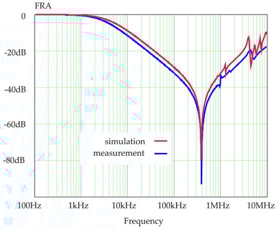
Figure 8.
Test results obtained for air-cored coil with 54 serial connected turns.
This test revealed a good correlation of model with the measurement results up to approximately 5 MHz. Next, the authors proceeded to the tests of transformer windings with a laminated core and parallel connections.
The frequency response of the tested transformer obtained by using the proposed field-network model is compared to the FRA measurement in Figure 9. The FRA measurement was made on the tested winding with an Omicron FRAnalyzer. The test was carried out in an end-to-end open configuration, where the signal was applied at the beginning of the winding and measured at its end. All other windings were left open. The technique and principles of the measurement complied with the recommendations of the IEC standard [1].
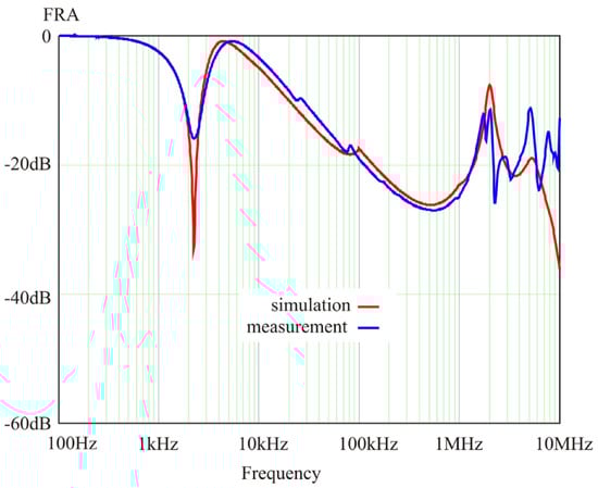
Figure 9.
Frequency response of proposed model compared to measurement.
The conformity of both curves is good up to approximately 3 MHz. This is satisfactory because standard FRA measurements are carried out at up to 2 MHz. In this high frequency range, the frequency response of the winding is strongly influenced by the test configuration, the quality of the connections, and the wave phenomena in the windings. The computer model does not take these effects into account, leading to the visible differences in the frequency response curves of the model and the actual coil above 2 MHz.
The magnitude of the first resonance in the simulation lies much deeper than the first resonance in the real transformer. Moreover, the quality factor is larger than the one from the measurement. The cause of this lies in the simplifications of the assumed model. In the real transformer, each wire of the analyzed winding couples with each wire of the primary winding and its distributed capacitances. In our model, the primary winding is reduced to one turn, and its capacitances are concentrated in Cd. This causes resonance of a larger amplitude and a larger quality factor.
In the next step, a short circuit between two discs, 9 and 10, was introduced into the winding, and the measurement was performed. This location was chosen to be approximately in the middle of the column and without interleaved turns. Only two of the most outer turns were shorted together, which simulates a possible fault in the real transformer (the remaining parallel turns were left undisturbed). It can be seen from Figure 10 that such a local change in the electric circuit strongly influenced the whole frequency range. The first resonance is significantly reduced and shifted into a higher frequency, and the descending slope of the curve is lifted to a smaller damping. Above 1 MHz, the new curve becomes more horizontal than the previous one.
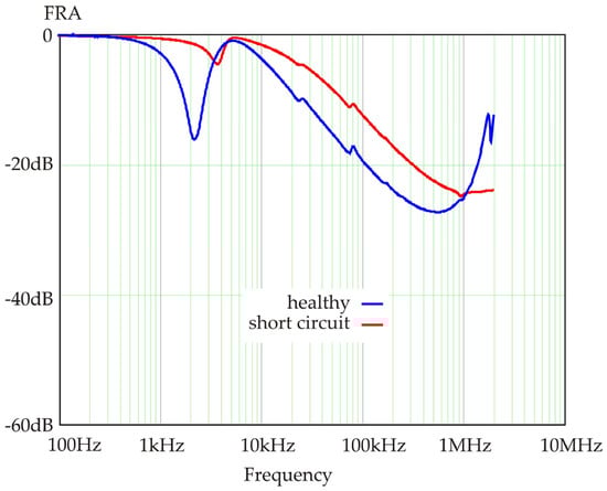
Figure 10.
Frequency response measured on the real winding: blue—healthy winding; red—after introducing the short circuit between discs 9 and 10.
The same defect was simulated in the model by modification of the equations corresponding to the shorted discs. The effect is similar to the measurement, as it can be observed in Figure 11. The first resonance is shifted and reduced, and there are also changes in the damping at higher frequencies. Moreover, the last region, above 1 MHz, changes as in the case of the measurement. The simulation was calculated up to 2 MHz, because that was the limit of the measurement, which was performed according to the standard [1].
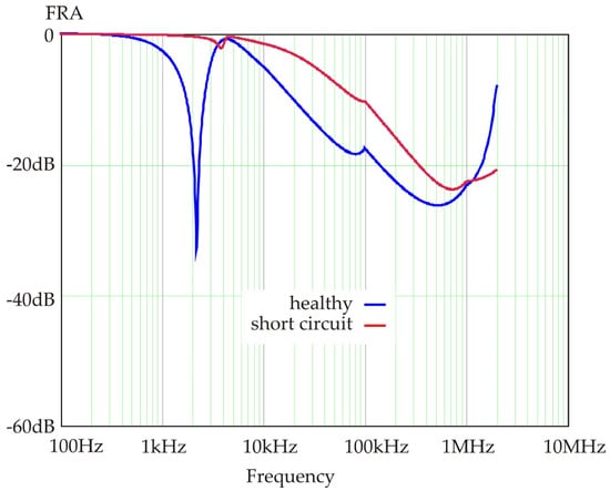
Figure 11.
Frequency response of the model for the healthy case (blue line) and with a simulated short circuit between discs 9 and 10 (red line).
The authors conducted the assessment of measurements and modelling results, presented on Figure 10 and Figure 11, with the most common numerical indices applied in this field in many publications. There are over a dozen of them [26,27], so authors chose four that represent all possible behaviors of such indices, as are proven in the paper [28]. These indices are MSE (Mean Squared Error), CC (Correlation Coefficient), ASLE (Absolute Sum of Logarithmic Error), and SD (Standard Deviation). Their formulas are given below:
The results of the assessment are given in Table 1, both for the measurements and models, where the comparison was performed for different winding status and also between measurements and models. Each value represents the calculations done with given numerical index for two datasets: FRA measurement for the healthy winding and with the short circuit (column 2); the model results for the healthy winding and with the short circuit (column 3); the measurement and the model for the healthy winding (column 4); and the measurement and the model for the winding with the short circuit (column 5).

Table 1.
Results of the assessment with CC, SD, MSE, and ASLE indices.
It can be seen that obtained values are similar in both pairs of analyzed data: when comparing the measurement and the model separately—columns 2 and 3, and when comparing healthy winding results with the short-circuit results—columns 4 and 5. Some larger differences can be seen in column 4, for the comparison of the model results with the FRA measurement for the healthy case results visible on Figure 10 and Figure 11 depth of the parallel resonance at 2 kHz. This assessment with numerical indices proved that the proposed model can be used for the simulation of windings having parallel turns.
6. Conclusions
The research presented in this paper provides a model for the simulation of the frequency response of the active part of a transformer. In order to apply the proposed electromagnetic field/network method, the equivalent values of electric conductivity and magnetic permeability for the laminated core should first be established for a wide frequency range. Then, the finite elements model, taking into account the proper core parameters, allows the calculation of the lumped parameters, R, L, and C, of the winding. The obtained parameters are applied to the network algorithm, which considers the winding connection method. In the paper, the algorithm for windings connected in parallel was developed.
The obtained results allow for the simulation of the frequency response curves for various winding distortions and faults. Frequency response analysis is one of the standard diagnostic methods for transformer diagnostics, but its applicability is limited by difficulties in the interpretation of the results. The biggest problem is linking the changes in measured FR signatures with the actual mechanical condition of the active part of the transformer. Therefore, the frequency response simulations of the various winding conditions using models utilizing the electromagnetic field and an RLC network could improve the efficiency of the assessment of winding faults by the FRA method. The proposed approach is able to simulate faults in the winding, which was presented by using the example of a short circuit between two adjacent discs and assessed with four the most typical numerical indices used in the FRA diagnostics. By providing modifications in corresponding equations, it is possible to simulate the influence of this fault, which is similar to data obtained from the measurement.
Author Contributions
Conceptualization, S.B., K.M.G. and K.T.; Methodology, K.G., S.B. and K.T.; Software, K.M.G. and K.T.; Validation, K.M.G. and K.T.; Formal Analysis, S.B. and K.M.G.; Investigation, S.B., K.M.G. and K.T.; Resources, K.M.G. and S.B.; Writing Original Draft Preparation, K.M.G., S.B. and K.T.; Writing Review & Editing, S.B. and K.M.G.; Visualization, K.M.G., S.B. and K.T.; Supervision, S.B. and K.M.G.; Project Administration, S.B. All authors have read and agreed to the published version of the manuscript.
Funding
This research received no external funding.
Conflicts of Interest
The authors declare no conflict of interest.
References
- IEC. IEC 60076-18: Power Transformers—Part 18: Measurement of Frequency Response; IEC Standard: Geneve, Swietzerland, 2012. [Google Scholar]
- IEEE. IEEE Guide for the Application and Interpretation of Frequency Response Analysis for Oil-Immersed Transformers; IEEE Std C57.149-2012: Piscataway, NJ, USA, 2013. [Google Scholar]
- Bagheri, M.; Nezhivenko, S.; Phung, B.T.; Behjat, V. On-load Tap-changer Influence on Frequency Response Analysis of Transformer: A Case Study. In Proceedings of the 11th Int. Symposium on Diagnostics for Electrical Machines, Power Electronics and Drives, Tinos, Greece, 29 August–1 September 2017. [Google Scholar]
- Banaszak, S.; Szoka, W. Influence of a tap changer position on the transformer’s frequency response. In Proceedings of the 2018 Innovative Materials and Technologies in Electrical Engineering (i-MITEL) Conference, Sulecin, Poland, 18–20 April 2018; pp. 1–4. [Google Scholar]
- Sofian, D.M.; Wang, Z.D.; Li, J. Interpretation of Transformer FRA Responses—Part II: Influence of Transformer Structure. IEEE Trans. Power Deliv. 2010, 25, 2582–2589. [Google Scholar] [CrossRef]
- Abu-Siada, A.; Hashemnia, N.; Islam, S.; Masoum, M.A.S. Understanding Power Transformer Frequency Response Analysis Signatures. IEEE Electr. Insul. Mag. 2013, 29, 48–56. [Google Scholar] [CrossRef]
- Senobari, R.K.; Sadeh, J.; Borsi, H. Frequency response analysis (FRA) of transformers as a tool for fault detection and location: A review. Electr. Power Syst. Res. 2018, 155, 172–183. [Google Scholar] [CrossRef]
- Banaszak, S.; Gawrylczyk, K.M.; Trela, K.; Bohatyrewicz, P. The Influence of Capacitance and Inductance Changes on Frequency Response of Transformer Windings. Appl. Sci. 2019, 9, 1024. [Google Scholar] [CrossRef]
- Tenbohlen, S.; Coenen, S.; Djamali, M.; Müller, A.; Samimi, M.H.; Siegel, M. Diagnostic Measurements for Power Transformers. Energies 2016, 9, 347. [Google Scholar] [CrossRef]
- Alsuhaibani, S.; Khan, Y.; Beroual, A.; Malik, N.H. A Review of Frequency Response Analysis Methods for Power Transformer Diagnostics. Energies 2016, 9, 879. [Google Scholar] [CrossRef]
- Abeywickrama, N.; Serdyuk, Y.V.; Gubanski, S.M. Effect of Core Magnetization on Frequency Response Analysis (FRA) of Power Transformers. IEEE Trans. Power Deliv. 2008, 23, 1432–1438. [Google Scholar] [CrossRef]
- Azzouz, Z.; Foggia, A.; Pierrat, L.; Meunier, G. 3d Finite Element Computation of the High Frequency Parameter of Power Transformer Windings. IEEE Trans. Magn. 1993, 29, 1407–1410. [Google Scholar] [CrossRef]
- Mitchell, S.D.; Welsh, J.S. Modeling Power Transformers to Support the Interpretation of Frequency-Response Analysis. IEEE Trans. Power Deliv. 2011, 26, 2705–2717. [Google Scholar] [CrossRef]
- Bjerkan, E. High Frequency Modeling of Power Transformers. Stresses and Diagnostics. Ph.D. Thesis, Norwegian University of Science and Technology, Trondheim, Norway, 2005. [Google Scholar]
- Gawrylczyk, K.M.; Banaszak, S. Computer Modeling in the Diagnostics of Transformers’ Windings Deformations. Comput. Appl. Electr. Eng. 2010, 8, 132–140. [Google Scholar]
- Florkowski, M.; Furgał, J. Modelling of winding failures identification using the Frequency Response Analysis (FRA) method. Electr. Power Syst. Res. 2009, 79, 1069–1075. [Google Scholar] [CrossRef]
- Zhao, X.; Yao, C.; Abu-Siada, A.; Liao, R. High frequency electric circuit modeling for transformed frequency response analysis studies. Int. J. Electr. Power Energy Syst. 2019, 111, 351–368. [Google Scholar] [CrossRef]
- Abeywickrama, N.; Serdyuk, Y.V.; Gubanski, S.M. High frequency modelling of power transformers for use in frequency response analysis (FRA). IEEE Trans. Power Deliv. 2008, 23, 2042–2049. [Google Scholar] [CrossRef]
- Al-Ameri, S.; Yousof, M.F.M.; Aziz, N.; Avinash, S.; Talib, M.A.; Salem, A.A. Modeling frequency response of transformer winding to investigate the influence of RLC. Indones. J. Electr. Eng. Comput. Sci. 2019, 14, 219–229. [Google Scholar] [CrossRef]
- Murthy, A.S.; Azis, N.; Al-Ameri, S.; Yousof, M.F.M.; Jasni, J.; Talib, M. Investigation of the effect of winding clamping structure on Frequency Response Signature of 11 kV distribution transformer. Energies 2018, 11, 2307. [Google Scholar] [CrossRef]
- Hashemnia, N.; Abu-Siada, A.; Masoum, M.A.S.; Islam, S. Characterization of Transformer FRA Signature under Various Winding Faults. In Proceedings of the Condition Monitoring and Diagnosis Conference, Bali, Indonesia, 23–27 September 2012. [Google Scholar]
- Dick, E.P.; Erven, C.C. Transformer Diagnostic Testing by Frequency Response Analysis. IEEE Trans. Power Appar. Syst. 1978, PAS-97, 2144–2153. [Google Scholar]
- Eslamian, M.; Vahidi, B. New Methods for Computation of the Inductance Matrix of Transformer Windings for Very Fast Transients Studies. IEEE Trans. Power Deliv. 2012, 27, 2326–2333. [Google Scholar] [CrossRef]
- Gawrylczyk, K.M.; Trela, K. Frequency Response Modeling of Transformer Windings Utilizing the Equivalent Parameters of a Laminated Core. Energies 2019, 12, 2371. [Google Scholar] [CrossRef]
- Liu, S.; Liu, Y.; Li, H.; Lin, F. Diagnosis of transformer winding faults based on FEM simulation and on-site experiments. IEEE Trans. Dielectr. Electr. Insul. 2016, 23, 3752–3760. [Google Scholar] [CrossRef]
- Rahimpour, E.; Jabbari, M.; Tenbohlen, S. Mathematical comparison methods to assess transfer functions of transformers to detect different types of mechanical faults. IEEE Trans. Power Deliv. 2010, 25, 2544–2555. [Google Scholar] [CrossRef]
- Badgujar, K.P.; Maoyafikuddin, M.; Kulkarni, S.V. Alternative statistical techniques for aiding SFRA diagnostics in transformers. IET Gener. Transm. Distrib. 2012, 6, 189–198. [Google Scholar] [CrossRef]
- Banaszak, S.; Szoka, W. Transformer frequency response analysis with the grouped indices method in end-to-end and capacitive inter-winding measurement configurations. IEEE Trans. Power Deliv. 2019. [Google Scholar] [CrossRef]


© 2020 by the authors. Licensee MDPI, Basel, Switzerland. This article is an open access article distributed under the terms and conditions of the Creative Commons Attribution (CC BY) license (http://creativecommons.org/licenses/by/4.0/).