Abstract
The electric rudder system (ERS) is the executive mechanism of the flight control system, which can make the missile complete the route correction according to the control command. The performance and quality of the ERS directly determine the dynamic quality of the flight control system. However, the transient and static characteristic of ERS is affected by the uncertainty of physical parameters caused by nonlinear factors. Therefore, the control strategy based on genetic algorithm (GA) identification method and finite-time rudder control (FTRC) theory is studied to improve the control accuracy and speed of the system. Differently from the existing methods, in this method, the difficulty of parameter uncertainty in the controller design is solved based on the ERS mathematical model parameter identification strategy. Besides, in this way, the performance of the FTRC controller was verified by cosimulation experiments based on automatic dynamic analysis of mechanical systems (ADAMS) (MSC software, Los Angeles, CA, USA) and matrix laboratory (MATLAB)/Simulink (MathWorks, Natick, MA, USA). In addition, the advantages of the proposed method are verified by comparing with the existing strategy results on the rudder test platform, indicating that the control accuracy is improved by 70% and the steady-state error is reduced by at least 50%.
1. Introduction
The electric rudder system (ERS) is the position servo mechanism of high-precision control systems such as aircraft, ship, and missile, whose dynamic and static performance directly determines the accuracy and rapidity of the controlled object [1]. Compared with hydraulic rudders and pneumatic rudders, electric rudders are simple, reliable, low-cost, and high-precision. Hence, obtaining a high-efficiency ERS controller is a very practical and meaningful study. The structure of an ERS is shown in Figure 1, which is mainly composed of a motor, a screw, a reduction, and a rocker arm. In order to overcome the interference of different nonlinear factors in the design of the controller based on the ERS parameter model, research has made a lot of efforts from two aspects.
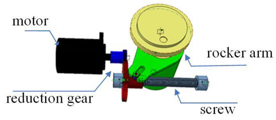
Figure 1.
Schematic diagram of an electric rudder system.
On the one hand, the accuracy of the actual physical parameters of the ERS is ensured by using identification techniques. In the past, optimization methods for parameter identification were generally divided into classic algorithms and intelligent algorithms. The least-square method in the classical algorithm is the most widely used identification method. Its optimization principle is to continuously optimize unknown parameters by minimizing the sum of the squared errors of the identification output and the actual output [2,3]. One such method is proposed in [4] for parameter identification in ERS models. However, classical optimization algorithms often face the problems of local optimization and slow convergence speed. Compared with traditional algorithms, intelligent optimization algorithms have higher efficiency and reliability in dealing with practical complex and changeable optimization problems [5,6,7]. Intelligent optimization algorithms are usually inspired by physical phenomena of real intelligent biology, and genetic algorithm is widely used because of its simple process, strong scalability, and fast search ability unrelated to the problem field. In [8], the genetic algorithm is applied to the ERS parameter identification experiment, and the improved algorithm is proved to have good optimization effect by comparing with the classical optimization algorithm such as the least square method. Therefore, the genetic algorithm (GA) has the advantage of not needing to know the prior conditions such as the system structure, so it is suitable for parameter identification of ERS.
On the other hand, the influence of uncertain factors can be solved by designing special control methods. In [9], the classical proportional integral differential (PID) control method is studied, and the experimental results show the superiority of the algorithm control performance. However, when the ERS encounters various parameter changes and nonlinearities during dynamic high-speed motion, it cannot ensure acceptable tracking performance. Robust sliding mode control is also applied to controller design due to its strong robustness to system uncertainties [10,11]. For example, in [10], a robust adaptive sliding mode controller is proposed for ERS, which uses the ability of adaptive online estimation to estimate the boundary of uncertain parameters and the adjustable gain of the sliding mode controller. Nevertheless, the parameters of the process update are greatly affected when the nonlinearity of the system is large. Fuzzy control does not require the accurate mathematical model of the controlled object and is applied to the design of the ERS controller [12], which achieves a good tracking performance of the system. However, how to obtain fuzzy rules and membership functions is completely based on experience. In addition, adaptive technology is also widely used in the design of controllers due to the low requirements for the precise model of the controlled object [13,14]. In [15], because the process parameters are adaptively updated and applied to the ERS system, the initial parameter requirements of the controller design are not very demanding. However, if there is a large parameter uncertainty, it will lead to inaccurate system identification and affect system performance.
The analysis of the above control methods shows that the exponential convergence form based on Lyapunov asymptotic stability is the fastest. However, these control analyses are based on Lipschitz continuous infinite stable control methods. Fortunately, finite-time control has been widely used in control theory and applied research due to its advantages in convergence speed and convergence accuracy. In reference [16], the finite-time theoretical controller of linear parameter time-varying system and linear time-delay system is designed, and the effectiveness of the method is proved by the servo mechanism experiment. In [17], the theoretical idea of combining adaptive and finite-time theory is proposed. The advantage of fast convergence in finite time is used to improve the convergence speed of adaptive estimation, and the ability of the system to adapt to change is further improved. As far as we know, the method of combining the identification technology with the finite-time control theory to better design the controller is scarce but very valuable. In [18], the finite-time servo control technology and particle swarm optimization (PSO) algorithm identification technology were combined to design a more accurate and effective ERS controller. The experimental results show the effectiveness of the finite-time control method based on the identification model.
Inspired by parameter identification and special control methods to solve uncertain parameters in ERS controller design, in this paper, firstly, ERS parameter identification algorithm uses linear ordering to perform selection operations, nonlinear uniform crossover operators, Gaussian mutation operators, and adaptive crossover and mutation probabilities. Then, the finite-time control theory is studied and its stability is proved. Finally, the finite-time controller is designed by applying the improved genetic algorithm (IGA) to the system model parameter identification. This paper is organized as follows. The dynamic characteristics model of ERS is described in Section 2 for subsequent model parameter identification and controller design. In Section 3, an improved genetic algorithm and a finite-time control strategy are introduced. Then, the simulation experiments are compared with the existing control strategies to verify the effectiveness of the finite-time rudder control (FTRC) strategy based on IGA identification in Section 4. In Section 5, the ERS experimental platform is introduced, and the effectiveness of identification strategy and control method is verified by experiments. Finally, Section 6 gives the conclusion of the study.
2. Model of Electric Rudder System
2.1. System Description
Figure 2 shows the structure of the ERS and the principle of information transmission process. Its structure includes controller, rudder, motor, gearbox, feedback potentiometer, and return spring rudder surface. The function of the ERS is to control the attitude and trajectory by driving the rudder surface after receiving the command signal from the control system. Its output is a closed-loop control system of displacement (angle), velocity, or acceleration, and its role is to enable the output to accurately track the input. The controller is a unit that performs arithmetic processing on the servo control system and converts the received control signals into corresponding driving currents to control the motor. The servo motor receives the controller’s electrical signal and converts it into the corresponding speed and torque output. Meanwhile, the position information feedbacks to the drive controller through the encoder, so that the system forms a closed loop. Therefore, with the widespread application of servo control systems and the rapid development of related technologies, it is of great significance to perform efficient and reliable control of servo control systems.
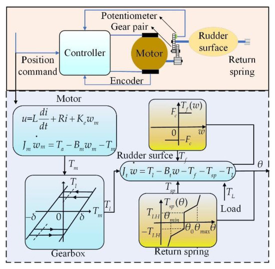
Figure 2.
Block diagram of the electric rudder system and information transmission process.
Considering the nonlinear characteristics such as friction and torque connection between the motor and the rudder surface, the dynamic model of the ERS is described by the equation of motion of the linear DC motor and the rudder surface. System dynamics can be described as:
where u is the control voltage signal, ia is the armature current, wm is the motor angular velocity, and θ and w are the output angle and angular velocity of the ERS, respectively. R and L are the resistance and inductance, respectively. Ke and Kt are the back electromotive force constant and the torque constant, respectively. Jm, Bm and Jt, Bt are the moment inertia and viscous damping constant of the motor and rudder axle, respectively. TL is the load torque, and Tsp and Tf are return spring torque and friction torque, respectively, as follows:
where θ0 is the initial angle of the ERS, TLH and ks are the offset and gain, respectively, and Tm and Tl are the input and the output torque of the gearbox, respectively. The backlash nonlinearity is usually described by
where n is the gear ratio, δ is the backlash distance, and Tl(t_) means that no change occurs in Tl(t). When the armature inductance L is very small, the armature hysteresis effect is ignored. Therefore, in the controller design, the equivalent second-order system state space of the ERS dynamic equation is as follows:
where J = Jt + n2Jm and B = Bt + n2Bm are the equivalent total inertia and viscous damping constant, respectively. In actual work, the physical parameters L, R, ks, TLH, Fc, J, B, Kt, Ke, and n are greatly affected by nonlinear factors. Further defining , , , , turns the control-oriented model (5) into the following form:
Therefore, in order not to be affected by nonlinear factors, the research direction is usually from two aspects: system parameter identification and special control method. Since the armature inductance value L is small, the armature current dynamics ia in Equation (1) can be neglected, so it can be considered as u = Kewm. Kewm is the back electromotive force (EMF) generated by the permanent magnet in the armature of the motor. Note that the use of an integrator to obtain zero steady-state error is applicable to a constant reference signal. According to the internal model principle, the tracking error integral is extended to the state variable, and the control-oriented system model is described as:
where , , , is the reference input, , , a3 = a1θ0, , , , , .
2.2. Fundamental Lemma
The related lemma of finite-time control is introduced below to pave the way for the theoretical research of finite time.
Lemma 1
[19]. For any real number xi, i = 1, …, n, x, y and 0 < q ≤ 1. The following inequality holds
when 0 < q = q1/q2 ≤ 1. The following inequality holds
where q1 and q2 are odd integers.
Lemma 2
[19]. For any real numbers c, d > 0 and real-valued function γ(x, y) > 0
Lemma 3
[19]. Assume the following non-Lipschitz continuous system
Suppose there exists a continuous function V: such that the following conditions hold:
- (1)
- V: .
- (2)
- There exist real numbers c > 0, a∈(0,1) and an open neighborhood containing the origin, so that the following conditions are true
For system (11), it is finite-time stable if it is Lyapunov stable in neighborhood , and its state can converge to equilibrium point x = 0 within a finite time. A more precise description is that if there is a function T(x0): U\{0}→(0,∞), so that for , the system is decoded as x(t, x0). For x(t, x0)∈U\{0} and , when t∈[0, T(x0)], for t > T(x0), there is x(t, x0) = 0, then the system is stable for local finite time. On the basis of this, if , the system is global finite-time stable.
3. Strategy Based on GA Identification
3.1. GA-Based Parameter Identification
Genetic algorithm (GA) is an intelligent optimization algorithm based on the principles of natural selection and genetics. It is an efficient optimization method that seeks the global optimal solution without any initialization information [20]. In GA, each individual represents a separate solution. By ranking the fitness value of each solution to determine the quality of each iteration optimization. We can find the best solution by simulating the crossover and mutation of organisms in nature. The identification diagram is shown in Figure 3. The fitness function uses the integral square error (ISE) criterion of the following formula:
where θa refers to the output angle of the ERS after responding to the control command, that is, the actual output angle collected by the test system. θi refers to the output angle after inputting the same control signal to the identification model.
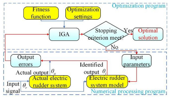
Figure 3.
Identification schematic.
3.2. Improvement on GA
This paper uses GA to identify model parameters because it has strong global search capabilities without prior knowledge. However, as a general random search algorithm, GA still has the defects of premature convergence and slow convergence speed when solving some complex problems. In order to improve the convergence speed and identification accuracy, some measures have been taken in the design of genetic algorithms.
3.2.1. Genetic Operators
The model parameters can be easily encoded on the chromosome via real-number encoding. This chromosome can then be represented by a nine-dimensional array of 9 real-number variables as follows X = [L, R, ks, TLH, Fc, J, B, nKt, nKe]T. The parents are assumed to be Xt = [x11, x12,…, x1n]T, and any offspring to be X t + 1. The selection operation uses a linear sort selection method, and its selection probability is:
where m is the population number, j is the index number in descending order, η− and η+ are the worst and best individual expected values of the individual, respectively, and their relationship is η+ + η− = 2.
The purpose of cross-operation is to expand the range of population search, so as to ensure the diversity of population individuals. In order to avoid the tedious encoding and decoding process of binary encoding, we use the arithmetic crossover operator commonly used in real encoding. Meanwhile, nonuniform linear crossings are introduced. Assuming the parents are and , the offspring resulting from the crossover process are:
where c is a scale factor randomly generated between (0, 1).
In order to make the algorithm converge quickly and suppress the premature convergence of the population, the following modified mutation operator is used. The mutation operator uses the Gaussian mutation method as follows:
where N(0, σ) is Gaussian distribution and σ is variance. In order to speed up convergence, σ is set as a variable parameter in this paper
where t and G are the current and total evolutionary generations, respectively.
3.2.2. Adaptive Crossover and Mutation Probability
Because the cross probability Pc and mutation probability Pm play a key role in the optimization characteristics of GA, the fixed probability cannot meet the overall characteristics. The cross and mutation probability values of traditional GA are usually set according to specific situations. Therefore, there is a great blindness in setting the specific value. The larger the cross probability Pc, the easier the genetic model will be destroyed, and the slower the optimization speed will be if the Pc is too small; the smaller the mutation probability Pm is, the lower the probability of generating new individuals will be, and the GA will become a blind random search algorithm if the Pm is too large. In order to find the best value of each problem, adaptive cross probability and mutation probability methods are applied. The sigmoid function is introduced to obtain the probability of adaptive crossover and mutation.
where Pc1 and Pc2 are the initial cross probability and the final cross probability, respectively. Pm1 and Pm2 are the initial mutation probability and the final mutation probability respectively. Ns is the cutoff point, being set to 0.25, and α is the shape factor, being set to 20. G is the total generation. The flowchart of the improved genetic algorithm is shown in Figure 4.
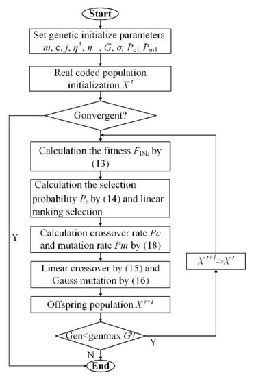
Figure 4.
Flowchart of the improved genetic algorithm.
3.3. Controller Based on Finite Time
The adaptive backstepping recurrence technique is introduced into the framework of finite-time stability theory, and the control law and adaptive law are obtained.
Step 1: For the subsystem x1 of (7), a virtual control law renders the derivative of to satisfy
where k1 > 0 is an adjustable parameter, q = q1/q2∈(2/3,1).
Step 2: For the subsystem (x1, x2), the time derivative of is calculated as:
where .
Applying Lemmas 1 and 2 to the first term and the last term of the second inequality of (19), it follows
Then, substituting (21) into (20) yields
Again applying Lemma 2, , and defining the virtual control law , (22) becomes
where γ1, γ2, k2 are adjustable positive parameters.
Step 3: For the system (7) with a positive definite function
The time derivative of V3(x1, x2, x3) satisfies
where 0 < l < 1, .
Moreover, considering (23), by Lemmas 1 and 2
where γi > 0,(i = 3, 4, …, 7) are adjustable parameters, and
and considering (8)–(9), the following inequality holds
Therefore, a control law designed as the form
where k3 > 0 is an adjustable parameter. Then, substituting (23), (26), (27), and (28) into (25), and considering the system (7) and the definitions of and m1, m2, m3 of (33)–(35), satisfies the following formulas:
where
Meanwhile, by Lemma 1 V3(x1, x2, x3) satisfies
Then, by Lemma 1, the following inequality holds.
where . From the above description and Lemma 3, it is concluded from (24) and (37) that the system (7) is stable to in the finite time of equilibrium point x = 0. In short, the proposed control strategy (31) ensures that the system (6) has the required angle of higher static performance in a limited time.
In order to make the parameter selection of the controller design in this paper have basis, the paper gives the guidance of the controller adjustable parameter selection:
- (1)
- q is chosen as a fraction satisfying q ∈ (2/3, 1) with the odd numerator and denominator; generally, it may be more likely to close to 1.
- (2)
- This paper chooses L ∈ (0, 1) by determining (32), so as to reduce the influence of uncertain parameters on the convergence rate. Therefore, on the premise of satisfying the convergence rate, the parameter should be as small as possible.
- (3)
- The choice of k1, k2, and k3 is mainly based on guaranteeing the positiveness of m1, m2, and m3; that is, inequality (33)–(35) holds. Note the interrelations and constraints between k1, k2, and k3 in (33)–(35). Their selection follows the following guidelines: first, k1 is selected by guaranteeing inequality (33). Then, choose k2 to be greater than k1 according to (34). After that, select k3 to be greater than k1 and k2 according to (35). It should be noted that a larger k3 will increase the burden on the control input u from (31).
- (4)
- γi (i = 1, …, 7) are just for guaranteeing the positiveness of m1, m2, and m3.
The control strategies proposed in this paper are summarized as follows: First, the ERS model parameters are identified through IGA to pave the way for controller design. Then, the finite-time stability of the ERS system is designed using finite-time stability with faster convergence speed than asymptotic stability. Finally, the stability of the closed-loop system is analyzed.
4. Simulation Comparison with Existing Strategies
In this section, the method of cosimulation experiments was used to verify the comparison between the control method in this paper and the existing control strategies. Automatic dynamic analysis of mechanical systems (ADAMS) was used to construct the ERS mechanical dynamics model, and matrix laboratory (MATLAB)/Simulink environment was used to verify the controller. As shown in Figure 5 and Figure 6, in order to realize the cosimulation of the following system based on ADAMS and MATLAB/Simulink, the setting steps are as follows: First, determine the state variable of the mechanical virtual prototype model of the follower system. Then, ADAMS/Control is used to determine the model output of the angular velocity input variable and the feedback angular velocity variable of the MATLAB/Simulink follow-up drive system. Finally, the control algorithm proposed in this paper is verified in the MATLAB/Simulink simulation environment. This paper is compared with existing control strategies in this environment.
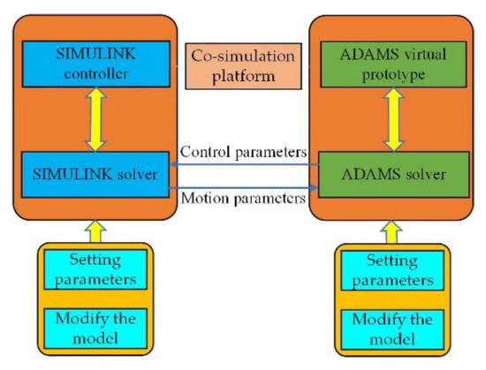
Figure 5.
The scheme of cosimulation.
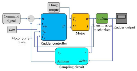
Figure 6.
The scheme of matrix laboratory (MATLAB)/Simulink.
In order to illustrate the effectiveness of the method more intuitively, the classic PID control in [9] and the H∞ control in [21] are given as follows:
where .
In [10], the robust adaptive PID sliding mode control (RASM) strategy, the PID controller in [9], and the H∞ controller in [21] are used to verify the transient performance and robustness. The parameter values constructed by the joint simulation model are shown in Table 1. The simulation experimental system model is the same as that in [10]:

Table 1.
Physical parameter of electric rudder system.
m1 = 0.0075, m2 = 5.7594, m3 = 0.00034.
As shown in Figure 7 and Figure 8, compared with the existing control strategy of ERS, the FTRC control strategy in this paper has better control accuracy and speed.
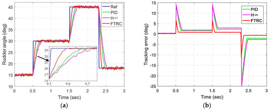
Figure 7.
System response and error of different algorithms under input step signal: (a) system response; (b) system response error.
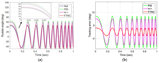
Figure 8.
System response and error of different algorithms under chirp signal: (a) system response; (b) system response error.
5. Experimental Application and Results Analysis
Figure 9 shows the hardware schematic of the ERS test platform to verify the effectiveness and practicability of the proposed FTRC strategy. Firstly, configure the parameters of the controller through Copley Controls CME 2 software, and then send the control signal to the controller through the multifunctional data acquisition card (DAQ) USB-3500. After the controller drives the ERS, the USB-3500 data acquisition card collects the position information feedback by the potentiometer of the servo system. In order to verify the effectiveness of the FTRC proposed in this paper, the paper uses a control strategy based on model parameter identification in practical applications. The experiment is divided into two parts: one is to use IGA to identify ERS parameters and compare the performance with the existing optimization algorithm; the other is to use the identified parameter model in FTRC design and compare it with the existing PID and H∞ control.
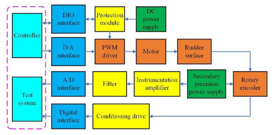
Figure 9.
Electric rudder system test platform.
5.1. Parameter Identification Algorithm Verification
In order to verify the superiority of the proposed IGA optimization performance, a comparative experiment was set up as follows: Firstly, the controller sends the control command (desired angle θr) and collects the feedback signal (actual angle θa). Then, the data is input into the preset model under MATLAB programming to obtain the identification angle θi, and the fitness value is obtained by Equation (13). The function continually updates the model parameters so that θa and θi are constantly approaching. Finally, this paper compares the PSO and GA1 optimization algorithm with IGA. We only compare the number of iteration steps and the size of the fitness value to illustrate. For fair comparison, among the three algorithms, GA1 does not apply adaptive selection and mutation probability, and the rest of the operations are performed according to this article. In this study, parameter error (EPE) and average parameter error (EAPE) were used to evaluate the parameter identification accuracy. The calculation of EPE and EAPE is as follows:
where Xi and are the parameters of the actual system and the identification system, respectively, and D is the dimension of Xi.
Figure 10 shows the change process of fitness values of different optimization algorithms. Compared with other algorithms, the IGA proposed in this paper has fewer iterative steps and can achieve smaller fitness values. In addition, it can be seen from Table 2 that the maximum EPE value of IGA is 20%, which is far less than 48.3% of GA and 47% of PSO, which indicates that the modified mutation and crossover probability and operator operation of this paper can effectively improve the convergence precision and speed.
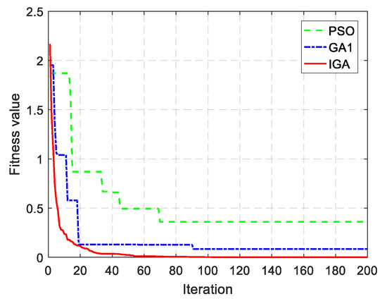
Figure 10.
Parameter identification process.
Table 2.
Electric rudder system identification results.
5.2. Controller Verification
The controller is designed to verify the effectiveness of the control algorithm based on the parameters obtained from the above identification algorithm. Since the actual system physical parameters are different from those of the joint simulation experimental model, the parameters of the controller (31) are set as follows:
The following different laboratory conditions were set up in this paper:
Case 1. The square wave signal is used to verify the transient performance of the FTRC, as shown in Figure 11a.
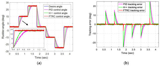
Figure 11.
Actual response and error of different algorithm under input step signal: (a) system response; (b) system response error.
Case 2. The ramp wave signal is used to verify the steady state performance of the FTRC at constant acceleration, as shown in Figure 12a.
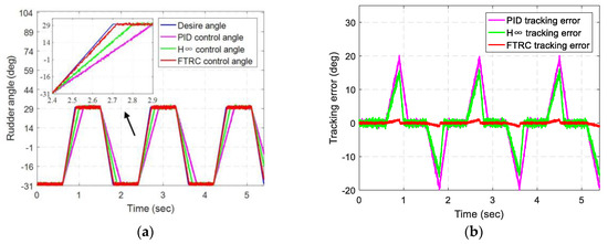
Figure 12.
Actual response and error of different algorithm under input step signal: (a) system response; (b) system response error.
Case 3. The chirp signal from 1 Hz to 20 Hz is used to verify the dynamic performance of the FTRC, as shown in Figure 13a.
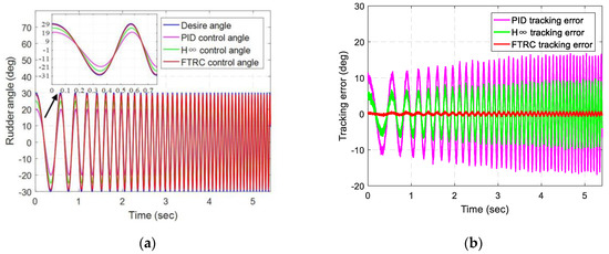
Figure 13.
Actual response and error of different algorithm under input chirp signal: (a) system response; (b) system response error.
The experiment responses of ERS with PID, H∞, and FTRC in the above three cases are shown in the Figure 11a, Figure 12a and Figure 13a, respectively. As can be seen from Figure 11b, Figure 12b and Figure 13b, compared with other methods using the FTRC algorithm in this paper, the tracking accuracy and response speed of ERS have been greatly improved under the same control instructions. Compared with other algorithms, the tracking accuracy is reduced by at least 70%, which proves that the dynamic performance of the control algorithm for ERS has been greatly improved.
In addition, this paper aims to verify the advantages of FTRC control strategies in terms of energy consumption. Figure 14 shows the energy consumption comparison diagram of ERS under Case 1. Therefore, compared with the other two algorithms, the energy consumption of this method is relatively small, which shows that the energy consumption of this method is small.
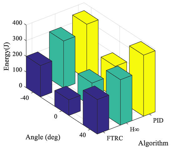
Figure 14.
Bar graphic visualization of the energy consumption performance under Case 1.
Figure 15a,b compares the dynamic and static performance response results of Cases 1 and 2, including the set time (ST), the overshoot (OS), and the steady-state error (SSE). Compared with other methods, it can be seen that the ST of ERS during deceleration and acceleration is within 100 ms, the OS is less than 3%, and the SSE is reduced by at least 50%. Therefore, the effectiveness of the proposed FTRC is illustrated.
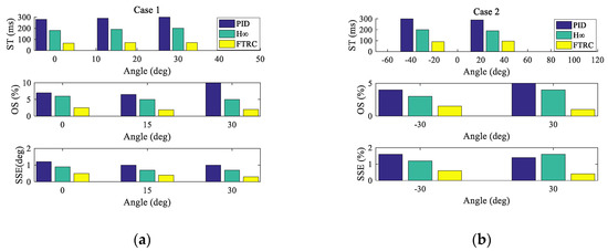
Figure 15.
Setting time, overshoot and steady state error under Cases 1 and 2.
6. Conclusions
In order to improve the control accuracy and speed of ERS and avoid the influence of nonlinear factors, this paper presents a new control method based on genetic algorithm and finite time theory. The crossover operator of the GA uses a nonuniform linear crossover method, and the mutation operator uses a Gaussian mutation method to obtain elite individuals and adaptive mutation and crossover probability based on evolutionary characteristics. A finite time servo controller based on GA identification parameters is designed for ERS, whose convergence rate is faster than the asymptotic stability. The joint simulation experiments verify that it has faster convergence accuracy and convergence speed than the existing control strategies PID and H∞. The efficiency of different intelligent optimization algorithms and the IGA identification parameters proposed in this paper are compared, which proves that the optimization accuracy of the improved optimization algorithm has been greatly improved. In addition, the dynamic and static performance of ERS under different actual conditions was verified on the ERS test bench, which proves the effectiveness of the method proposed in this paper. However, the proposed method has some limitations, such as online identification of ERS parameters in a dynamic and fast environment, and needs further study.
Author Contributions
All authors were involved in the study in this manuscript. Z.W. provided ideas, wrote the paper and conducted the experiment; R.Y. and C.G. provided the theory guidance and instruction; S.G. confirmed the theory; X.C. and Z.W. wrote software programs. All authors have read and agreed to the published version of the manuscript.
Funding
This research was supported in part by International S&T Cooperation Program of China (NO 2014DFR70650), in part by the Fund for Shanxi Province Industrial Project of China under Grant 201703D1210282 and Grant 201803D121058, and in part by the Fund for Shanxi “1331 Project” Key Subject Construction.
Conflicts of Interest
The authors declare no conflict of interest.
References
- Chang, J. Test Method and Model Identification of Flight Control Actuator Based on Video Acquisition. Master′s Thesis, Beijing Institute of Technology, Beijing, China, 2016. [Google Scholar]
- Shi, Z.; Wang, Z.; Ji, Z. A multi-Innovation recursive least squares algorithm with a forgetting factor for Hammerstein CAR systems with backlash. Circuits Syst. Signal Process. 2016, 35, 4271–4289. [Google Scholar] [CrossRef]
- Claes, M.; Graham, M. Frequency domain subspace identification of a tape servo system. Microsyst. Technol. 2007, 13, 1439–1447. [Google Scholar] [CrossRef]
- Liu, G.; Shen, G. Experimental evaluation of the parameter-Based closed-Loop transfer function identification for electro-Hydraulic servo systems. Adv. Mech. Eng. 2017, 9, 1–14. [Google Scholar] [CrossRef]
- Thomas, G.; Lingai, L.; Dominique. Identification of optimal parameters for a small-Scale compressed-Air energy storage system using real coded genetic algorithm. Energies 2019, 12, 377–408. [Google Scholar]
- Liu, H.; Lin, Z.; Xu, Y. Coverage uniformity with improved genetic simulated annealing algorithm for indoor Visible Light Communications. Opt. Commun. 2019, 439, 156–163. [Google Scholar] [CrossRef]
- Liao, J.; Luo, F.; Luo, Z. The parameter identification method of steam turbine nonlinear servo system based on artificial neural network. J. Braz. Soc. Mech. Sci. Eng. 2018, 40, 1–10. [Google Scholar] [CrossRef]
- Wang, J. Research on Parameter Optimization Method of Electric Rudder System. Master′s Thesis, North University of China, Taiyuan, China, 2016. [Google Scholar]
- Deur, J.; Pavkovic, D.; Peric, C. An electronic throttle control strategy including compensation of friction and limp-Home effects. IEEE Trans. Ind. Appl. 2003, 40, 821–834. [Google Scholar] [CrossRef]
- Wang, H.; Liu, L.; He, P. Robust adaptive position control of automotive electronic throttle valve using PID-Type sliding mode technique. Nonlinear Dyn. 2016, 85, 1331–1344. [Google Scholar] [CrossRef]
- Yuan, X.; Wang, Y. A novel electronic-Throttle-Valve controller based on approximate model method. IEEE Trans. Ind. Electron. 2009, 56, 883–890. [Google Scholar] [CrossRef]
- Wang, C.H.; Huang, D.Y. A new intelligent fuzzy controller for nonlinear hysteretic electronic throttle in modern intelligent automobiles. IEEE Trans. Ind. Electron. 2013, 60, 2332–2345. [Google Scholar] [CrossRef]
- Bernardo, M.; Montanaro, A. Synthesis and experimental validation of the novel LQ-NEMCSI adaptive strategy on an electronic throttle valve. IEEE Trans. Control Syst. Technol. 2010, 18, 1325–1337. [Google Scholar] [CrossRef]
- Montanaro, U.; Gaeta, A.; Giglio, V. Robust discrete-Time MRAC with minimal controller synthesis of an electronic throttle body. IEEE-Asme Trans. Mechatron. 2014, 19, 524–537. [Google Scholar] [CrossRef]
- Jiao, X.; Zhang, J.; Shen, T. An adaptive servo control strategy for automotive electronic throttle and experimental validation. IEEE Trans. Ind. Electron. 2014, 61, 5275–6284. [Google Scholar] [CrossRef]
- Zhang, L.; Wang, S.; Karimi, H. Robust finite-Time control of switched linear systems and application to a class of servomechanism systems. IEEE/ASME Trans. Mechatron. 2015, 20, 1–10. [Google Scholar] [CrossRef]
- Huang, J.; Wen, C.; Wang, C. Design of adaptive finite-Time controllers for nonlinear uncertain systems based on given transient specifications. Automatica 2016, 59, 395–404. [Google Scholar] [CrossRef]
- Wu, Z.; Yang, R.; Guo, C.; Ge, S.; Chen, X. Analysis and Verification of Finite Time Servo System Control with PSO Identification for Electric Servo System. Energies 2019, 12, 3578. [Google Scholar] [CrossRef]
- Huang, X.; Lin, W.; Yang, B. Global finite-Time stabilization of a class of uncertain nonlinear systems. Automatica 2005, 41, 881–888. [Google Scholar] [CrossRef]
- Deb, K.; Pratap, A.; Agareal, S. A fast and elitist multi-Objective genetic algorithm: NSGA-II. IEEE Trans. Evol. Comput. 2002, 6, 182–197. [Google Scholar] [CrossRef]
- Shieh, N.; Tung, P.; Lin, C. Robust output tracking control of a linear brushless DC motor with time-Varying disturbances. IEE Proc.-Electr. Power Appl. 2002, 149, 39–45. [Google Scholar] [CrossRef]


© 2020 by the authors. Licensee MDPI, Basel, Switzerland. This article is an open access article distributed under the terms and conditions of the Creative Commons Attribution (CC BY) license (http://creativecommons.org/licenses/by/4.0/).