Abstract
The flow control effects of a nanosecond-pulse-driven dielectric barrier discharge plasma actuator (ns-DBDPA) in dynamic stall flow were experimentally investigated. The ns-DBDPA was installed on the leading edge of an airfoil model designed in the form of a helicopter blade. The model was oscillated periodically around 25% of the chord length. Aerodynamic coefficients were calculated using the pressure distribution, which was obtained by the measurement of the unsteady pressure by sensors inside the model. The flow control effect and its sensitivity to pitching oscillation and ns-DBDPA control parameters are discussed using the aerodynamic coefficients. The freestream velocity, the mean of the angle of attack, and the reduced frequency were employed as the oscillation parameters. Moreover, the nondimensional frequency of the pulse voltage, the peak pulse voltage, and the type and position of the ns-DBDPA were adopted as the control parameters. The result shows that the ns-DBDPA can decrease the hysteresis of the aerodynamic coefficients and a flow control effect is obtained in all cases. The flow control effect can be maximized by adopting the low nondimensional frequency of the pulse voltage.
1. Introduction
A dynamic stall occurs when an airfoil, such as a helicopter blade, experiences unsteady motion beyond a static stall angle. In a helicopter flight environment, the blade has to change the angle of attack to keep the lift symmetrical when the blade moves between the advancing and retreating sides. The dynamic stall is characterized by large shedding and passage vortex structures, called dynamic stall vortices, and flow separation and attachment is delayed [1]. This phenomenon is an active research topic in fluid dynamics and helicopter engineering [1,2,3,4]. Effective control of the dynamic stall flow will not only improve the aerodynamic performance of the blade, but also make it simpler to design the blade.
In an actual aircraft flight environment, passive flow control devices, such as vortex generators, are used to improve the aerodynamic performance of an airfoil. However, it is difficult for these devices to effectively control the flow outside the range of their design specifications. Therefore, active flow control devices attract a lot of interest due to their potential to provide an optimal feedback system for flow control. Especially in unsteady flow, the flow field changes from moment to moment, and therefore, a model to estimate the development of the flow field [5] and an active flow control device to produce the best control effect in each flow field are required. Some existing types of active flow control devices include the plasma synthetic jet actuator [6,7] and the dielectric barrier discharge plasma actuator (DBDPA). A DBDPA generates plasma by applying a voltage to a dielectric between two electrodes, and therefore, it is highly responsive and has a simple structure. Moreover, there is no additional processing of the airfoil model when the DBDPA is installed. For more than a decade, many researchers have been studying an alternating-current-driven DBDPA (ac-DBDPA), which generates plasma by alternating current voltage, and its mechanism and application have been investigated [8,9,10]. An ac-DBDPA can generate wall jet flow, also called induced flow, and the momentum of the induced flow can be controlled by changing the voltage amplitude and driving frequency. Moreover, unsteady actuation of an ac-DBDPA provides a better control effect than steady actuation [11,12]. Therefore, experiments applying an ac-DBDPA to dynamic stall flow were conducted [13,14,15,16]. Post et al. reported on the flow control effect around the NACA0015 airfoil model in dynamic stall flow with a freestream velocity of 10 m/s [13]. However, the ac-DBDPA is known to become less effective as the freestream velocity increases. A nanosecond-pulse-driven DBDPA (ns-DBDPA), which generates plasma by voltage pulses in the order of several hundreds of nanoseconds, has attracted a lot of interest as a device for high freestream velocity flow due to its effectiveness in suppressing flow separation [17,18,19,20,21,22]. An ns-DBDPA generates a pressure wave and two heated zones when the nanosecond voltage pulse is applied [23]. One heated zone flows downstream along the shear layer, and the other zone flows downstream over the airfoil. These disturbances lead to the formation of vortices. Frankhouser et al. reported the flow control effect around the NACA0015 airfoil model in the dynamic stall flow with a freestream velocity of 67 m/s [24,25]. However, the flow control effect of an ns-DBDPA around a practical airfoil for a helicopter blade and the sensitivity of the ns-DBDPA have not yet been made clear.
In the present study, unsteady pressures were measured in a wind tunnel using an ns-DBDPA as a flow control device. The flow control effect and its sensitivity to pitching oscillation and ns-DBDPA control parameters were investigated. The ns-DBDPA was installed on the leading edge of an airfoil model designed in the form of a helicopter blade. The model was oscillated periodically around 25% of the chord length. Aerodynamic coefficients were calculated from the pressure distribution, which was obtained by unsteady pressure measurements from sensors inside the model.
2. Experiments
2.1. Experimental Apparatus
Wind tunnel tests were conducted at the Japan Aerospace Exploration Agency (JAXA) 2 m × 2 m Low-Speed Wind Tunnel at the JAXA Chofu Aerospace Center. This is a continuous circulation-type wind tunnel and the dimensions of the test section are as follows: a width of 2 m, a height of 2 m, and a length of 4 m. In the test section, the model was oscillated periodically around 25% of the chord length by an oscillating device [15]. Figure 1 shows the oscillating device and the airfoil model installed in the test section.
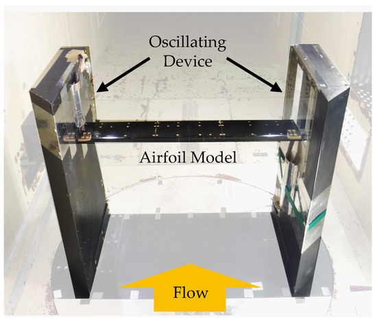
Figure 1.
Oscillating device and airfoil model installed in the test section.
The flow velocity in the test section was accelerated by the blockage effect. We confirmed that little disturbance exists around the airfoil model in the center of the test section by conducting the wind tunnel experiments without the airfoil model. A two-dimensional airfoil with a 12% airfoil thickness ratio, a 200-mm chord, and a 1000-mm span was used as a test model. The airfoil is designed for use as a helicopter blade. There were four kinds of pressure sensors (Kulite Semiconductor Products, Inc., XCQ-080-0.35BARG and XCQ-0935D; All Sensors Corp., 60INCH-D1-P4V-MINI and 60INCH-D2-P4V-MINI) inside the model. Figure 2 shows the shape of the airfoil model and the position of the sensors inside it.
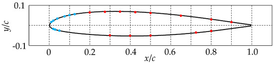
Figure 2.
Shape of the airfoil model and position of the sensors, where x and y are the parallel and normal components of the coordinates of the sensor position, respectively, and c is the chord length. Red and blue dots are available and unavailable sensors when the nanosecond-pulse-driven dielectric barrier discharge plasma actuator (ns-DBDPA) is installed, respectively.
The ns-DBDPA covered the sensors installed on the leading edge, and therefore, these sensors were unavailable when the ns-DBDPA was present. Because the airfoil model is made of synthetic wood, the model is insulated from the ns-DBDPA. Different discharge configurations of the ns-DBDPA were adopted. Figure 3a,b show electrode configurations of a double-discharge ns-DBDPA and a single-discharge ns-DBDPA, respectively.
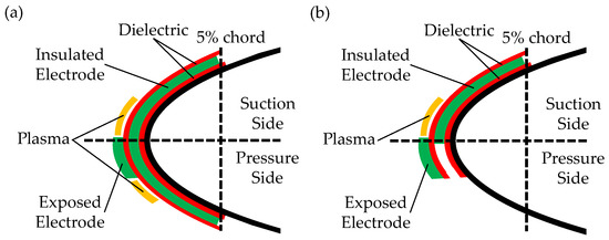
Figure 3.
Electrode configurations of (a) double-discharge ns-DBDPA and (a) single-discharge ns-DBDPA.
The ns-DBDPA is composed of a copper tape 0.055 mm thick (Lifework Concierge, LCA123), a copper tape 0.08 mm thick (Teraoka Seisakusho, 8323), and a polyimide film 0.07 mm thick (Teraoka Seisakusho, 650S #50), which correspond to an exposed electrode, an insulated electrode, and a dielectric, respectively. Plasma is generated by applying nanosecond voltage pulses to the exposed electrode and the insulated electrode sandwiched between the dielectric. Therefore, the discharge of the generated plasma can be controlled by changing the configuration. The double-discharge ns-DBDPA generates plasma on both the suction and pressure sides, and the single-discharge ns-DBDPA generates plasma on the suction side only. The best control effect is known to be obtained by generating plasma upstream of the separation point [11]. In dynamic stall flow, the separation point is known to change as the angle of attack changes. Therefore, in the double-discharge ns-DBDPA, the plasma was generated at 0% of the chord length on the pressure side. In the single-discharge ns-DBDPA, the position of the ns-DBDPA was moved downstream to investigate the best point for installation of the ns-DBDPA. We used a custom-designed pulse power source [26] to apply the voltage. Figure 4a,b show the voltage and current waveform of the nanosecond voltage pulse, respectively.
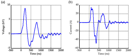
Figure 4.
(a) Voltage and (b) current waveforms of the nanosecond voltage pulse.
2.2. Experimental Conditions
Parameters were classified into oscillation and control parameters. The freestream velocity (m/s), the mean of the angle of attack (deg), and the reduced frequency k were chosen as the oscillation parameters. The ranges of these parameters were set to be similar to those in a helicopter flight environment, and the conditions under which a flow control effect was expected to appear were investigated. In these tests, was not realized correctly at the model position because of the blockage effect of the oscillating device. The actual velocity was obtained by particle image velocimetry data, and it was found to be from 44 m/s to 61 m/s, corresponding to Reynolds numbers, based on the chord length, from 6.0 × 10 to 8.3 × 10. The angle of attack (deg) at a certain time t (s) is calculated with the oscillation frequency f (Hz), (deg), and the oscillation amplitude (deg) as follows:
and k is calculated with the chord length c (m), (m/s) and f (Hz) as follows:
The nondimensional frequency of the pulse voltage , the peak pulse voltage , and the type and position of the ns-DBDPA were chosen as the control parameters. These parameters were varied over a wide range, and the conditions that maximize the flow control effect were investigated. Here, is calculated with the frequency of the pulse voltage (Hz), c (m), and (m/s) as follows:
The experimental conditions of the wind tunnel tests are shown in Table 1.

Table 1.
Parameter changes for each experimental condition.
Here, the experimental conditions of the wind tunnel test applied to investigate the reliability of the aerodynamic coefficients and the flow control effect are represented by Cases 1 and 2, respectively. The experimental conditions applied to investigate the flow control effect sensitivity are represented by Cases 3 to 11. In Case 5, the frequency of the pulse voltage during a single oscillation is kept constant, and therefore, increases as k increases. In these tests, was set 10 deg and the reason is shown in Appendix A.
2.3. Data Processing Method
Unsteady pressure was measured using 23 pressure sensors, as shown in Figure 2. The ns-DBDPA covered the sensors installed on the leading edge, and therefore, aerodynamic coefficients were calculated without the unavailable sensors when the ns-DBDPA was installed. Four kinds of pressure sensors were installed inside the model. High-frequency-response sensors (Kulite Semiconductor Products, Inc., XCQ-080-0.35BARG and XCQ-0935D) and low-frequency-response sensors (All Sensors Corp., 60INCH-D1-P4V-MINI and 60INCH-D2-P4V-MINI) were connected to low-pass filters with steepness values of 135 dB/oct (NF Corp., P-86) and 48 dB/oct (NF Corp., P-85 and 7295), respectively. The cutoff frequency of the low-pass filters is 1000 Hz. The low-pass filters were connected to two kinds of data loggers (Keyence Corp., NR600; National Instruments, cDAQ-9188). The sampling rate and the measurement time were 2000 Hz and 11 s, respectively. The timing of pulses driving the ns-DBDPA was adjusted to the same angle of attack in each oscillation cycle and the data were phase-averaged. Figure 5 shows the timing of pulses driving the ns-DBDPA.
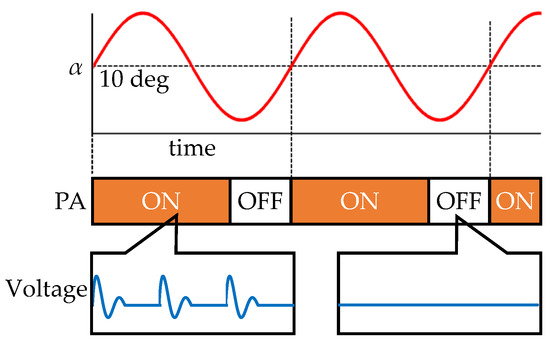
Figure 5.
Timing of pulses driving the ns-DBDPA.
The pulses driving the ns-DBDPA were initiated at 10 deg in the pitching-up phase of all cycles. The model was oscillated with f from 1.1 to 8 Hz, and therefore, at least 11 cycles were phase-averaged. The phase-averaged pressure data were used to calculate the pressure coefficient as follows:
where , , and p are the air density, the wind tunnel static pressure, and the phase-averaged pressure, respectively. The aerodynamic coefficients for lift , pressure drag , and pitching moment are calculated by integrating the distribution on the airfoil as follows:
where and are the horizontal and vertical distances between the neighboring sensors, respectively, and is the number of sensors.
3. Results and Discussion
3.1. Reliability of Aerodynamic Coefficients
Some pressure sensors were unavailable when the ns-DBDPA was installed on the airfoil’s leading edge. Therefore, aerodynamic coefficients calculated with and without the leading-edge sensors were compared and the reliability of the aerodynamic coefficients was evaluated. Figure 6 shows the distribution of the suction side with and without the leading-edge sensors. The distribution was obtained by linearly interpolating of the neighboring sensors. Figure 7 shows and with and without the leading-edge sensors. The movement of the model is divided into the pitching-up and pitching-down phases. In the pitching-up phase, gradually decreases and linearly increases beyond the static stall angle. Therefore, the flow separation seems to be delayed. At the moment when the model changes from the pitching-up to pitching-down phase, the location where decreases moves from the leading edge to the trailing edge and clearly changes. Therefore, the vortex seems to be generated on the leading edge and convected downstream. In the pitching-down phase until approximately 11 deg, gradually increases and decreases. Therefore, the flow seems to be separated. Suddenly, on the leading edge decreases and increases. Therefore, the flow seems to be attached. Dynamic stall flow is known to cause delayed flow separation beyond the static stall angle, the generation of the dynamic stall vortices, and delayed flow attachment below the static stall angle [4]; therefore, dynamic stall flow was observed in these experiments. Here, the distribution is similar to that in previous experiments [27] conducted with a Reynolds number, based on a chord length of 3.0 × 10 and k of 0.050.
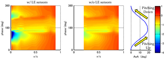
Figure 6.
Pressure coefficient distribution of the suction side, which is calculated with and without leading-edge (LE) sensors when the ns-DBDPA is not installed. The experimental conditions are shown in Case 1 in Table 1.
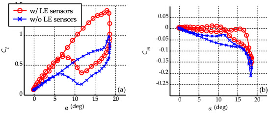
Figure 7.
(a) Lift coefficient and (b) pitching moment coefficient calculated with and without leading-edge (LE) sensors when the ns-DBDPA is not installed.
When the leading-edge sensors are blocked, the peak is not observed. However, a decrease in on the suction side at the moment when the model changes from pitching up to pitching down is observed. Therefore, the dynamic stall vortex was resolved. and in both cases are different, and therefore, it is difficult to evaluate the aerodynamic coefficients quantitatively when the suction peak is not resolved. The predominant differences in both cases are the slope of in the pitching-up phase and the peak of at the moment when the model changes from pitching up to pitching down. In the pitching-down phase, the peak is not observed, and therefore, the influence of the lack of the pressure sensors on the leading edge to qualitative evaluations of and are considered to be small. The trends of in both cases are qualitatively similar, though it should be noted that is underestimated overall and the effect of the vortex is overestimated when the suction peak is not resolved. Similarly, in both cases is qualitatively different compared with . This might be because is more sensitive to the suction peak of the pressure. The evaluation of the value of is difficult because of lack of pressure sensors on the leading edge, and it is just shown as reference data [24]. Therefore, we evaluated the control effect qualitatively using rather than . It is difficult to evaluate the error of and in the present study, and therefore, the flow control effect is evaluated qualitatively. A more quantitative discussion is left for a future study.
3.2. Flow Control Effect
The aerodynamic coefficients with and without driving the ns-DBDPA are compared, and the flow control effect was investigated. Figure 8 shows the distribution on the suction side in the cases with and without driving the ns-DBDPA. Figure 9a–c show , , and , respectively, in the cases with and without driving the ns-DBDPA. and are defined as the lift coefficients in the pitching-up and pitching-down phases, respectively. The distribution in the pitching-up phase and that in the pitching-down phase are different. The difference results in hysteresis of the aerodynamic coefficients. A comparison of the two conditions shows that there is little difference in the distribution except during the pitching-down phase. In the pitching-down phase, when the ns-DBDPA is driven, locations where decreases appear repeatedly. Therefore, when the ns-DBDPA is driven is clearly larger than that when the ns-DBDPA is not driven. As a result, the ns-DBDPA can reduce the hysteresis of . Not only the hysteresis of but also the hystereses of and are reduced by driving the ns-DBDPA. The flow control effect is evaluated using the efficiency of the lift enhancement [15] as follows:
where w/ PA and w/o PA are the cases with and without driving the ns-DBDPA, respectively. increases as the hysteresis decreases when the ns-DBDPA is driven. The lift enhancement effect, which is produced when driving the ns-DBDPA, is accompanied by the fluctuation of these coefficients. The frequency of the fluctuation corresponds to . This result indicates that the fluctuation is caused by the vortices generated when the ns-DBDPA is driven. Here, vortices are considered to be generated by driving the ns-DBDPA installed on the leading edge of the NACA0015 airfoil model; therefore, a similar phenomenon to that in the previous study [27] seems to be observed in the flow fields around the oscillating airfoil in the present study. In a previous study, Post et al. also reported that the flow separation control is effective in the pitching-down phase because the disturbance at the leading edge brings high momentum flow near the surface [13]. Moreover, the leading-edge vortex is formed and induces the lift. It should be noted that the flow control effect is observed in the pitching-down phase and the influence of the leading-edge sensors to the qualitative evaluation of is small. Therefore, it is possible to discuss the qualitative effect of the control without the leading-edge sensors.
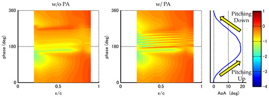
Figure 8.
Pressure coefficient distribution of the suction side in the cases with and without driving the ns-DBDPA. The experimental conditions are shown in Case 2 in Table 1.
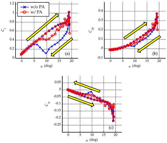
Figure 9.
(a) Lift coefficient, (b) pressure drag coefficient, and (c) pitching moment coefficient in the cases with and without driving the ns-DBDPA.
3.3. Flow Control Effect Sensitivity of Parameters
The different values of aerodynamic coefficients that change the oscillation and control parameters are compared, and the sensitivity of the flow control effect to these parameters is investigated.
3.3.1. Freestream Velocity
Figure 10a,b show under different conditions in the cases without and with driving the ns-DBDPA, respectively. When the ns-DBDPA is not driven, does not change as increases. However, with m/s is the smallest of the three cases. The flow control effect appears in all the cases. However, the phase of the fluctuation of differs. increases as increases while keeping constant, and therefore, the phase difference is caused by the difference in . Figure 11 shows the effect of on . There is little difference between with m/s and m/s, so the sensitivity of to is low. The flow control effect of the ns-DBDPA is expected to appear at higher freestream velocities.

Figure 10.
Lift coefficients under different freestream velocity conditions. Here, (a,b) correspond to without and with driving the ns-DBDPA, respectively. The experimental conditions are shown in Case 3 in Table 1.
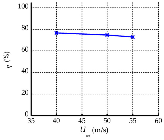
Figure 11.
Effect of the freestream velocity on the efficiency of the lift enhancement.
3.3.2. Mean of the Angle of Attack
Figure 12a,b show under different conditions in the cases without and with driving the ns-DBDPA, respectively. When the ns-DBDPA is not driven, with deg is smaller than that with deg, and therefore, the hysteresis is exacerbated as increases. When the ns-DBDPA is driven, the hysteresis is also exacerbated as increases. In both cases with deg, fluctuations in are observed. This result indicates that the peaks are caused by the dynamic stall vortices. clearly increases when the ns-DBDPA is driven, while does not change. This result indicates that the ns-DBDPA has little effect on the dynamic stall vortex. Figure 13 shows the effect of on , which decreases as increases.
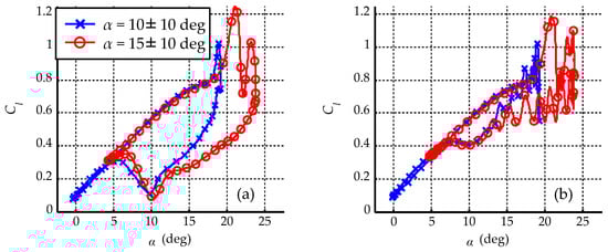
Figure 12.
Lift coefficients under different means of the angle of attack. Here, (a,b) correspond to without and with driving the ns-DBDPA, respectively. The experimental conditions are shown in Case 4 in Table 1.
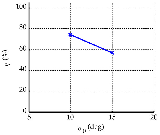
Figure 13.
Effect of the mean of the angle of attack on the efficiency of the lift enhancement.
3.3.3. Reduced Frequency
Figure 14a,b show under different k conditions in the cases without and with driving the ns-DBDPA, respectively. When the ns-DBDPA is not driven, the hysteresis is exacerbated as k increases. When the flow around the airfoil is attached, changes linearly. Therefore, the range of at which the flow is attached decreases as k increases. with k = 0.004 does not increase linearly because the flow is separated. The flow control effect appears in all the cases. Especially, at k = 0.004 dramatically increases when the ns-DBDPA is driven. Figure 15 shows the effect of k on . The flow control effect appears in all the cases, but decreases as k increases. at k = 0.004 exceeds 100% because the hysteresis of becomes larger with driving the ns-DBDPA than that without driving ns-DBDPA.
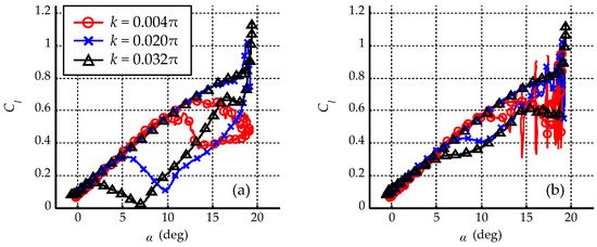
Figure 14.
Lift coefficients under different reduced frequency conditions. Here, (a,b) correspond to without and with driving the ns-DBDPA, respectively. The experimental conditions are shown in Case 5 in Table 1.
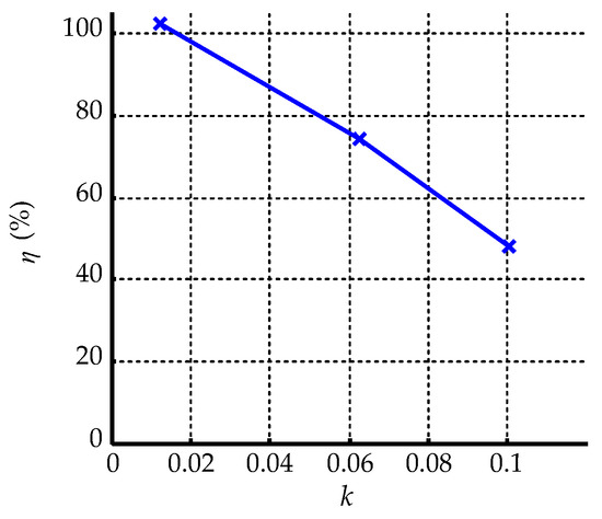
Figure 15.
Effect of the reduced frequency on the efficiency of the lift enhancement.
3.3.4. Nondimensional Frequency of Pulse Voltage
Figure 16a,b show under different conditions when k is 0.020 and 0.032, respectively. Figure 17 shows the effect of on , which increases as decreases. Thus, a lower is effective for flow control in the range investigated. However, the flow control effect is estimated to decrease as further decreases when is less than 0.5 because the vortices that affects the lift enhancement mechanism does not seem to be formed on the airfoil. Although additional tests over a wider frequency range are required for the investigation of the optimal , the best flow control effect is obtained with an of 0.5 in the range we investigated. In both cases, clearly increases when the ns-DBDPA is driven. Moreover, the amplitude of the fluctuation decreases and the frequency of the fluctuation increases as increases. This result indicates that is influenced by the vortices generated by the ns-DBDPA. A trade-off relationship exists between and the amplitude of the fluctuation. Similar phenomena were observed in the dynamic stall flow around the NACA0012 airfoil, and Singhal et al. reported that the fluctuation was observed at low numbers [27].
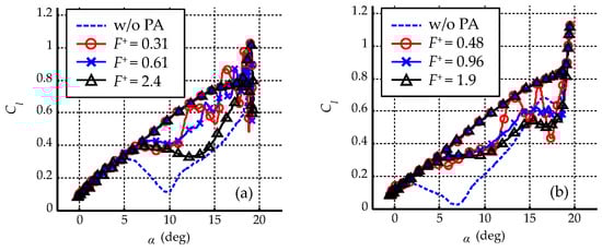
Figure 16.
Lift coefficients with different nondimensional frequency of pulse-voltage conditions when the reduced frequency is (a) 0.020 and (b) 0.032. The experimental conditions are shown in Cases 6 and 7 in Table 1.
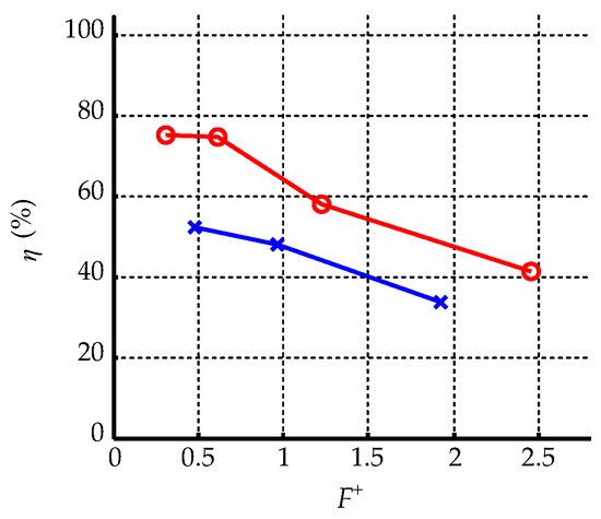
Figure 17.
Effect of the nondimensional frequency of the pulse voltage on the efficiency of the lift enhancement.
3.3.5. Peak Pulse Voltage
Figure 18 shows under different conditions. with = 2 kV is smaller than with = 3 kV. Figure 19 shows the effect of on . does not change as changes when is larger than 2 kV. When a higher is applied, more heat is produced by the generation of plasma. This result indicates that the flow control effect does not change very much, provided that a sufficient amount of heat is input and vortices are generated. A of 3 kV is efficient, considering the flow control effect and the power consumption.
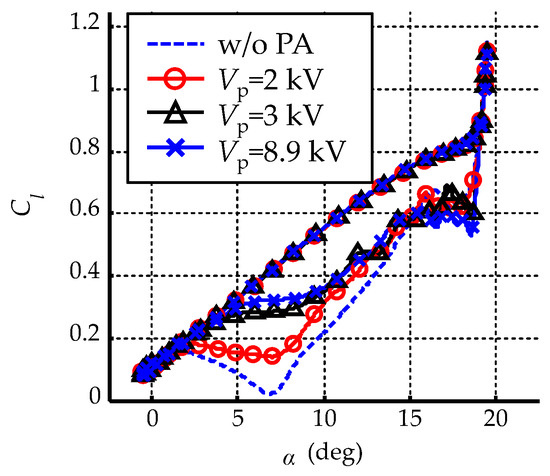
Figure 18.
Lift coefficients under different peak pulse-voltage conditions. The experimental conditions are shown in Case 8 in Table 1.
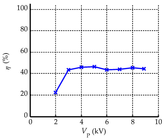
Figure 19.
Effect of the peak pulse voltage on the efficiency of the lift enhancement.
3.3.6. Type of ns-DBDPA
Figure 20a,b show with different types of ns-DBDPA when is 0.48 and 0.96, respectively. When the ns-DBDPA is not driven, does not differ between the ns-DBDPA types, but in the single-discharge ns-DBDPA is larger than in the double-discharge ns-DBDPA. The shape of the leading edge differs between the two types, as shown in Figure 3, and therefore, the shape influences the separated flow at a high angle of attack. Similarly, in the single-discharge ns-DBDPA is also larger than that in the double-discharge ns-DBDPA when the ns-DBDPA is driven. Therefore, the single-discharge ns-DBDPA shows a higher flow control effect regardless of whether the ns-DBDPA is driven. The ns-DBDPA also acts as a passive flow control device under these conditions. Figure 21 shows the effect of the ns-DBDPA types on . in the single-discharge ns-DBDPA is larger than that in the double-discharge ns-DBDPA. In summary, a high flow control effect is obtained in the single-discharge ns-DBDPA, and this is caused by not only the difference in the disturbance added by the ns-DBDPA but also the different shapes of the ns-DBDPA types.
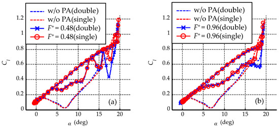
Figure 20.
Lift coefficients with different types of ns-DBDPA when the nondimensional frequency of the pulse voltage is (a) 0.48 and (b) 0.96. The experimental conditions are shown in Cases 9 and 10 in Table 1.
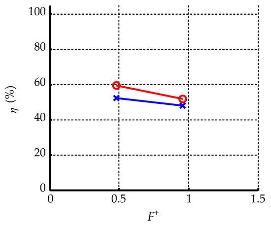
Figure 21.
Effect of the ns-DBDPA type on the efficiency of the lift enhancement.
3.3.7. Position of ns-DBDPA
Figure 22a,b show under different conditions in the cases without and with driving the ns-DBDPA, respectively. and the peak of at the moment when the model changes from pitching up to pitching down changes as changes when the ns-DBDPA is not driven. The shape of the leading edge changes as changes, and therefore, the shape difference influences the separated flow and the dynamic stall vortex. The result also shows that the ns-DBDPA also acts as a passive flow control device. When the ns-DBDPA is driven, changes as changes. The flow control effect is also sensitive to the shape of the leading edge. Figure 23 shows the effect of on . When is 0%, is the highest among the three cases; therefore, an of 0% seems to be the most effective.
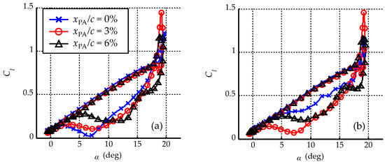
Figure 22.
Lift coefficient under different ns-DBDPA positions. Here, (a,b) correspond to without and with driving the ns-DBDPA, respectively. The experimental conditions are shown in Case 11 in Table 1.
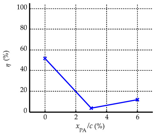
Figure 23.
Effect of the position of the ns-DBDPA on the efficiency of the lift enhancement.
4. Conclusions
In the present study, unsteady pressure was measured in a wind tunnel using the ns-DBDPA as a flow control device. The flow control effect and its sensitivity to the pitching oscillation and ns-DBDPA control parameters were investigated. The freestream velocity, the mean of the angle of attack, and the reduced frequency were employed as the oscillation parameters. Moreover, the nondimensional frequency of the pulse voltage, the peak pulse voltage, and the type and position of the ns-DBDPA were adopted as the control parameters. The ns-DBDPA was installed on the leading edge of an airfoil model that was in the form of a helicopter blade. The model was oscillated periodically around 25% of the chord length. Aerodynamic coefficients were calculated by integrating the pressure distribution that was measured by pressure sensors inside the model. The aerodynamic coefficients are discussed qualitatively because the suction peak was not resolved. Overall, the lift coefficient was underestimated and the effect of the vortex was overestimated.
The results related to the flow control effect are summarized below:
- The lift coefficient increases by driving the ns-DBDPA when the model is pitching down;
- The aerodynamic coefficients corresponding to the frequency of the pulse voltage fluctuate when the ns-DBDPA is applied.
The effects of the model oscillation parameters on the flow control effect are summarized below:
- The flow control effect appears under all conditions in which the freestream velocity, the angle of attack, and the reduced frequency were set to be from 40 m/s to 55 m/s, from 10 ± 10 deg to 15 ± 10 deg, and from 0.004 to 0.032, respectively;
- Changes in the freestream velocity have little effect on the flow control effect in the range we investigated;
- The flow control effect increases as the mean of the angle of attack and the reduced frequency decrease.
The effects of the ns-DBDPA control parameters on the flow control effect are summarized below:
- The flow control effect increases as the nondimensional frequency of the pulse voltage decreases in the range we investigated, but the amplitude of the lift coefficient fluctuation increases;
- A sufficient flow control effect is obtained when the peak pulse voltage is greater than or equal to 3 kV;
- The flow control effect is sensitive to the shape of the leading edge. The best flow control effect is obtained when the position of the ns-DBDPA is 0% in the single-discharge type in the range we investigated.
Author Contributions
Conceptualization, T.N. (Taku Nonomura), K.A., A.K., A.A., K.T., T.K., K.H. and K.N. (Kazuyuki Nakakita); data curation, Y.I. and T.N. (Taku Nonomura); formal analysis, Y.I. and T.N. (Taku Nonomura); funding acquisition, H.Y., K.H. and T.T.; investigation, Y.I., T.N. (Taku Nonomura), K.N. (Koki Nankai), S.K., K.S., A.K., H.Y., K.H., T.N. (Tsutomu Nakajima) and K.N. (Kazuyuki Nakakita); project administration, H.Y., K.H. and T.T.; resources, S.K., K.S., A.K., A.A., K.T., T.K., H.Y., K.H., T.T., T.N. (Tsutomu Nakajima) and K.N. (Kazuyuki Nakakita); software, Y.I., T.N. (Taku Nonomura) and K.N. (Koki Nankai); supervision, T.N. (Taku Nonomura) and K.A.; visualization, Y.I. and T.N. (Taku Nonomura); writing–original draft preparation, Y.I.; writing–review and editing, Y.I. and T.N. (Taku Nonomura). All authors have read and agreed to the published version of the manuscript.
Funding
This research received no external funding.
Acknowledgments
The authors would like to express their gratitude to K. Mitsuo who generously permitted us to use an oscillating machine that he made.
Conflicts of Interest
The authors declare no conflict of interest.
Appendix A. Selection of Oscillating Amplitude
We conducted the experiment to select the oscillating amplitude where the dynamic stall appears. The experimental conditions of the wind tunnel tests are shown in Table A1.
Table A1.
The experimental conditions changing the oscillating amplitude.
Table A1.
The experimental conditions changing the oscillating amplitude.
| (m/s) | (deg) | (deg) | k |
|---|---|---|---|
| 50 | 8–10 | 8–10 | 0.032 |
Figure A1 shows under different conditions when the ns-DBDPA is not driven. The peak of decreases as the maximum angle of attack decreases. Therefore, the influence of the dynamic stall vortex decreases as the maximum angle of attack decreases. In the experiments, the oscillation amplitude was set 10 deg.

Figure A1.
Lift coefficients under different oscillation amplitude conditions when the ns-DBDPA is not driven. The experimental conditions are shown in Table A1.
Figure A1.
Lift coefficients under different oscillation amplitude conditions when the ns-DBDPA is not driven. The experimental conditions are shown in Table A1.

References
- McCroskey, W.J. The Phenomenon of Dynamic Stall; Technical Report; National Aeronuatics and Space Administration Moffett Field Ca Ames Research Center: Washington, DC, USA, 1981. [Google Scholar]
- Carr, L.W. Progress in analysis and prediction of dynamic stall. J. Airc. 1988, 25, 6–17. [Google Scholar] [CrossRef]
- Wang, S.; Ingham, D.B.; Ma, L.; Pourkashanian, M.; Tao, Z. Numerical investigations on dynamic stall of low Reynolds number flow around oscillating airfoils. Comput. Fluids 2010, 39, 1529–1541. [Google Scholar] [CrossRef]
- Corke, T.C.; Thomas, F.O. Dynamic stall in pitching airfoils: Aerodynamic damping and compressibility effects. Annu. Rev. Fluid Mech. 2015, 47, 479–505. [Google Scholar] [CrossRef]
- Nankai, K.; Ozawa, Y.; Nonomura, T.; Asai, K. Linear Reduced-order Model Based on PIV Data of Flow Field around Airfoil. Trans. Jpn. Soc. Aeronaut. Space Sci. 2019, 62, 227–235. [Google Scholar] [CrossRef]
- Zong, H.; Chiatto, M.; Kotsonis, M.; de Luca, L. Plasma synthetic jet actuators for active flow control. Actuators 2018, 7, 77. [Google Scholar] [CrossRef]
- Zong, H.; Kotsonis, M. Formation, evolution and scaling of plasma synthetic jets. J. Fluid Mech. 2018, 837, 147–181. [Google Scholar] [CrossRef]
- Roth, J.R. Aerodynamic flow acceleration using paraelectric and peristaltic electrohydrodynamic effects of a one atmosphere uniform glow discharge plasma. Phys. Plasmas 2003, 10, 2117–2126. [Google Scholar] [CrossRef]
- Post, M.L.; Corke, T.C. Separation control on high angle of attack airfoil using plasma actuators. AIAA J. 2004, 42, 2177–2184. [Google Scholar] [CrossRef]
- Forte, M.; Leger, L.; Pons, J.; Moreau, E.; Touchard, G. Plasma actuators for airflow control: Measurement of the non-stationary induced flow velocity. J. Electrostat. 2005, 63, 929–936. [Google Scholar] [CrossRef]
- Sato, M.; Aono, H.; Yakeno, A.; Nonomura, T.; Fujii, K.; Okada, K.; Asada, K. Multifactorial effects of operating conditions of dielectric-barrier-discharge plasma actuator on laminar-separated-flow control. AIAA J. 2015, 53, 2544–2559. [Google Scholar] [CrossRef]
- Sekimoto, S.; Nonomura, T.; Fujii, K. Burst-mode frequency effects of dielectric barrier discharge plasma actuator for separation control. AIAA J. 2017, 1385–1392. [Google Scholar] [CrossRef]
- Post, M.L.; Corke, T.C. Separation control using plasma actuators: Dynamic stall vortex control on oscillating airfoil. AIAA J. 2006, 44, 3125–3135. [Google Scholar] [CrossRef]
- Greenblatt, D.; Ben-Harav, A.; Mueller-Vahl, H. Dynamic stall control on a vertical-axis wind turbine using plasma actuators. AIAA J. 2014, 52, 456–462. [Google Scholar] [CrossRef]
- Mitsuo, K.; Watanabe, S.; Atobe, T.; Kato, H.; Tanaka, M.; Uchida, T. Lift Enhancement of a Pitching Airfoil in Dynamic Stall by DBD Plasma Actuators. In Proceedings of the 51st AIAA Aerospace Sciences Meeting Including the New Horizons Forum and Aerospace Exposition, Grapevine, TX, USA, 7–10 January 2013; p. 1119. [Google Scholar]
- Guoqiang, L.; Weiguo, Z.; Yubiao, J.; Pengyu, Y. Experimental investigation of dynamic stall flow control for wind turbine airfoils using a plasma actuator. Energy 2019, 185, 90–101. [Google Scholar] [CrossRef]
- Roupassov, D.; Nikipelov, A.; Nudnova, M.; Starikovskii, A.Y. Flow separation control by plasma actuator with nanosecond pulsed-periodic discharge. AIAA J. 2009, 47, 168–185. [Google Scholar] [CrossRef]
- Little, J.; Takashima, K.; Nishihara, M.; Adamovich, I.; Samimy, M. Separation control with nanosecond-pulse-driven dielectric barrier discharge plasma actuators. AIAA J. 2012, 50, 350–365. [Google Scholar] [CrossRef]
- Kelley, C.L.; Bowles, P.O.; Cooney, J.; He, C.; Corke, T.C.; Osborne, B.A.; Silkey, J.S.; Zehnle, J. Leading-edge separation control using alternating-current and nanosecond-pulse plasma actuators. AIAA J. 2014, 52, 1871–1884. [Google Scholar] [CrossRef]
- Little, J.; Singh, A.; Ashcraft, T.; Durasiewicz, C. Post-stall flow control using nanosecond pulse driven dielectric barrier discharge plasma actuators. Plasma Sources Sci. Technol. 2018, 28, 014002. [Google Scholar] [CrossRef]
- Zhang, C.; Huang, B.; Luo, Z.; Che, X.; Yan, P.; Shao, T. Atmospheric-pressure pulsed plasma actuators for flow control: Shock wave and vortex characteristics. Plasma Sources Sci. Technol. 2019, 28, 064001. [Google Scholar] [CrossRef]
- Starikovskiy, A.; Meehan, K.; Persikov, N.; Miles, R. Static and dynamic stall control by NS SDBD actuators. Plasma Sources Sci. Technol. 2019, 28, 054001. [Google Scholar] [CrossRef]
- Komuro, A.; Takashima, K.; Konno, K.; Tanaka, N.; Nonomura, T.; Kaneko, T.; Ando, A.; Asai, K. Schlieren visualization of flow-field modification over an airfoil by near-surface gas-density perturbations generated by a nanosecond-pulse-driven plasma actuator. J. Phys. D Appl. Phys. 2017, 50, 215202. [Google Scholar] [CrossRef]
- Frankhouser, M.W.; Gregory, J.W. Nanosecond Dielectric Barrier Discharge Plasma Actuator Flow Control of Compressible Dynamic Stall. In Proceedings of the 46th AIAA Plasmadynamics and Lasers Conference, Dallas, TX, USA, 22–26 June 2015; p. 2341. [Google Scholar]
- Fukumoto, H.; Aono, H.; Watanabe, T.; Tanaka, M.; Matsuda, H.; Osako, T.; Nonomura, T.; Oyama, A.; Fujii, K. Control of dynamic flowfield around a pitching NACA633- 618 airfoil by a DBD plasma actuator. Int. J. Heat Fluid Flow 2016, 62, 10–23. [Google Scholar] [CrossRef]
- Komuro, A.; Takashima, K.; Suzuki, K.; Kanno, S.; Nonomura, T.; Kaneko, T.; Ando, A.; Asai, K. Influence of discharge energy on the lift and drag forces induced by a nanosecond-pulse-driven plasma actuator. Plasma Sources Sci. Technol. 2019, 28, 065006. [Google Scholar] [CrossRef]
- Singhal, A.; Castañeda, D.; Webb, N.; Samimy, M. Control of dynamic stall over a NACA 0015 airfoil using plasma actuators. AIAA J. 2017, 78–89. [Google Scholar] [CrossRef]


© 2020 by the authors. Licensee MDPI, Basel, Switzerland. This article is an open access article distributed under the terms and conditions of the Creative Commons Attribution (CC BY) license (http://creativecommons.org/licenses/by/4.0/).