Article

Heavy Oil Laminar Flow in Corrugated Ducts: A Numerical Study Using the Galerkin-Based Integral Method

by
Valdecir Alves dos Santos Júnior
1,*,
Severino Rodrigues de Farias Neto
2,
Antonio Gilson Barbosa de Lima
3,
Igor Fernandes Gomes
4,
Israel Buriti Galvão
5,
Célia Maria Rufino Franco
6 and
João Evangelista Franco do Carmo
7
1
Department of Physics and Civil Engineering, Center of Science, Technology and Health, State University of Paraíba, Cel. Pedro Targino Ave, 58233-000 Araruna-PB, Brazil
2
Department of Chemical Engineering, Center of Science and Technology, Federal University of Campina Grande, 882 Aprígio Veloso St, 58428-830 Campina Grande-PB, Brazil
3
Department of Mechanical Engineering, Center of Science and Technology, Federal University of Campina Grande, 882 Aprígio Veloso St, 58428-830 Campina Grande-PB, Brazil
4
Department of Civil Engineering, Technology Center, Federal University of Pernambuco, Acadêmico Hélio Ramos St, 50670-420 Recife-PE, Brazil
5
Department of Mathematics, Center of Science and Technology, State University of Paraíba, 351 Baraúnas St, 58429-500 Campina Grande-PB, Brazil
6
Department of Physics and Mathematics, Federal University of Campina Grande, 58175-000 Cuité-PB, Brazil
7
Department of Mechanical Engineering, Federal University of Campina Grande, 58429-900 Campina Grande-PB, Brazil
*
Author to whom correspondence should be addressed.
Energies 2020, 13(6), 1363; https://doi.org/10.3390/en13061363
Submission received: 20 February 2020 / Revised: 6 March 2020 / Accepted: 10 March 2020 / Published: 15 March 2020

Abstract

:
Fluid flow in pipes plays an important role in different areas of academia and industry. Due to the importance of this kind of flow, several studies have involved circular cylindrical pipes. This paper aims to study fully developed internal laminar flow through a corrugated cylindrical duct, using the Galerkin-based integral method. As an application, we present a study using heavy oil with a relative density of 0.9648 (14.6 °API) and temperature-dependent viscosities ranging from 1715 to 13000 cP. Results for different fluid dynamics parameters, such as the Fanning friction factor, Reynolds number, shear stress, and pressure gradient, are presented and analyzed based on the corrugation number established for each section and aspect ratio of the pipe.

1. Introduction

The oil industry is a major player in the energy sector worldwide. The increased demand for light oil reserves in recent decades has led to their depletion. As a result, heavy oil is increasingly a topic of interest, receiving considerable attention regarding its efficient transportation. Although there is a large amount of productive crude oil reserves, heavy oil transportation is a complex and expensive task due to its high viscosity, which requires a large amount of energy to pump [1].
One of the major concerns in the production and transportation of heavy oil is related to load loss or pressure drops, which are associated with high flow costs. This occurs due to the fluid friction effect on the inner walls of the duct, making its transport difficult, and increasing the refining cost [2]. Currently, different methods are employed to transport heavy oil from the production field to refineries and markets. Although many other options are available, pipelines are the safest, most efficient, and financially viable means of transporting heavy oil [3].
For many years, analytical and numerical solutions applied to fluid flow inside ducts with arbitrary cross-sections have been studied. Aparecido and Cotta [4] applied generalized integral transform techniques to find solutions for forced laminar convection in rectangular ducts. The same authors, in 1991, presented a generalized integral transform technique for forced laminar convection solutions at the thermal entrance region of ducts with arbitrary cross-sections. Syrjala [5] performed a numerical study related to the laminar flow behavior of viscoelastic fluids in rectangular ducts using the finite element method. Aparecido and Lindquist [6] analytically studied a Newtonian fluid over laminar flow, developed hydrodynamically and thermally, by using generalized integral transformation techniques, with axial and uniform heat flow in straight rectangular ducts. Lee and Kuo [7] applied the Galerkin-based integral method to calculate the Nusselt number for laminar flow in elliptical ducts imposed on the constant duct wall temperature. Values for the coefficient of friction were also found for elliptical ducts with and without a central circular core.
How much to transport of heavy oils, several techniques are employed. These include heat addition, light oil dilution, emulsion formation, and lubrication of the pipe walls with a lower viscosity fluid, all with the aim to reduce the pressure drop along the duct. For transporting a 17.6 Pa·s viscosity oil with a density of 963 kg/m3 at room temperature using the core-flow technique, Prada and Bannwart [8] found a reduction in the total pressure gradient between 45 and 150 times, compared to that obtained when the oil seeped alone into the pipe. Bensakhria et al. [9] experimentally evaluated the transport of heavy oil with a viscosity of 4.74 Pa·s at a constant temperature of 19.7 °C. The authors observed a reduction in pressure, with a drop of over 90% compared to that obtained with the same oil flowing without parietal lubrication, i.e., without applying the core-flow technique. These authors also observed that the difference in density between water and oil plays an important role in the flow behavior.
Thus, both numerical and experimental simulations are increasingly used to investigate in detail the local dynamics of fluid flow in pipelines, and in particular the importance of transporting heavy oil in this type of modal.
Given the real importance of this problem, in this paper, we propose to carry out a study on the fully developed laminar flow of heavy oil in corrugated cross-section ducts, presenting results for fluid dynamic parameters such as the Poiseuille number, Fanning friction factor, velocity, pressure gradient, shear stress, and Reynolds number, from the solution of the dimensionless momentum equation given by the Galerkin-based integral method, and considering temperature-dependent viscosity. When considering corrugated geometry, there are few works found in the literature. Among these few works, we can cite Casarella et al. [10], Hu and Chang [11], Moharana and Khandekar [12], and Shah [13]. Unfortunately, no work is applied to the petroleum industry.
The motivation for this research is related to the scarcity of work considering this geometry. Among these few works, we have the work of Hu and Chang [11] as a starting point. This work analyzes the fully developed flow over corrugated sine ducts. These authors employed the conformal mapping method and Green’s functions to determine f R e and N u H 1 . Different from the work of Hu and Chang, where the perimeter is calculated numerically, our work finds the perimeter by the arc length function. This function gives us an exact numeric value of the perimeter. Hu and Chang [11] also applied a perturbation method, the Galerkin internal variational method, and an integral contour equation method to analyze the same problem for corrugated ducts. They found that the perturbation method produced good results for minor disturbances. When the disturbance was large, the results were useful only for qualitative trends. In our research, we use serial approximations of the parameterization of the curve that represents the cross-section of the pipe, because such approximation results in computational gains.
Further, the Galerkin-based integral method has been successfully applied in algorithms in the fields of differential equations [12,13,14], analysis [15], mechanics, thermodynamics and hydrodynamics [16,17,18,19], and also in other engineering fields [20,21]. Specifically, in the calculation of the temperature and/or velocity in ducts, we can cite works with circular, rectangular, isosceles triangular, right triangular, and annuli cross-sections [22,23,24].

2. Mathematical Formulation

In this work, we choose the cylindrical coordinate system ( r ,   θ ,   z ) for the mathematical formulation of the physical problem, and the following assumptions are considered:
(a)
The laminar flow is fully developed, isothermal, single-phase, and steady-state;
(b)
The cross-sectional area of the tube, along the z-axis, is constant;
(c)
The properties of the fluid, thermal and physical, are considered constant;
(d)
There is a condition of not-slipping on the duct wall.
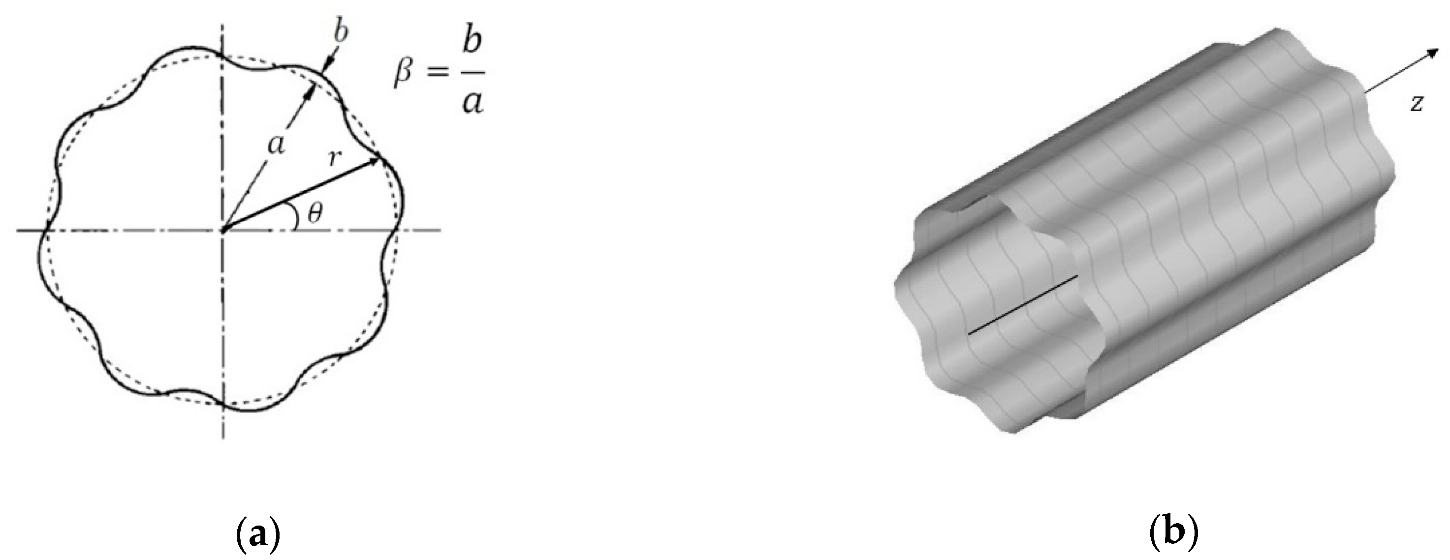
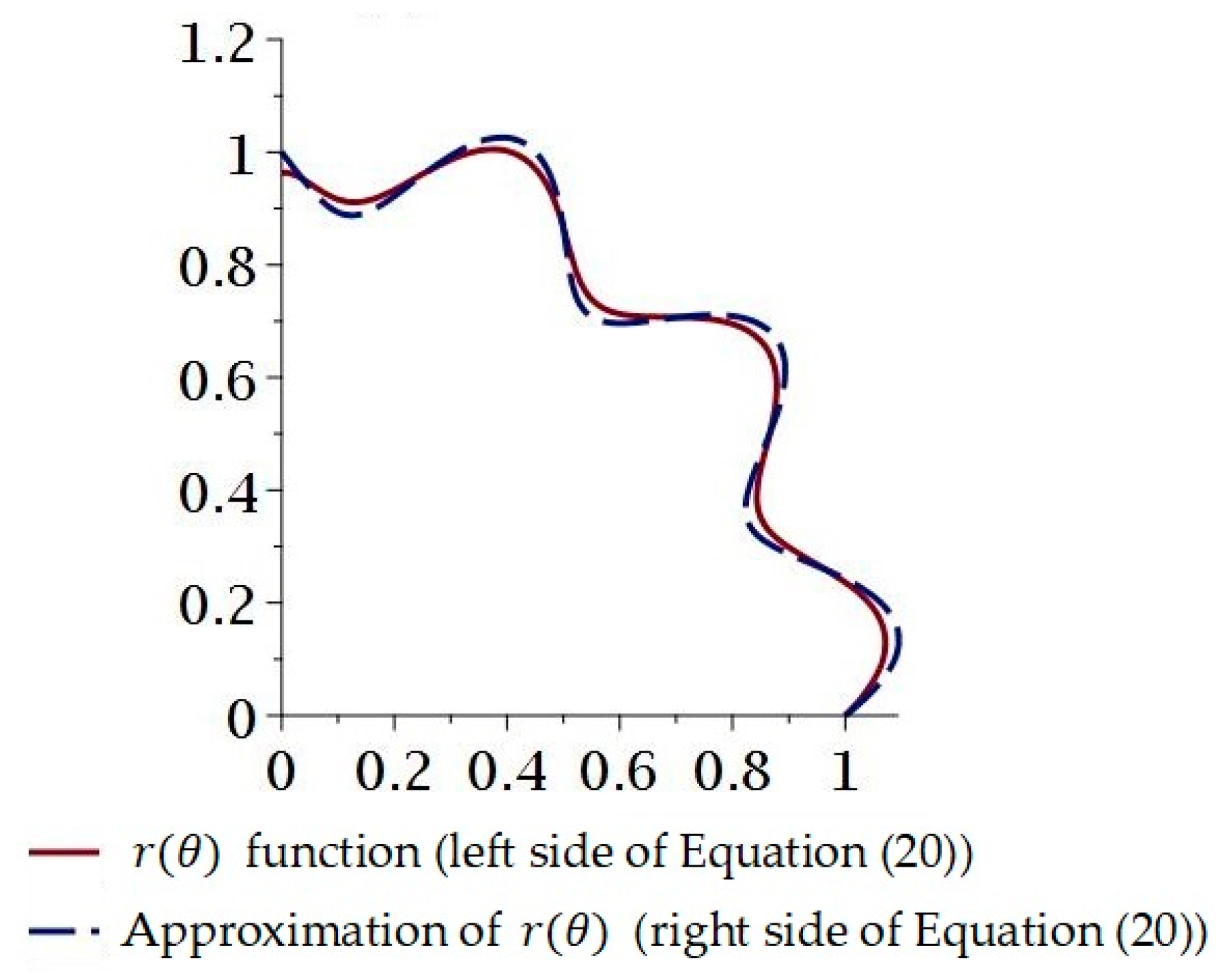
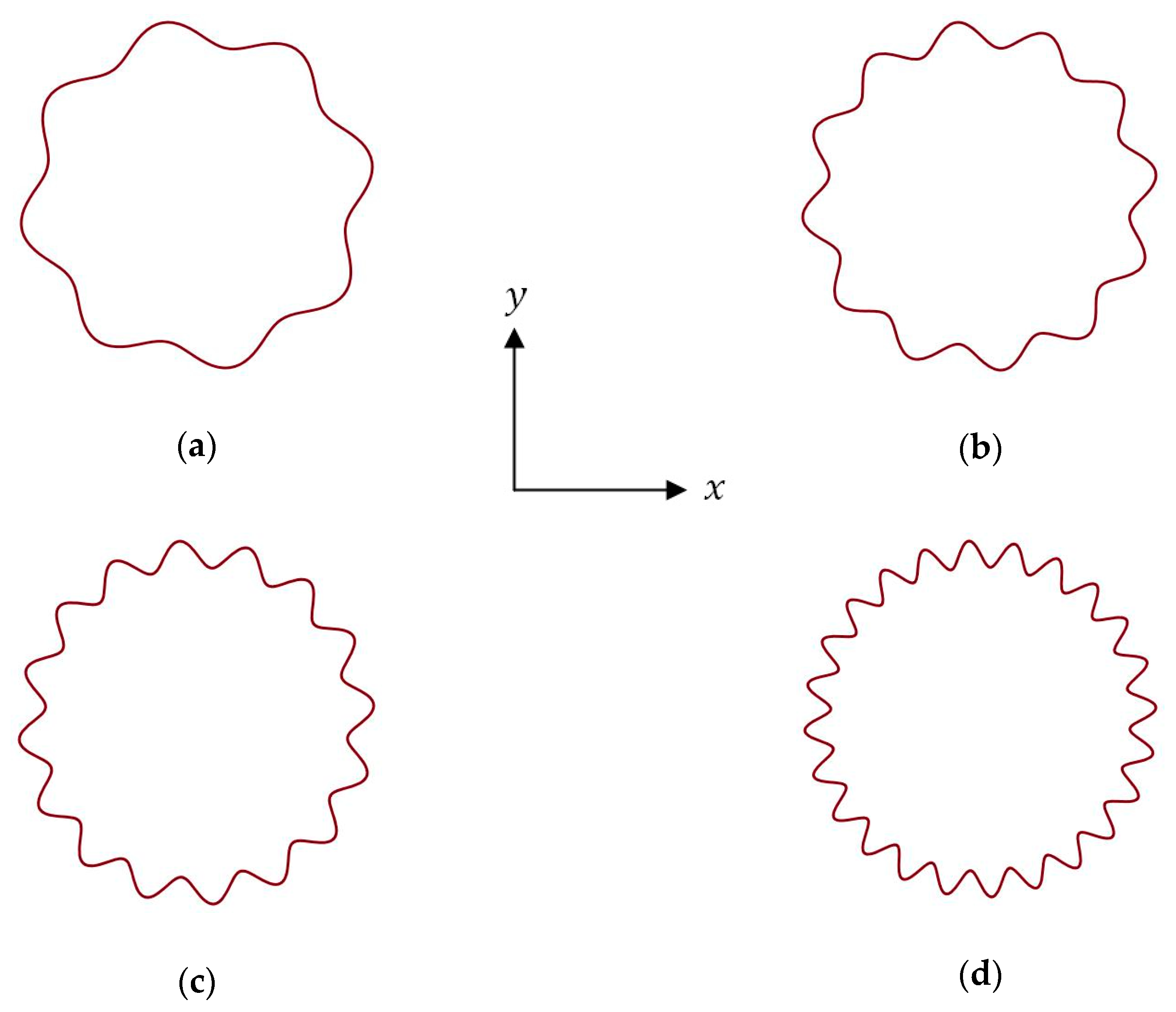
2.1. The Geometry

The geometry to be analyzed is a corrugated cylindrical duct. For a duct with corrugated geometry we consider, in polar coordinates, the parameterization of the cross-section, r ( θ ) = a + b   s i n ( N   θ ) , where a and b are shown in Figure 1 and N is the number of corrugations, sine-type. The relationship a b is the so-called aspect ratio,
Thus, considering the cross-section of the duct with the parameterization as reported before, the cross-sectional area of the duct is given as follows:
A c = 1 2 0 2 π [ a + b   sin ( N θ ) ] d θ ,
For the perimeter of the cross-section of the duct, we use the definition of arc length as follows:
P = 0 2 π [ a + b s i n ( N θ ) ] 2 + [ d d θ [ a + b s i n ( N θ ) ] ] 2 d θ

2.2. Momentum Equation

The momentum equation for the domain and assumptions considered in a cylindrical coordinate system are given by:
2 u r 2 + 1 r u r + 1 r 2 2 u θ 2 = 1 μ d p d z
In the equation, u ( r ,   θ ) is the velocity component along the z -axis and annulled in the boundary, μ is the dynamic velocity of the fluid, and d p d z is the pressure gradient.
By considering the dimensionless variables
R = r L
and
W ( R ,   θ ) = u ( R ,   θ ) L 2 μ d p d z
where L = a is the characteristic length, we can write Equation (3) in the dimensionless form and apply it to the hydrodynamically fully developed flow as follows:
2 W R 2 + 1 R W R + 1 R 2 2 W θ 2 = 1 ,     W = 0   in   Γ  
The normalized dimensionless mean velocity of the fluid can be obtained as follows:
U = u u m = W W m
where u m and W m are the mean and dimensionless mean velocity, respectively.

2.3. Solution Methodology

In this work, we have employed the Galerkin-based integral (GBI) method on the MAPLE 17 platform for finding the numerical solution of Equation (6). The solution is approximated as a linear combination of a set of base functions. Thus, for Equation (6), we can write:
W = i = 1 n d i f i ( R ,   θ )
The bases functions f 1 ,   f 2 , ,   f n are linearly independent functions and satisfy the same homogeneous boundary conditions of W .
Using Equation (8) and applying the GBI method in Equation (6), we obtain the following matrix system:
A D = B
with
a i j = 1 A c A c ( 2 f i R 2 + 1 R f i R + 1 R 2 2 f i θ 2 ) f j d A c  
and
b i = 1 A c A c f i d A c
The coefficients d 1 ,   d 2 , ,   d n can be determined as follows:
D = A 1 B
In this way, the mean velocity is given by:
W m = 1 A c A c W d A c = j = 1 n d j 1 A c A c f j d A c = j = 1 n d j b j  
One of the flow parameters commonly used in practice is the Fanning friction factor, f , defined by:
f = τ w ρ u m 2 2
where τ w = d h 4 d p d z represents the shear stress and d h = 4 A c P the hydraulic diameter.
The Reynolds number is defined as:
R e = ρ d h u m μ
With these results, we can determine values for the Poiseuille number, which is defined as the product of the Reynolds number and the friction factor as follows:
f R e = D h 2 2 W m
with D h = d h L as the dimensionless hydraulic diameter.
Considering the following parameterization in polar coordinates
g ( r ,   θ ) = a + b sin ( N θ ) r ,       with   aspect   ratio   β = b a
and the set of bases functions of the form,
{ f i } = { g ( r ,   θ ) ,   g ( r ,   θ ) r 2 ,   g ( r ,   θ ) θ 2 ,   g ( r ,   θ ) r 2 θ 2 , , g ( r ,   θ ) r n θ m }
we can write the base functions as follows:
f i ( r , θ ) = g ( r ,   θ ) r n θ m   with   n ,   m = 0 ,   2 ,   4 , ,   N
where the subscript i represents the i-th term of the set of base functions in Equation (18).

2.4. Heavy Oil Flow Application

The oil is classified as heavy with °API = 14.6, a relative density of 0.9648 (20/4 °C), and the oil viscosity is reported in Table 1. Thus, we have the value for the fluid density ρ   = 952.17 kg/m3. The cross-section of the duct does not change along the longitudinal direction ( z -axis), and we consider an oil mean velocity of u m = 1 m/s.

3. Results and Discussion

In this section, first, we present the numerical results for the Poiseuille number f R e obtained for the different aspect ratio, β , and the number of corrugations, N , of the corrugated cross-section duct. The effect of the number of corrugations in the shape of the pipe can be observed in Figure 2.
To obtain computational gains, a series approximation is performed for the function that represents the parameterization of the duct cross-section. For example, with b a = 0.08 and N = 12, the following approximation can be used:
1 + 0.08   sin ( 12 θ ) 1 + 0.96   θ + 0.4943780926 × 10 4 θ 37 0.4572997356 × 10 3 θ 35 + 0.3779074204 × 10 2 θ 33 0.2771321083 × 10 1 θ 31 + 0.1789811533   θ 29 1.009254837 θ 27 + 4.920117328   θ 25 20.50048887 θ 23 + 72.03644005 θ 21 210.1062835   θ 19 + 499.0024232 θ 17 942.5601328   θ 15 + 1374.566860 θ 13 1489.114099   θ 11 + 1137.517714   θ 9 568.7588571   θ 7 + 165.88 23.04   θ 3 + 2.445874662 × 10 9 θ 45 1.629074706 × 10 10 θ 47 4.80367377 × 10 6 θ 39 + 4.217859899 × 10 7 θ 41 3.36307766 × 10 8 θ 43
where θ is in radian.
However, no changes are made to the area values and perimeter of the duct. This approximation can be given at least in the first quadrant, because there is a periodicity in this type of geometry. The approximation reported in the series (Equation (20)) can be seen in Figure 3.
The f R e values for different cases are presented in Table 2 and compared with the values reported in the literature [13]. Hu and Chang [11] employed the conformal mapping method and Green’s functions. It is also important to note that unlike the literature, which uses numerical approximations for the perimeter value, in our work we use the arc length function. The good choice of the parameterization and the number of base functions created a good agreement between the predicted values for this research and the results reported in the literature. In some cases, the choice of the number of base functions from 3 to 52, as can be seen in Table 3, produces a significant increase in the computational time. The minimum computational time for some values was on average 1 minute, while the average maximum time was 2 hours and 15 minutes. Further, it is also observed that the numerical solution with the GBI method is in good agreement with the values reported in the literature. When the aspect ratio value tends to zero, this approximates the predicted Poiseuille number value for the values f R e = 16 obtained for a circular cross-section pipe, validating the mathematical procedure used in this work.
The solution of Equation (7) makes it possible to find the dimensionless velocity distribution, as illustrated in Figure 4:
Note that the graph in Figure 4 is plotted in Cartesian coordinates with U ( X ,   Y ) , where X = x L and Y = y L . The values of the parameter f R e for different numbers of corrugations are presented in Table 2 and in Figure 5, for better visualization of this parameter.
In the second part of the results, we present values for the Fanning friction factor, Reynolds number, shear stress, and pressure gradient in corrugated cross-sectional ducts with different aspect ratios changing from β = 0.02 to 0.06, and the number of corrugations N = 8, 12, 16 and 24. In Table 4, Table 5, Table 6, Table 7, Table 8, Table 9, Table 10 and Table 11, these results are shown.
When analyzing the results presented in Table 4, Table 5, Table 6, Table 7, Table 8, Table 9, Table 10 and Table 11, it is observed that the flow of the considered oil has the following behavior: (a) the higher the temperature, the lower the oil viscosity, and (b) the higher the Reynolds number, the lower the friction factor, shear stress, and pressure gradient. The flow remains laminar in all variations of the pipe geometry. Also, when comparing values of the aspect ratio, for example, β = 0.02 and 0.06, and considering the same number of corrugations N , it was observed that the higher the aspect ratio, the greater the pressure gradient. Similarly, if we set a value for the aspect ratio, β , the pressure gradient increases as the number of corrugations N increases. Such statements can be seen in Figure 6.

4. Conclusions

From the obtained results, the following conclusions can be cited:
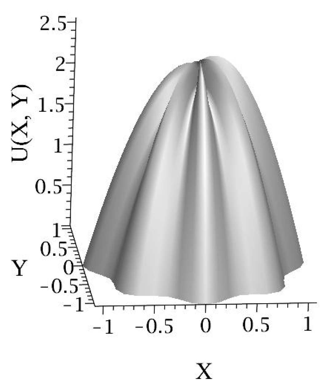
  • The Galerkin-based integral method assisted by symbolic manipulation software is an effective tool for investigating the fully developed laminar flow fluid in a corrugated cross-section cylindrical duct. Fully developed velocity profiles for any duct shape can be predicted by this method.
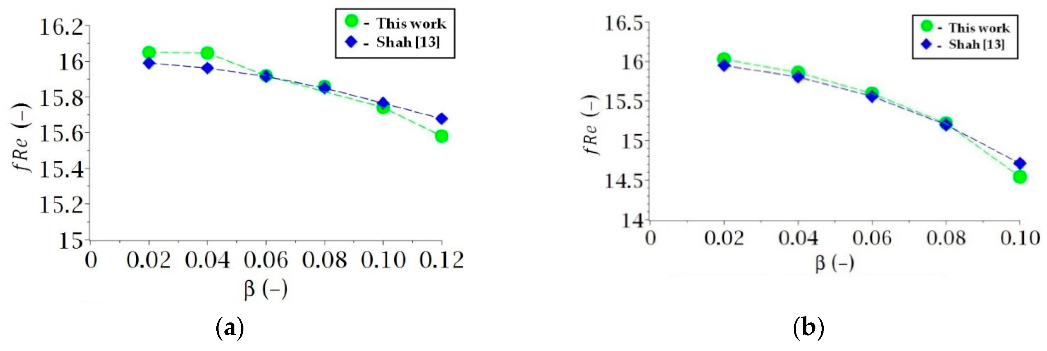
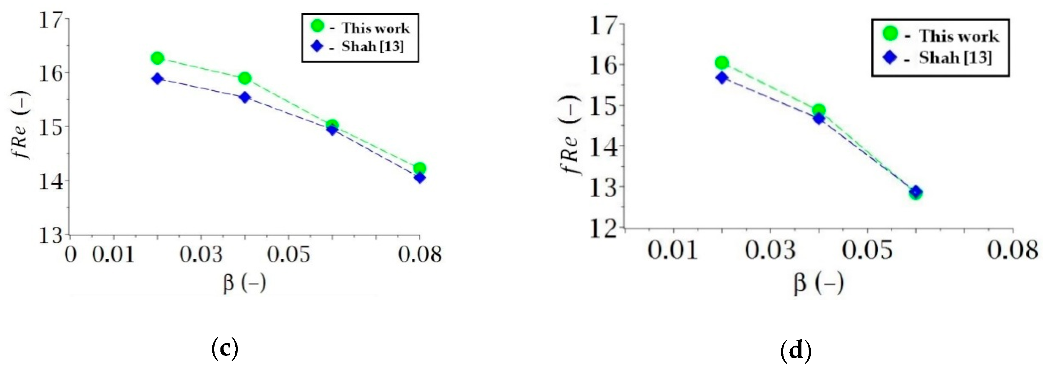
  • The Poiseuille number, f R e , obtained for different aspect ratios of the pipe was compared with the existing literature, and a good concordance was obtained in all studied cases.
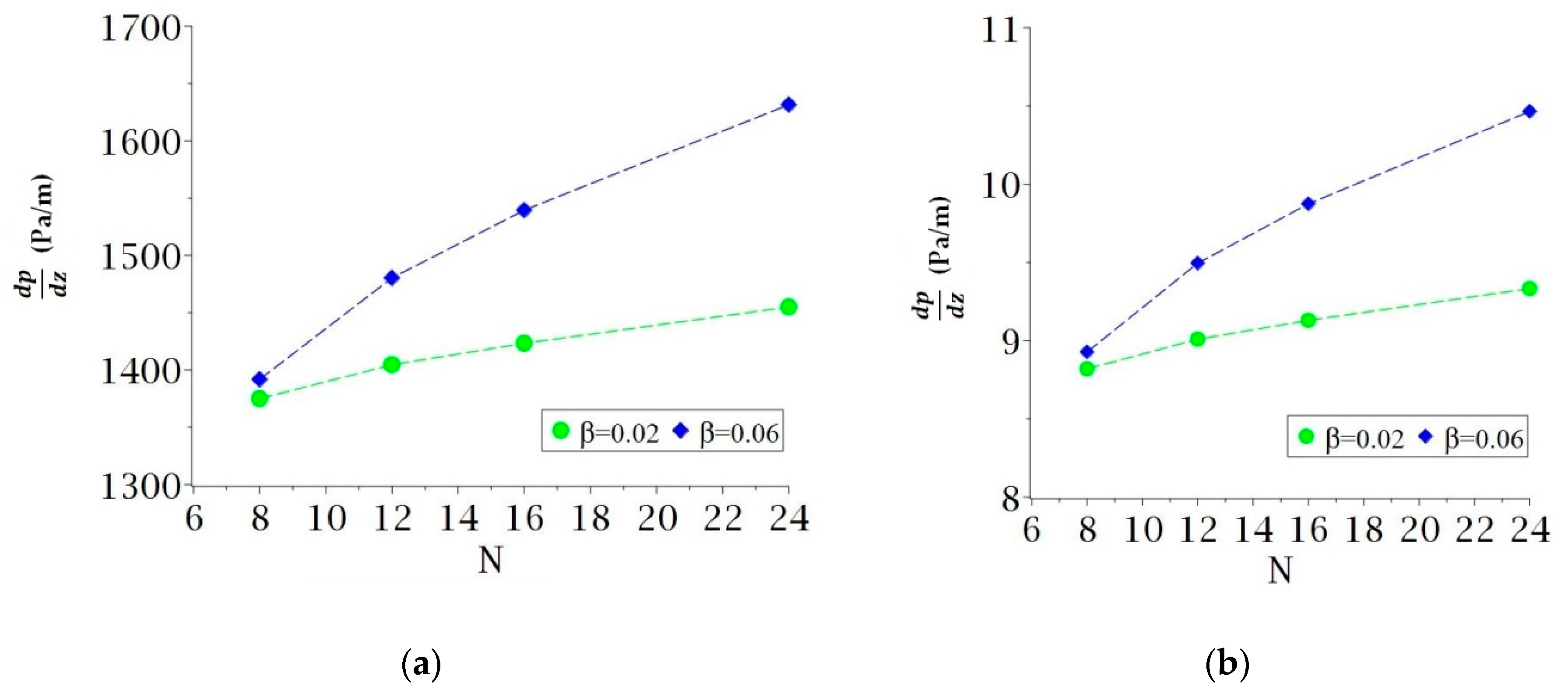
  • The appropriate number of base functions is different depending on the aspect ratio and the number of corrugations of the studied geometry. Such variation altered the computational time significantly. The smaller the number of base functions, the lower the computational time.
  • The pressure gradient increases with the number of corrugations and the aspect ratio of the pipe and decreases with the increase in the fluid temperature.
  • Values for the Reynolds number, Fanning friction factor, shear stress, and pressure gradient for heavy oil flow, with temperature-dependent viscosity, were presented. These results make it possible to better understand the behavior of heavy oil in corrugated cross-section ducts.

Author Contributions

Conceptualization, software, and formal analysis, V.A.d.S.J. and S.R.d.F.N.; writing—original draft preparation and editing, V.A.d.S.J.; supervision, review and resources, S.R.d.F.N. and A.G.B.d.L.; validation, formal analysis, review and funding acquisition, I.B.G., I.F.G., C.M.R.F. and J.E.F.d.C. All authors have read and agreed to the published version of the manuscript.

Acknowledgments

The authors thank CNPq, Finep, and Capes (Brazilian Research Agencies) for the financial support, and the authors of the cited references who helped in the improvement.

Conflicts of Interest

The authors declare no conflict of interest.

List of Symbols

a ,   b Geometric dimensions (m)
a i j Element of matrix A
A c Cross-section area of the duct (m2)
A 1 Inverse matrix of A
A ,   B ,   D Matrix
b j Element of matrix B (constants)
d h Hydraulic diameter (m)
d j Constants to be evaluated (constants)
D h Dimensionless hydraulic diameter
f   Fanning friction factor (dimensionless)
f i Base functions; Galerkin functions
f R e Poiseuille number (dimensionless)
L Characteristic length (m)
n Number of base functions
N u H 1 Nusselt number for the constant flux boundary condition
P Perimeter (m)
p Pressure (Pa)
r ,   θ ,   z Cylindrical coordinates
R e Reynolds number [dimensionless]
u Local axial velocity (m/s)
T Temperature (°C)
u m Mean velocity (m/s)
U Normalized velocity (dimensionless)
x ,   y ,   z Cartesian coordinates (m/s)
X ,   Y ,   Z Dimensionless coordinates (dimensionless)
W Dimensionless velocity (dimensionless)
W m Dimensionless mean velocity (dimensionless)
β Aspect ratio (dimensionless)
μ Dynamic viscosity (Pa·s)
ν Kinematic viscosity (cS)
ρ Density (kg/m3)
τ w   Shear stress (Pa)
Γ Boundary of duct
2 Laplacian operator

Abbreviations

GBIGalerkin-based integral

References

  1. Jadidi, A.; Saleh, S.J. Lubricated Transport of Heavy Oil Investigated by CFD. Ph.D. Thesis, Department of Engineering, University of Leicester, Leicester, UK, 2017. [Google Scholar]
  2. Andrade, T.H.F.; Damacena, Y.T.; Crivelaro, K.C.O.; Farias Neto, S.R.; Lima, A.G.B. Friction Reduction in Two-Phase Water-Oil Flow in Horizontal Tubes, XV Brazilian Congress of Mechanical Engineering; Águas de Lindóia: São Paulo, Brazil, 2010. (In Portuguese) [Google Scholar]
  3. Moharana, M.K.; Khandekar, S. Generalized formulation for estimating pressure drop in fully developed laminar flow in singly and doubly connected channels of non-circular cross-sections. Comput. Methods Appl. Mech. Eng. 2013, 259, 64–76. [Google Scholar] [CrossRef]
  4. Aparecido, J.B.; Cotta, R.M. Thermally developing laminar flow inside rectangular ducts. Int. J. Heat Mass Transf. 1990, 33, 341–347. [Google Scholar] [CrossRef]
  5. Syrjälä, S. Laminar flow of viscoelastic fluids in rectangular ducts with heat transfer: A finite element analysis. Int. Commun. Heat Mass Transf. 1998, 25, 191–204. [Google Scholar] [CrossRef]
  6. Aparecido, J.B.; Lindquist, C. Laminar Forced Convection through Rectangular Ducts with Uniform Axial and Peripheral Heat Flux; Brazilian Congress of Mechanical Engineering: Águas de Lindóia, Brazil, 1999. [Google Scholar]
  7. Lee, Y.M.; Kuo, Y.M. Laminar flow in annuli ducts with constant wall temperature. Int. Commun. Heat Mass Transf. 1998, 25, 227–236. [Google Scholar] [CrossRef]
  8. Venegas Prada, J.W. Experimental Study of Annular Oil-Water Flow (Core Flow) in the Elevation of Ultra-Hazardous Oils. Master’s Thesis, Petroleum Sciences, and Engineering, State University of Campinas, Campinas, Brazil, 1999. (In Portuguese). [Google Scholar]
  9. Bensakhria, A.; Peysson, Y.; Antonini, G. Experimental study of the pipeline lubrication for heavy oil transport. Oil Gas Sci. Technol. 2004, 59, 523–533. [Google Scholar] [CrossRef]
  10. Casarella, M.J.; Laura, P.A.; Chi, M. On the approximate solution of flow and heat transfer through non-circular conduits with uniform wall temperature. Br. J. Appl. Phys. 1967, 18, 1327. [Google Scholar] [CrossRef]
  11. Hu, M.H.; Chang, Y.P. Optimization of finned tubes for heat transfer in laminar flow. J. Heat Transf. 1973, 95, 332–338. [Google Scholar] [CrossRef]
  12. Shah, R.K. Laminar flow friction and forced convection heat transfer in ducts of arbitrary geometry. Int. J. Heat Mass Transf. 1975, 18, 849–862. [Google Scholar] [CrossRef]
  13. Courant, R.; David, H. Methods of Mathematical Physics: Partial Differential Equations; John Wiley & Sons: New York, NY, USA, 2008. [Google Scholar]
  14. Petrovsky, I.G. Lectures on Partial Differential Equations; Dover Publications: New York, NY, USA, 1991. [Google Scholar]
  15. Browder, F.E. Problemes Non-Lineaires; Presses de l’Université de Montréal: Montréal, QC, Canada, 1966; Volume 15. [Google Scholar]
  16. Dautray, R.; Lions, J.L. Mathematical Analysis and Numerical Methods for Science and Technology; Evolution Problems II; Springer Science & Business Media: Berlin/Heidelberg, Germany, 2012; Volume 6. [Google Scholar]
  17. Assan, A.E. Finite Elements Methods-First Steps; Unicamp: Campinas, Brazil, 2003. [Google Scholar]
  18. Cooper, J.M. Introduction to Partial Differential Equations with MATLAB; Springer Science & Business Media: Berlin/Heidelberg, Germany, 2012. [Google Scholar]
  19. Thomas, J.E. Fundamentals of Petroleum Engineering, 2nd ed.; Interciência, Petrobras: Rio de Janeiro, Brazil, 2004. (In Portuguese) [Google Scholar]
  20. Franco, C.M.R.; Barbosa de Lima, A.G.; Silva, J.V.; Nunes, A.G. Applying liquid diffusion model for continuous drying of rough rice in fixed bed. Defect Diffus. Forum 2016, 369, 152–156. [Google Scholar] [CrossRef]
  21. Santos, J.P.S.; Santos, I.B.; Pereira, E.M.A.; Silva, J.V.; de Lima, A.G.B. Wheat convective drying: An analytical investigation via galerkin-based integral method. Defect Diffus. Forum 2015, 365, 82–87. [Google Scholar] [CrossRef]
  22. Haji-Sheikh, A.; Mashena, M.; Haji-Sheikh, M.J. Heat transfer coefficient in ducts with constant wall temperature. J. Heat Transf. 1983, 105, 878–883. [Google Scholar] [CrossRef]
  23. Lakshminarayanan, R.; Haji-Sheikh, A. Entrance heat transfer in isosceles and right triangular ducts. J. Thermophys. Heat Transf. 1992, 6, 167–171. [Google Scholar] [CrossRef]
  24. Lee, Y.M.; Lee, P.C. Laminar flow in elliptic ducts with and without central circular cores for constant wall temperature. Int. Commun. Heat Mass Transf. 2001, 28, 1115–1124. [Google Scholar] [CrossRef]
Figure 1. (a) Aspect ratio in a corrugated duct; (b) sine-type corrugated duct.
Energies 13 01363 g001
Figure 2. Cross sections of the duct for different numbers of corrugations: (a) N = 8 ; (b) N = 12 ; (c) N = 16 ; (d) N = 24 .
Energies 13 01363 g002
Figure 3. Approximation in series of the function r ( θ ) .
Energies 13 01363 g003
Figure 4. Dimensionless velocity profile (surface curve; β = 0.08 and N = 8 ).
Energies 13 01363 g004
Figure 5. Data of f R e for different aspect ratios ( β ) of the pipe. (a) N = 8 ; (b) N = 12 ; (c) N = 16 ; (d) N = 24 .
Energies 13 01363 g005aEnergies 13 01363 g005b
Figure 6. The pressure gradient is a function of the number of corrugations for different aspect ratios and fluid temperatures: (a) T = 29.22 °C; (b) T = 260.3 °C.
Energies 13 01363 g006
Table 1. Values for temperature-dependent kinematic viscosity.
Oil
T °C ν (cS)
29.22180.21
51.1670.786
81.1125.526
108.511.840
137.96.3270
155.54.4980
199.62.3870
228.51.6520
260.31.1560
Table 2. Values for Poiseuille number, ( f R e ) , for a different number of corrugations.
N β This WorkRef [13] N β This WorkRef [13]
8 0.0216.04915.990160.0216.26915.887
0.0416.04615.962 0.0415.89415.542
0.0615.91815.915 0.0615.01514.943
0.0815.85815.850 0.0814.218 14.051
0.1015.74115.765
0.1215.57915.678
120.0216.02915.952240.0216.04315.679
0.0415.86015.806 0.0414.86814.671
0.0615.595 15.559 0.0612.83912.872
0.0815.216 15.200
0.1014.54114.711
Table 3. Values for the number of base functions chosen for each aspect ratio β .
N β n N β n
80.0212160.0212
0.0413 0.0415
0.0611 0.0615
0.087 0.085
0.105
0.125
120.0230240.0215
0.0452 0.0415
0.0610 0.06 6
0.0811
0.1010
Table 4. Values of the fluid dynamic parameter obtained in the simulations with β = 0.02 and N = 8 .
T
(°C)
μ
(Pa·s)
R e
(-)
f
(-)
τ ¯ w
(Pa)
d p d z
(Pa/m)
29.22171.60 11.0295 1.4413 686.20 1374.98
51.1767.400 28.0809 0.5661 269.52 540.061
81.1124.30577.8710 0.2041 97.192 194.750
108.511.273 167.883 0.0946 45.082 90.3333
137.9 6.0244 314.167 0.0506 24.090 48.2718
155.54.2828 441.9150.0359 17.126 34.3175
199.62.2728832.734 0.0190 9.0887 18.2116
228.51.5729 1203.23 0.0132 6.2901 12.6039
260.31.1007 1719.49 0.0092 4.4015 8.81970
Table 5. Values of the fluid dynamic parameters obtained in the simulations with β = 0.02 and   N = 12 .
T
(°C)
μ
(Pa·s)
R e
(-)
f
(-)
τ ¯ w
(Pa)
d p d z
(Pa/m)
29.22171.6010.94381.4341682.771404.52
51.1667.40027.86270.5632268.17 551.666
81.1124.305 77.26610.203196.707 198.935
108.511.273166.5790.094244.856 92.2744
137.96.0244311.7260.050323.97049.3091
155.54.2828438.4820.035717.04135.0549
199.62.2728826.2650.01899.043318.6029
228.51.57291193.880.01316.258712.8747
260.31.10071706.13 0.00914.37959.00922
Table 6. Values of the fluid dynamic parameters obtained in the simulations with β = 0.02 and     N = 16 .
T
(°C)
μ
(Pa·s)
R e
(-)
f
(-)
τ ¯ w
(Pa)
d p d z
(Pa/m)
29.2229.22 10.82772 1.4482689.491423.29
51.1651.16 27.56704 0.5688270.81559.040
81.1181.11 76.44601 0.205197.658201.594
108.5108.5 164.8108 0.095145.29893.5076
137.9137.9 308.4180 0.050824.20649.9681
155.5155.5 433.82850.036117.20835.5234
199.6199.6817.49510.01919.132318.8515
228.5228.51181.2110.01326.320313.0468
260.3260.31688.0280.00924.4226 9.12963
Table 7. Values of the fluid dynamic parameters obtained in the simulations with β = 0.02 and   N = 24 .
T
(°C)
μ
(Pa·s)
R e
(-)
f
(-)
τ ¯ w
(Pa)
d p d z
(Pa/m)
29.22171.6010.51788 1.4104671.50 1454.98
51.1667.40026.77820 0.5539263.75 571.485
81.1124.30574.25849 0.199795.110 206.082
108.511.273160.0947 0.092644.116 95.5893
137.96.0244299.5925 0.049523.57451.0805
155.54.2828421.4144 0.035216.75936.3142
199.62.2728794.1023 0.01868.894019.2712
228.51.57291147.410 0.01296.155313.3372
260.31.1007 1147.410 0.00904.30729.33287
Table 8. Values of the fluid dynamic parameters obtained in the simulations with β = 0.06 and N = 8 .
T
(°C)
μ
(Pa·s)
R e
(-)
f
(-)
τ ¯ w
(Pa)
d p d z
(Pa/m)
29.22171.6010.53431.3965664.891391.80
51.1667.40026.82000.5485261.15546.670
81.1124.30574.37450.197894.174197.133
108.511.273160.3440.091743.68291.4386
137.96.0244300.0600.049023.34248.8625
155.54.2828422.0720.034816.59434.7374
199.62.2728795.3420.01848.806518.4344
228.51.57291149.200.01286.094812.7581
260.31.10071642.28 0.00894.26498.92762
Table 9. Values of the fluid dynamic parameters obtained in the simulations with β = 0.06 and   N = 12 .
T
(°C)
μ
(Pa·s)
R e
(-)
f
(-)
τ ¯ w
(Pa)
d p d z
(Pa/m)
29.22 171.609.933301.3399637.911480.35
51.1667.40025.28980.5262250.55581.447
81.1124.30570.13120.189790.353209.674
108.511.273151.1960.088041.90997.2556
137.96.0244282.9410.047022.39551.9710
155.54.2828397.9920.033415.92136.9473
199.62.2728749.9660.01778.449119.6072
228.51.57291083.630.01225.847513.5697
260.31.10071548.580.00854.09189.49557
Table 10. Values of the fluid dynamic parameters obtained in the simulations with β = 0.06 and N = 16 .
T
(°C)
μ
(Pa·s)
R e
(-)
f
(-)
τ ¯ w
(Pa)
d p d z
(Pa/m)
29.22171.609.256481.2723605.761539.44
51.1667.40023.56670.4997237.92604.658
81.1124.30565.35270.180285.799218.044
108.511.273140.8940.083039.797101.138
137.96.0244263.6620.044021.26654.0456
155.54.2828370.8740.031015.11838.4222
199.62.2728698.8660.01688.023320.3899
228.51.57291009.800.01165.552714.1114
260.31.10071443.07 0.00813.88569.87463
Table 11. Values of the fluid dynamic parameters obtained in the simulations with β = 0.06 and N = 24 .
T
(°C)
μ
(Pa·s)
R e
(-)
f
(-)
τ ¯ w
(Pa)
d p d z
(Pa/m)
29.22171.60 7.926141.1217534.0361631.59
51.1667.40020.17970.4405209.757640.854
81.1124.30555.96030.158875.6402231.097
108.511.273120.6450.073635.0850107.192
137.96.0244225.7690.039318.748557.28089
155.54.2828317.5720.027913.328740.7222
199.62.2728598.4250.01487.0733021.6104
228.51.5729864.6740.01024.8953014.9562
260.31.10071235.670.00713.4255310.4657

