A New Simulation Model for Vertical Spiral Ground Heat Exchangers Combining Cylindrical Source Model and Capacity Resistance Model

 ,
,  ,
, 
Abstract
:
1. Introduction
2. Calculation Method for Vertical Spiral Ground Heat Exchangers
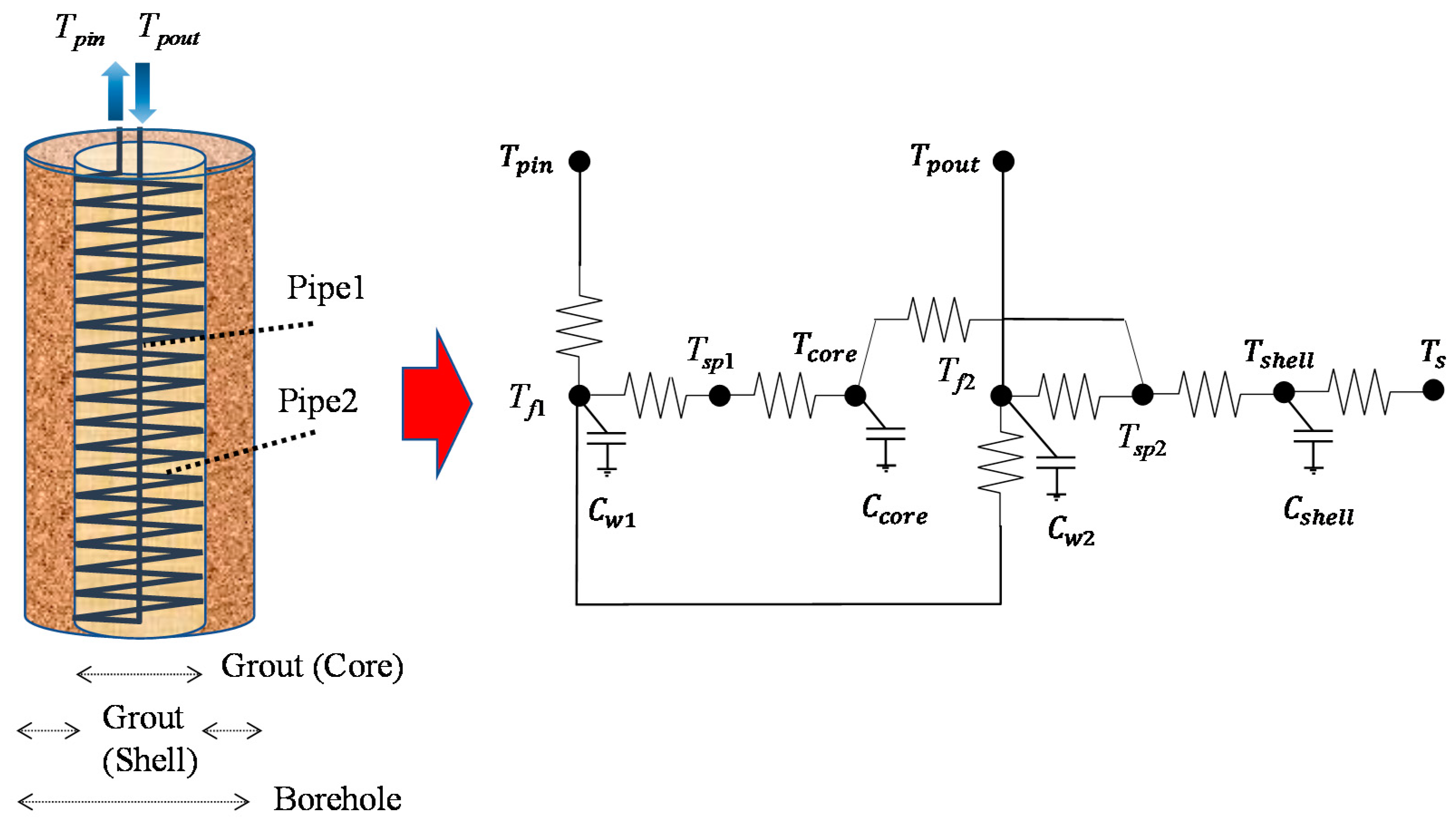
2.1. Calculation Method for Inside Spiral Ground Heat Exchangers
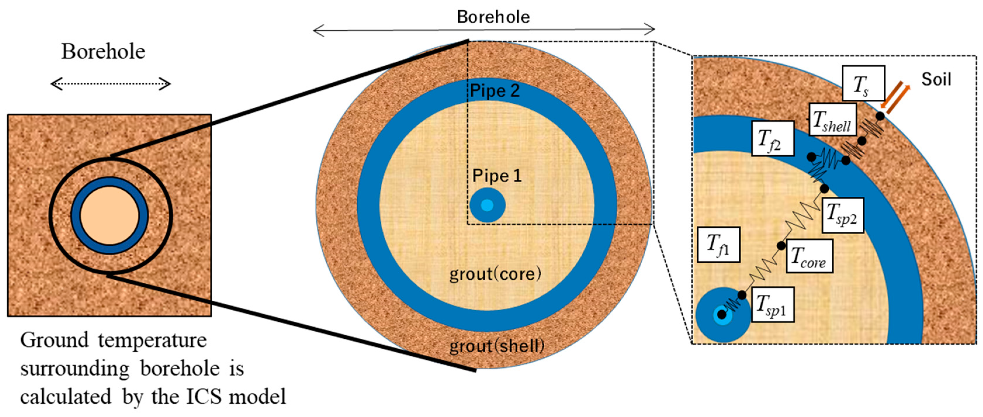
2.2. Calculation Method for Underground Temperature
2.3. Calculation Method for Ground Source Heat Pump System
3. Validation of Simulation Model by Comparing with Measurement Data
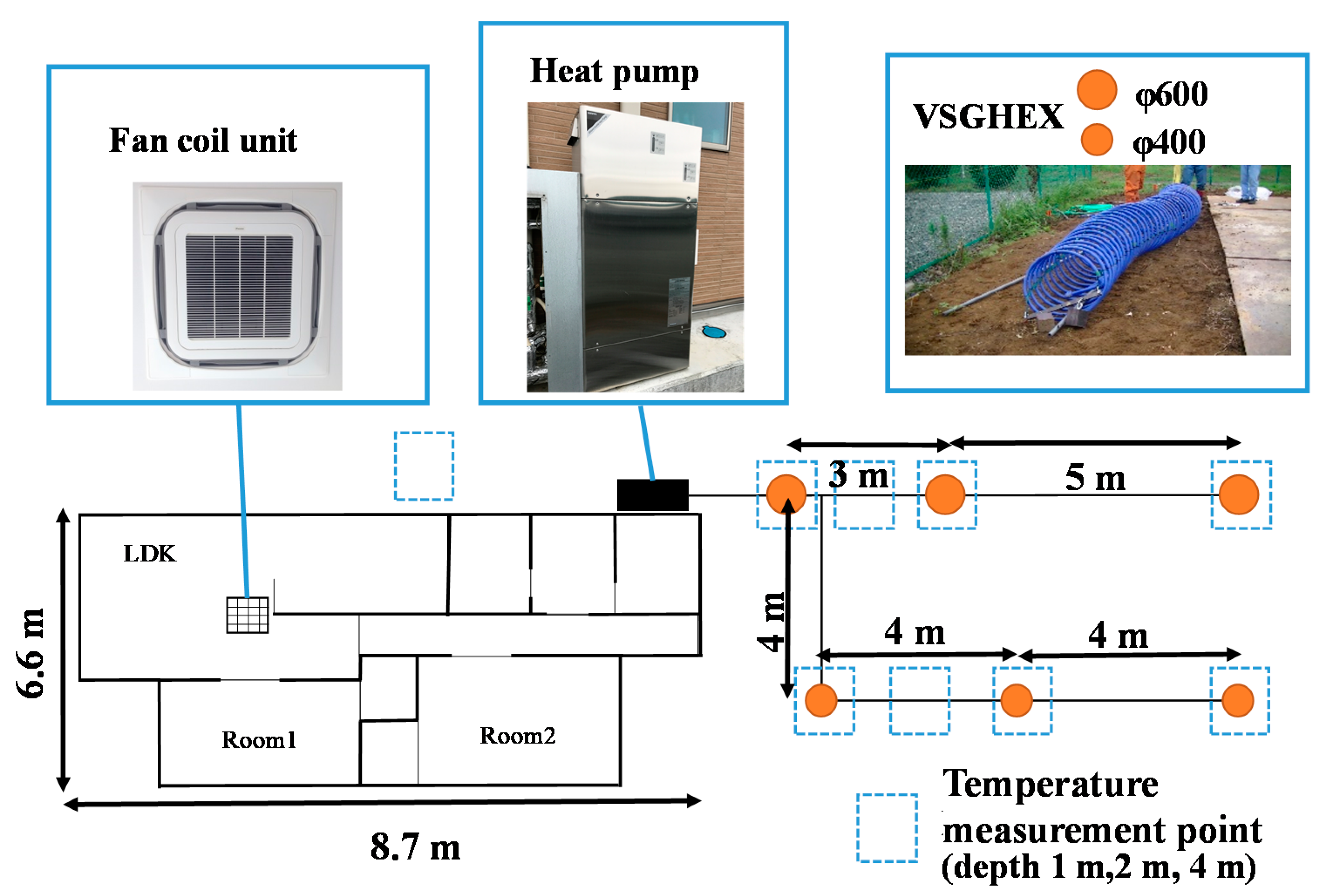
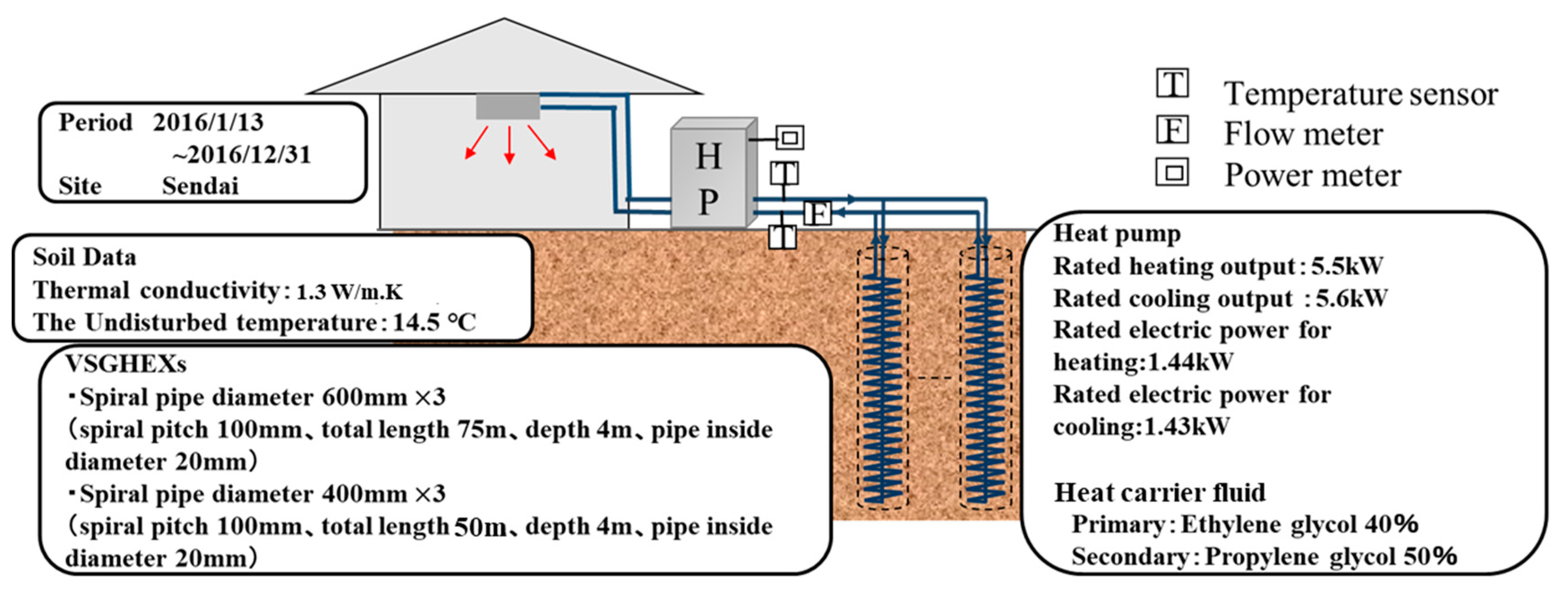
3.1. Outlines of Measurement
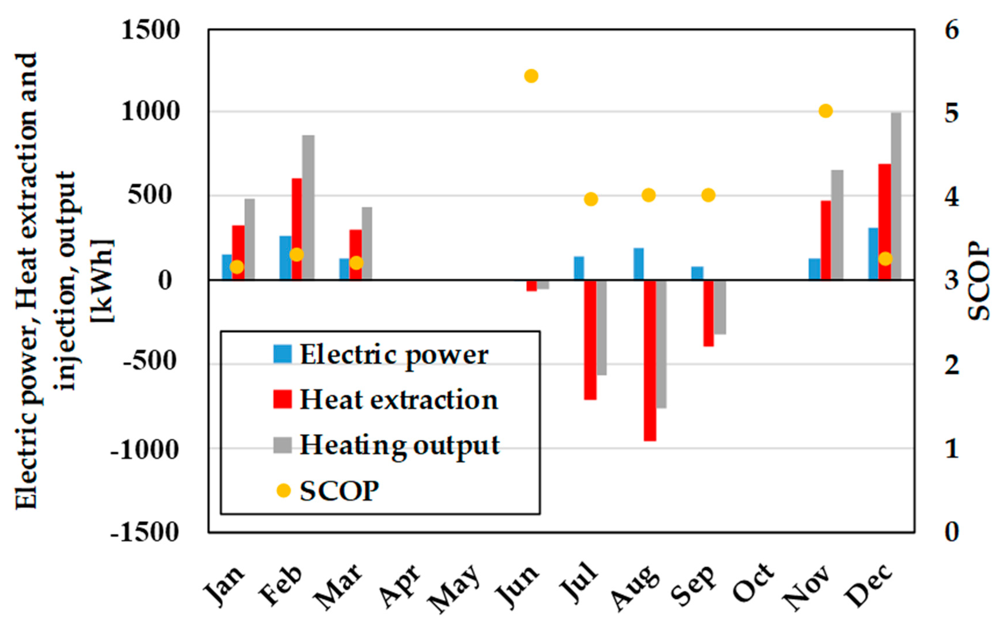
3.2. Result of Measurement
3.3. Validation of Calculation
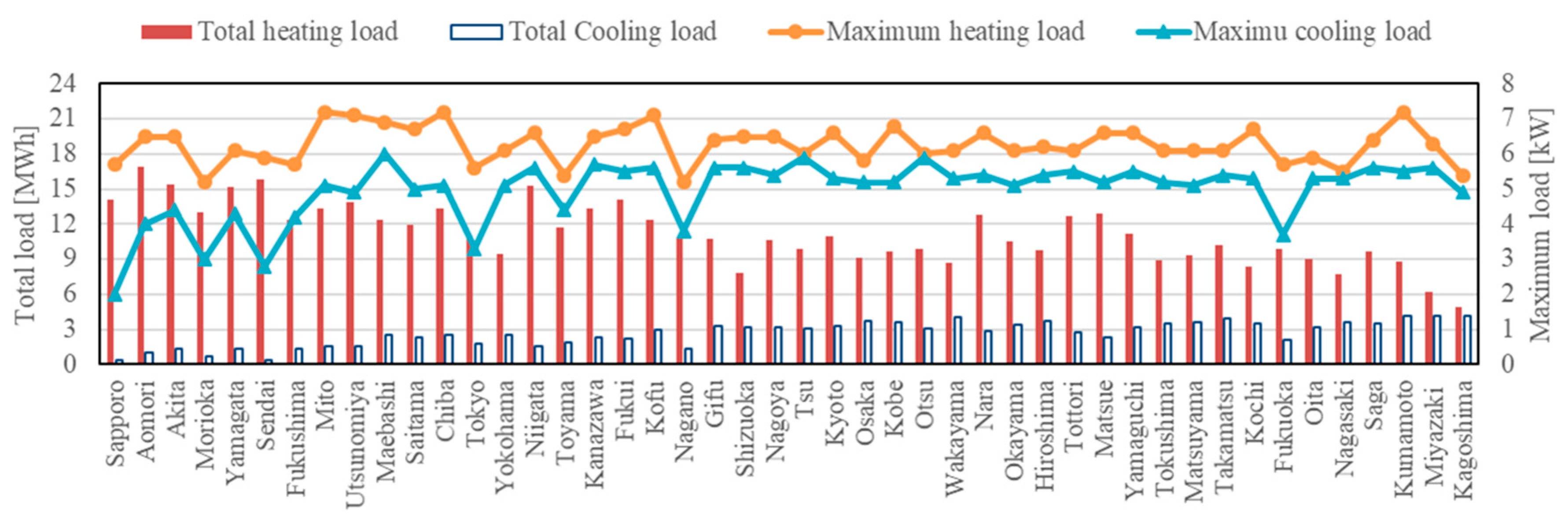
4. Estimation of Number of Vertical Spiral Ground Heat Exchangers for a Residential House
Calculation Conditions
5. Result and Discussion
6. Conclusions
- (1)
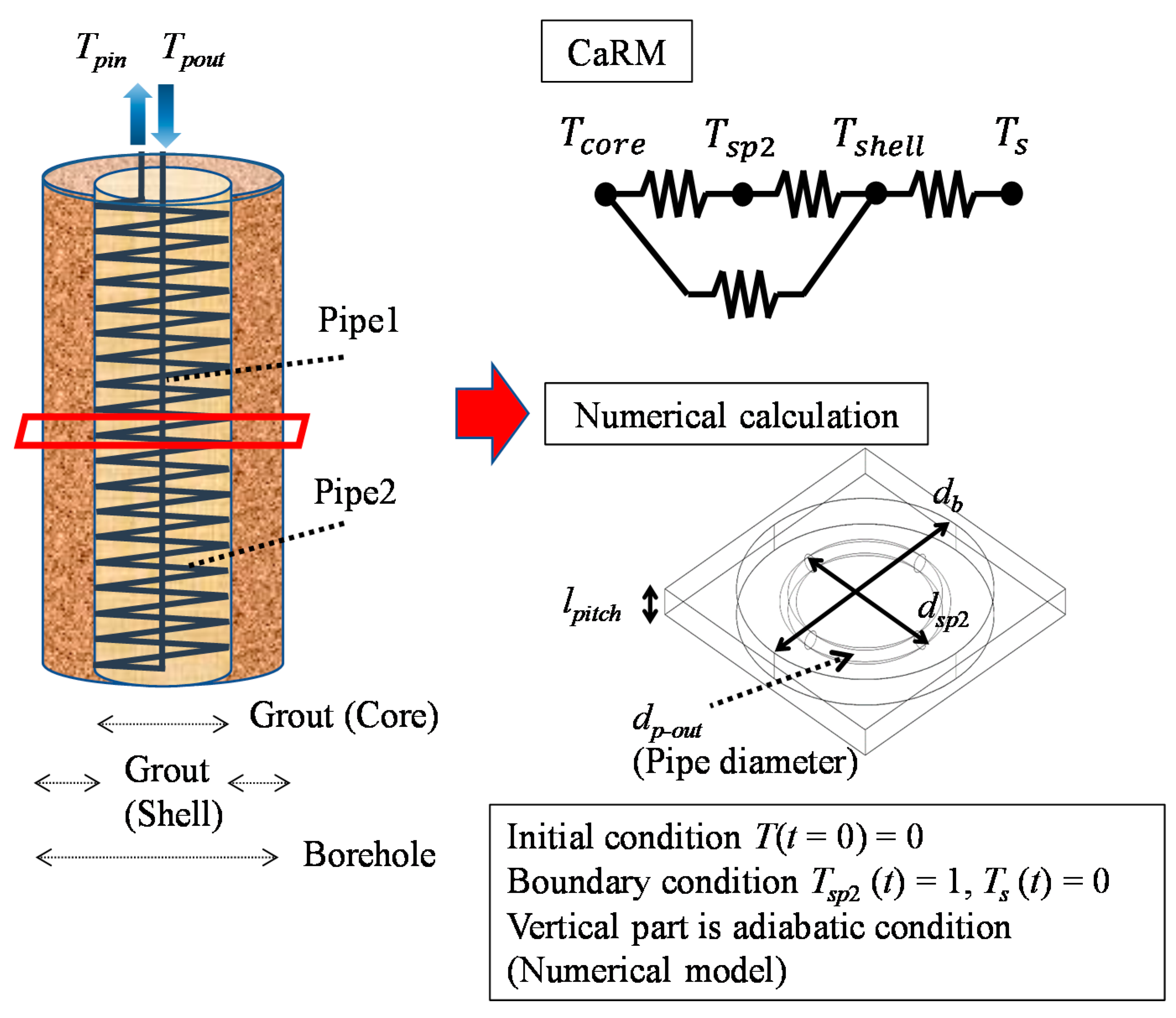
- A new simulation model for VSGHEXs was developed by combining the ICS model with the CaRM. In this model, the ground temperature surrounding VSGHEX can be calculated by applying the ICS model and the temperatures inside VSGHEX are calculated by CaRM. The developed simulation model can consider the heat capacity inside VSGHEX and provide dynamic calculation with high speed and appropriate precision.
- (2)
- In order to apply the CaRM, the equivalent length was introduced. Then, the equivalent length was approximated by comparing the results of CaRM and the numerical calculation. As the result, the relative error of heat transmission (thermal resistance) at steady sate between the numerical calculation and the developed method (Applying the CaRM and equivalent length) was 2.1% at the maximum.
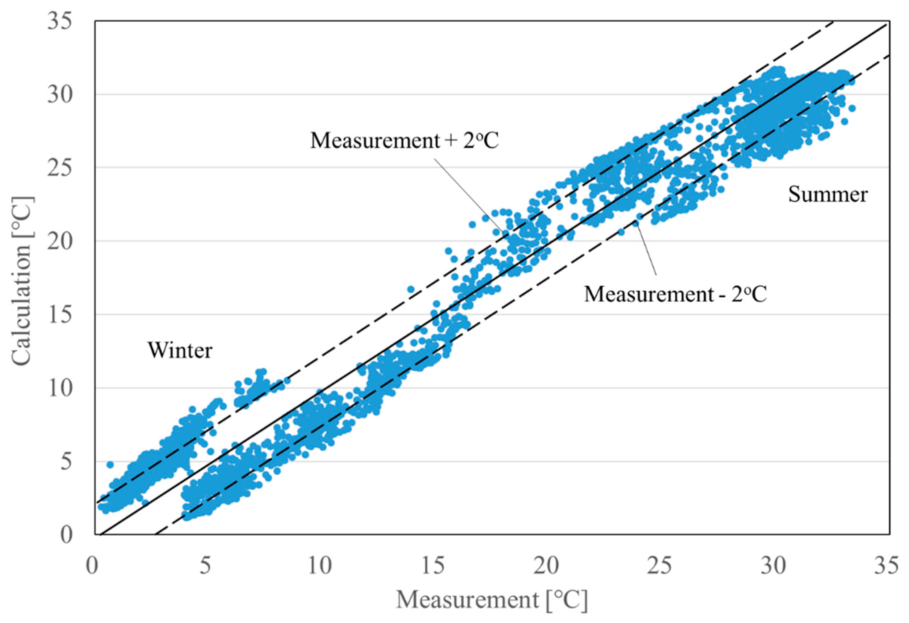
- (3)
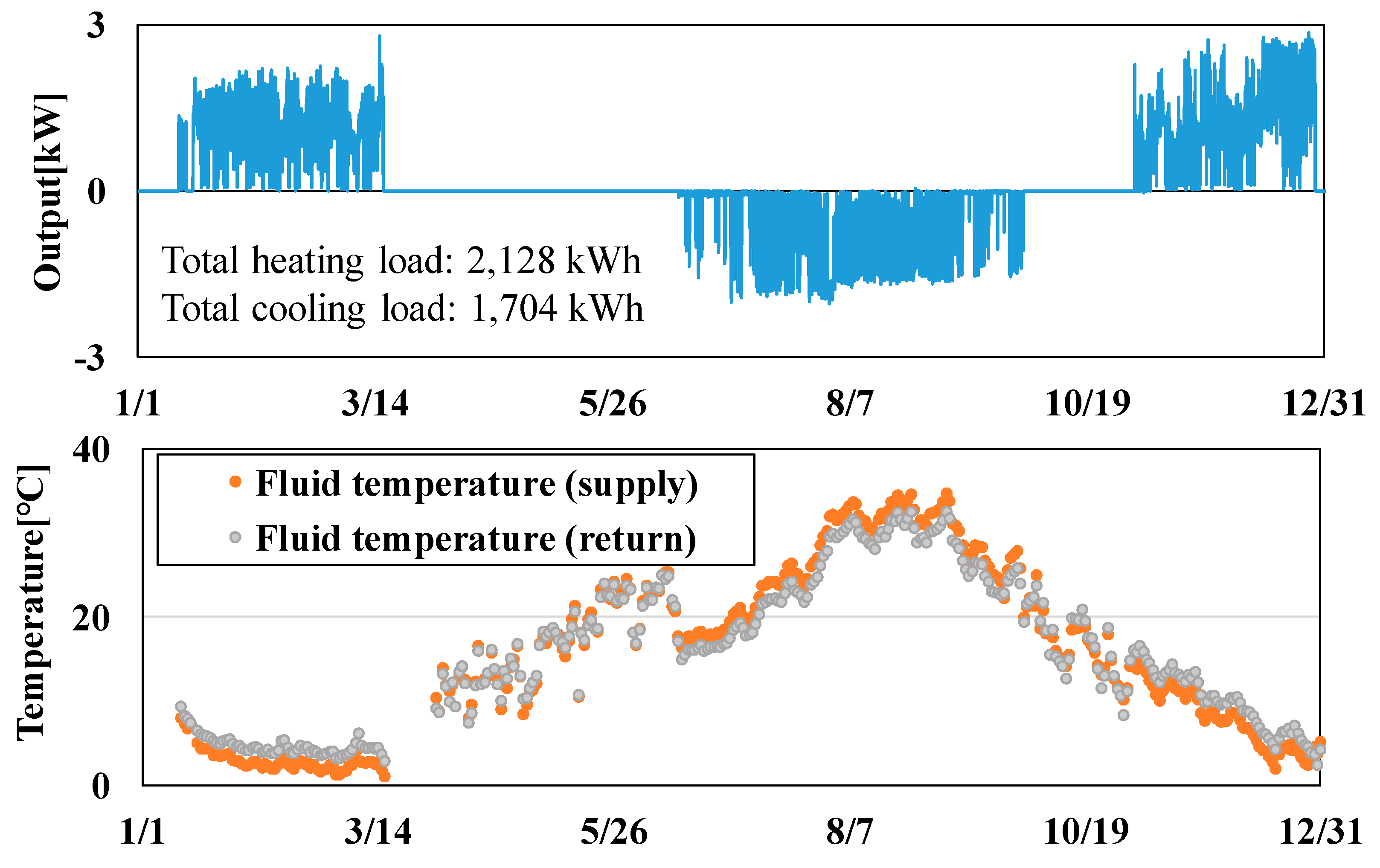
- The calculation model of the VSGHEX was integrated into the design and simulation tool for the GSHP system. The accuracy of the tool was verified by comparing with the measurements. The error between supply temperatures of the measurements and calculation is approximately 2 °C at the maximum annually. It can be said that the calculated temperature reproduces the measured one with appropriate accuracy.
- (4)
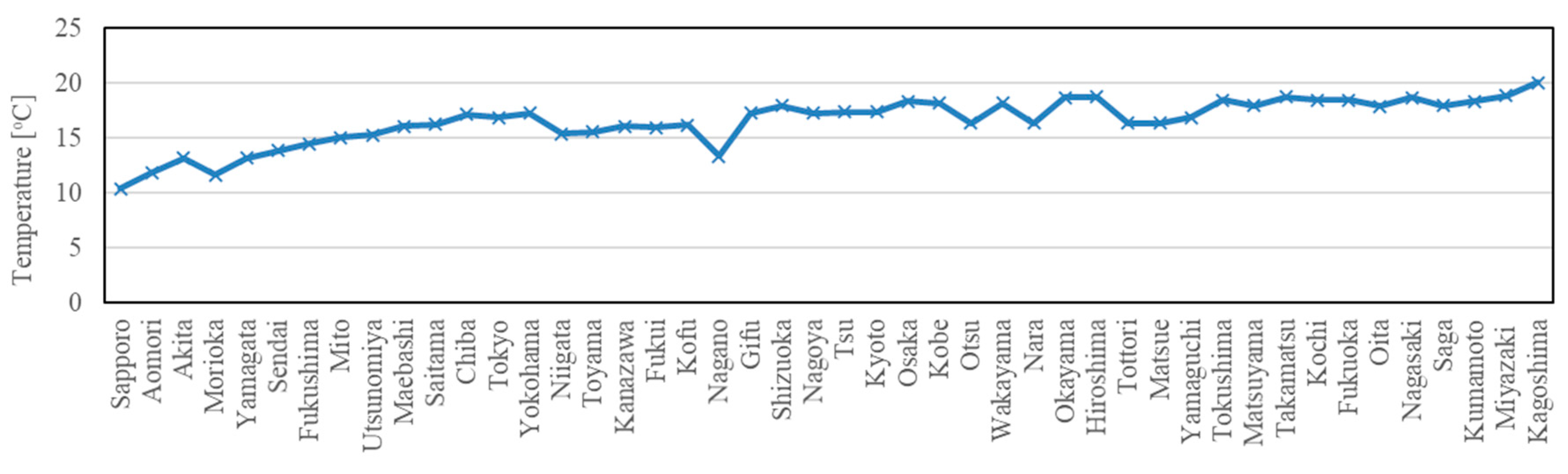
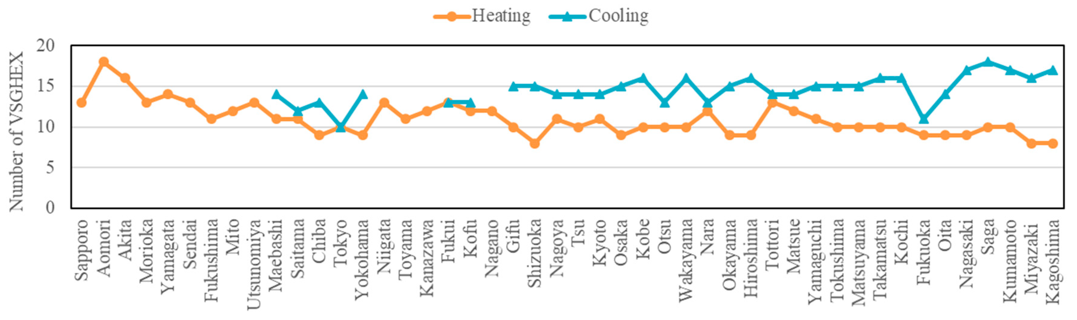
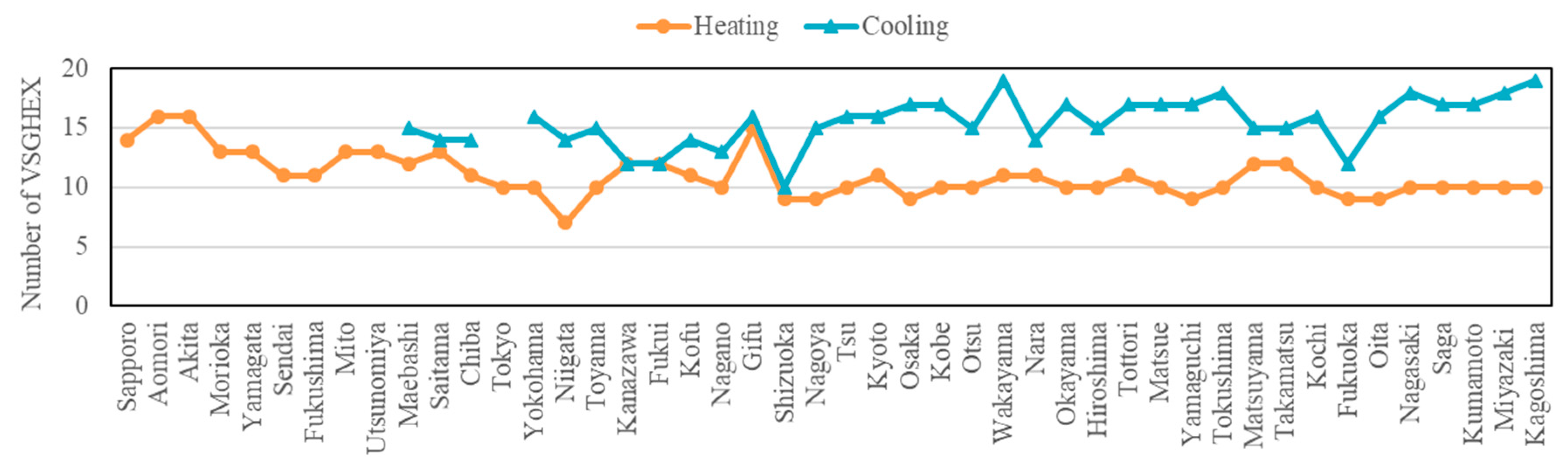
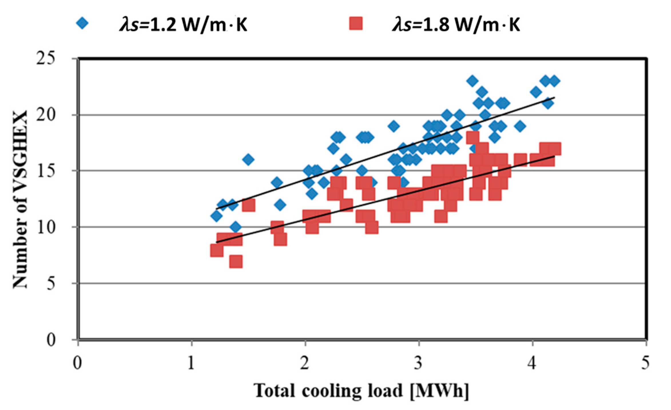
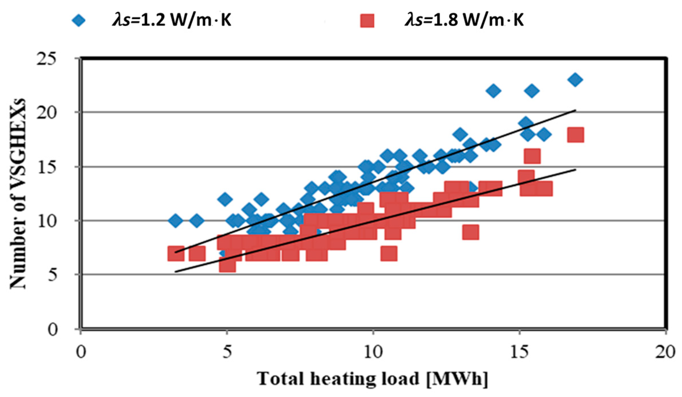
- Assuming the GSHP system with VSGHEXs, whose spiral diameter was 500 mm and depth was 4 m, was installed in the residential house in Japan, the required numbers of VSGHEXs were estimated. The results showed a strong correlation between the total heating or cooling load and the required number. Therefore, the required number can be regarded as the function of the total heating or cooling load, the effective thermal conductivity of soil, and the undisturbed ground temperature. Then, the required number can be estimated by using the simplified approximate equation.
Author Contributions
Funding
Acknowledgments
Conflicts of Interest
Nomenclature
| a | Thermal diffusivity (m2/s) |
| c | Specific heat (J/kg·K) |
| d | Diameter (m) |
| E | Electric power consumption of heat pump unit (W) |
| G | Flow rate (m3/s) |
| h | Convective heat transfer rate (W/m2·K) |
| Jx | xth-order Bessel function of first kind (-) |
| l | Length [m] |
| n | Number of time step (-) |
| q | Heat injection rate per length (W/m) |
| Q | Heat extraction, heat load (W) |
| r | Radius (m) |
| r* | Non-dimensional distance (-) |
| T | Temperature (°C) |
| t | Time (h) |
| t* | Non-dimensional time (Fourier number) (-) |
| T* | Non-dimensional temperature (-) |
| u | Characteristic value (-) |
| V | Volume (m3] |
| Yx | xth-order Bessel function of second kind (-) |
| λ | Thermal conductivity (W/m·K) |
| ρ | Density (kg/m3) |
| τ | Parameter relating to time (h) |
| τ* | Non-dimensional parameter relating to time (-) |
| Subscripts | |
| 1 | Heat pump primary side |
| 1f | Heat carrier fluid in the primary side |
| 1in | Inlet in the primary side |
| 1in | Outlet in the primary side |
| 2 | Heat pump secondary side |
| b | Borehole |
| C | Temperature response of ICS problem |
| c | Cooling |
| core | Core |
| d | Distance |
| f | Heat carrier fluid |
| f1 | Heat carrier fluid in Pipe1 |
| f1in | Heat carrier fluid at inlet of Pipe1 |
| f1out | Heat carrier fluid at outlet of Pipe1 |
| f2 | Heat carrier fluid in Pipe2 |
| f2in | Heat carrier fluid at inlet of Pipe2 |
| f2out | Heat carrier fluid at outlet of Pipe2 |
| g | Grout |
| h | Heating |
| l | Code number of approximate rectangular step load |
| n | Number of time step |
| p2 | Equivalent (length) |
| pin | Inlet of ground heat exchanger |
| p-in | Pipe inside |
| pitch | Pitch of spiral pipe |
| pout | Outlet of ground heat exchanger |
| p-out | Pipe outside |
| s | Soil |
| s0 | Soil initial |
| shell | Shell |
| sp1 | Surface of Pipe1 |
| sp2 | Spiral pipe (Pipe2), Surface of Pipe2 |
References
- Miyara, A. Thermal performance and pressure drop of spiral-tube ground heat exchangers for ground-source heat pump. Appl. Therm. Eng. 2015, 90, 630–637. [Google Scholar]
- Dehghan, B. Experimental and computational investigation of the spiral ground heat exchangers for ground source heat pump applications. Appl. Therm. Eng. 2017, 121, 908–921. [Google Scholar] [CrossRef]
- Li, H.; Nagano, K.; Lai, Y. A new model and solutions for a spiral heat exchanger and its experimental validation. Int. J. Heat Mass Transf. 2012, 55, 4404–4414. [Google Scholar] [CrossRef]
- Li, H.; Nagano, K.; Lai, Y. Heat transfer of a horizontal spiral heat exchanger under groundwater advection. Int. J. Heat Mass Transf. 2012, 55, 6819–6831. [Google Scholar] [CrossRef]
- Go, G.H.; Lee, S.R.; Yoon, S.; Kang, H.B. Design of spiral coil PHC energy pile considering effective borehole thermal resistance and groundwater advection effects. Appl. Energy 2014, 125, 165–178. [Google Scholar] [CrossRef]
- Zhang, W.; Yang, H.; Lu, L.; Cui, P.; Fang, Z. The research on ring-coil heat transfer models of pile foundation ground heat exchangers in the case of groundwater seepage. Energy Build. 2014, 71, 115–128. [Google Scholar] [CrossRef]
- Li, M.; Lai, A.C. Heat-source solutions to heat conduction in anisotropic media with application to pile and borehole ground heat exchangers. Appl. Energy 2012, 96, 451–458. [Google Scholar] [CrossRef]
- Zarrella, A.; De Carli, M. Heat transfer analysis of short helical borehole heat exchangers. Appl. Energy 2013, 102, 1477–1491. [Google Scholar] [CrossRef]
- Zarrella, A.; Capozza, A.; De Carli, M. Performance analysis of short helical borehole heat exchangers via integrated modelling of a borefield and a heat pump: A case study. Appl. Therm. Eng. 2013, 61, 36–47. [Google Scholar] [CrossRef]
- Zarrella, A.; De Carli, M.; Galgaro, A. Thermal performance of two types of energy foundation pile: Helical pipe and triple U-tube. Appl. Therm. Eng. 2013, 61, 301–310. [Google Scholar] [CrossRef]
- Zarrella, A.; Emmi, G.; De Carli, M. Analysis of operating modes of a ground source heat pump with short helical heat exchangers. Energy Convers. Manag. 2015, 97, 351–361. [Google Scholar] [CrossRef]
- Nagano, K.; Katsura, T.; Takeda, S. Development of a design and performance prediction tool for the ground source heat pump system. Appl. Therm. Eng. 2006, 26, 1578–1592. [Google Scholar] [CrossRef]
- Carslaw, H.S.; Jaeger, J.C. Conduction of Heat in Solid; Oxford University Press: Oxford, UK, 1959. [Google Scholar]
- Deerman, J.D.; Kavanaugh, S.P. Simulation of Vertical U-tube Ground-coupled Heat Pump Systems Using the Cylindrical Heat Source Solution. ASHRAE Trans. 1990, 97, 287–295. [Google Scholar]
- Katsura, T.; Nagano, K.; Takeda, S. Method of calculation of the ground temperature for multiple ground heat exchangers. Appl. Therm. Eng. 2008, 28, 1995–2004. [Google Scholar] [CrossRef]
- Katsura, T.; Nagano, K.; Narita, S.; Takeda, S.; Nakamura, Y.; Okamoto, A. Calculation Algorithm of the Temperatures for Pipe Arrangement of Multiple Ground Heat Exchangers. Appl. Therm. Eng. 2009, 29, 906–919. [Google Scholar] [CrossRef]
- Katsura, T.; Nagano, K.; Sakata, Y.; Higashitani, T. A Design and Simulation Tool for Ground Source Heat Pump System and Borehole Thermal Storage System. In Proceedings of the 14th International Conference on Energy Storage EnerSTOCK2018, Adana, Turkey, 25–28 April 2018. [Google Scholar]
- Li, S.; Dong, K.; Wang, J.; Zhang, X. Long term coupled simulation for ground source heat pump and underground heat exchangers. Energy Build. 2015, 106, 13–22. [Google Scholar] [CrossRef]
- Architecture Environment Solutions: AE-CAD/AE-Simheat. Available online: http://www.ae-sol.co.jp/aesol01.html (accessed on 6 July 2018).


| Tube Diameter dp-out (m) | Borehole Diameter db (mm) | Spiral Pitch lpitch (mm) | Coefficient C | lp2 (mm) | |
|---|---|---|---|---|---|
| CASE1 | 16 | 450 | 60 | 0.771 | 37.8 |
| CASE2 | 16 | 450 | 35 | 0.762 | 24.6 |
| CASE3 | 16 | 450 | 140 | 0.693 | 57.6 |
| CASE4 | 16 | 800 | 60 | 0.824 | 42.1 |
| CASE5 | 16 | 800 | 35 | 0.832 | 27.3 |
| CASE6 | 16 | 800 | 140 | 0.734 | 65.4 |
| CASE7 | 20 | 450 | 140 | 0.672 | 58.9 |
| CASE8 | 25 | 450 | 140 | 0.640 | 58.7 |
| Numerical | CaRM | Relative Error (%) | |
|---|---|---|---|
| CASE1 | 14.06 | 13.86 | 1.4 |
| CASE2 | 15.11 | 15.34 | 1.5 |
| CASE3 | 10.58 | 10.50 | 0.8 |
| CASE4 | 15.84 | 15.60 | 1.5 |
| CASE5 | 16.93 | 16.94 | 0.1 |
| CASE6 | 12.04 | 12.29 | 2.1 |
| CASE7 | 11.31 | 11.24 | 0.6 |
| CASE8 | 12.15 | 12.18 | 0.2 |
| Year of completion | 2016/1 |
| Total floor area | 57 m2 |
| Floor | On-storied house |
| Q value | 2.92 W/m2·K |
| Period | Set Temperature (°C) | Area of AC (m2) |
|---|---|---|
| 13 Jan.–16 Mar. | 20 | 31 |
| Arbitrarily | 31 | |
| 15 Jun.–30 Sep. | 24 | 46 |
| Arbitrarily | 31 | |
| 1 Nov.–31 Dec. | 22 | 31 |
| Arbitrarily | 31 |
| Name of City | Q Value(W/m2 K) | |
|---|---|---|
| Next-Generation Energy Standard Value | High Insulated | |
| Sapporo | 1.6 | 1 |
| Morioka, Nagano | 1.9 | 1.3 |
| Aomori, Akita, Yamagata, Sendai, Fukushima, Toyama | 2.4 | 1.9 |
| Others | 2.7 | 2 |
© 2020 by the authors. Licensee MDPI, Basel, Switzerland. This article is an open access article distributed under the terms and conditions of the Creative Commons Attribution (CC BY) license (http://creativecommons.org/licenses/by/4.0/).
Share and Cite
Katsura, T.; Higashitani, T.; Fang, Y.; Sakata, Y.; Nagano, K.; Akai, H.; OE, M. A New Simulation Model for Vertical Spiral Ground Heat Exchangers Combining Cylindrical Source Model and Capacity Resistance Model. Energies 2020, 13, 1339. https://doi.org/10.3390/en13061339
Katsura T, Higashitani T, Fang Y, Sakata Y, Nagano K, Akai H, OE M. A New Simulation Model for Vertical Spiral Ground Heat Exchangers Combining Cylindrical Source Model and Capacity Resistance Model. Energies. 2020; 13(6):1339. https://doi.org/10.3390/en13061339
Chicago/Turabian StyleKatsura, Takao, Takashi Higashitani, Yuzhi Fang, Yoshitaka Sakata, Katsunori Nagano, Hitoshi Akai, and Motoaki OE. 2020. "A New Simulation Model for Vertical Spiral Ground Heat Exchangers Combining Cylindrical Source Model and Capacity Resistance Model" Energies 13, no. 6: 1339. https://doi.org/10.3390/en13061339
APA StyleKatsura, T., Higashitani, T., Fang, Y., Sakata, Y., Nagano, K., Akai, H., & OE, M. (2020). A New Simulation Model for Vertical Spiral Ground Heat Exchangers Combining Cylindrical Source Model and Capacity Resistance Model. Energies, 13(6), 1339. https://doi.org/10.3390/en13061339