Operational Simulation Environment for SCADA Integration of Renewable Resources

Abstract

The complexity of power systems is rising mainly due to the expansion of renewable energy generation. Due to the enormous variability and uncertainty associated with these types of resources, they require sophisticated planning tools so that they can be used appropriately. In this sense, several tools for the simulation of renewable energy assets have been proposed. However, they are traditionally focused on the simulation of the generation process, leaving the operation of these systems in the background. Conversely, more expert SCADA operators for the management of renewable power plants are required, but their training is not an easy task. SCADA operation is usually complex, due to the wide set of information available. In this sense, simulation or co-simulation tools can clearly help to reduce the learning curve and improve their skills. Therefore, this paper proposes a useful simulator based on a JavaScript engine that can be easily connected to any renewable SCADAs, making it possible to perform different simulated scenarios for novel operator training, as if it were a real facility. Using this tool, the administrators can easily program those scenarios allowing them to sort out the lack of support found in setting up facilities and training of novel operator tasks. Additionally, different renewable energy generation models that can be implemented in the proposed simulator are described. Later, as a use example of this tool, a study case is also performed. It proposes three different wind farm generation facility models, based on different turbine models: one with the essential generation turbine function obtained from the manufacturer curve, another with an empirical model using monotonic splines, and the last one adding the most important operational states, making it possible to demonstrate the usefulness of the proposed simulation tool.

1. Introduction

In the last few years, the presence of renewable energy sources has increased significantly within the power systems. These new sources, contrary to the traditional energy approach, are not only generated in huge central, but also in distributed small, mini, or micro power plants. This approach is covered under the paradigm called Distributed Generation (DG) [1]. Specifically, this paradigm is one of the keystones in Smart Grids (SG) [2,3,4,5], following an optimal control of all the connected elements, including in them an active role of consumers and producers and even proposing a new actor, the prosumer. In the DG paradigm, the resources of generation and/or storage are connected directly to the distribution network, as it is defined in the EU Directive 2019/944 [6]. In this way, they are located closer to consumption points. Those elements, which are usually renewables, are called Distributed Energy Resources (DERs) [7].

Taking under consideration these trends, it is clear that the power system is becoming more complex: the number of generation points is increasing, and the production is highly dependent on the weather. This is why different technologies are used in SG to achieve the monitoring and control levels to maintain the coordination and stability of the whole system. Those advances cover all the areas from Automatic Metering Infrastructure (AMI) [8], fault location systems [9], electric vehicle integration [10], and of course, the generation control. Above all, reliable systems for planning, coordination, and analysis are an imperative in the future of the power system.

Specifically, it is in generation control where prediction and simulation are especially important. The balancing of the whole power system depends on how accurate the predictions of generation are, an aspect that is becoming more and more difficult due to the increasing number of DG facilities.

In this sense, utilities or power companies are currently integrating, at different levels, tools to support their assets’ management. This trend is included in their strategies of network digitization, in which the digital twin is the paradigm that is arousing more interest [11]. Thus, thanks to the greater knowledge of the network that provides these technologies (more detailed models and greater amount of real-time data), it is possible to define new analytic applications and diagnosis based on this network characterization (e.g., [12,13]).

Specifically, simulation software is directly affected by this improvement of the network characterization. The ability to reproduce the behavior of a system in different scenarios or configurations is very useful, becoming essential tools for planning tasks. Due to this, it is easy to find simulators for the study, modeling, or design of DER elements.

On the one hand, there is software focused on the analysis or the design of the DER elements themselves. For example, QBlade is widely used to design blades and simulate their behavior, achieving good results even in cases of vortexes’ existence [14] or low wind conditions [15]. PVSyst^TM is a software tool to size photovoltaic (PV) facilities and to estimate their production depending on the geographic situation, solar panel technology, and other parameters [16]; likewise, Bluesol is a similar example [17].

On the other hand, general power simulators can be also used to study the DER behavior. Thus, this second group is usually divided into two types: Electromagnetic Transient (EMT) analysis and power flow analysis. In this first approach, EMT tools such as PSCAD^TM, DIgSILENT PowerFactory^TM, and the MATLAB^R SimPowerSystems^TM toolbox have been widely used through their model library to simulation of the transient behavior of individual assets or sets of them. As an example, PowerFactory^TM has been used in [18] to simulate the wind turbine model following the guidelines defined by the IEC 61400-27-1 [19]; or PSCAD^TM, which was used in [20] to test a new protection scheme for relay in power systems with PV generation; or in [21] to test dynamic reactive power compensations for PV inverters. MATLAB^® and Simulink^® have been also extensively used for the simulation of microgrids and hybrid systems using ad hoc models (e.g., [22]). In the second subgroup, power flow simulators are focusing on energy transfer and lose analysis along the power system. Simulation tools such as PowerWorld^TM, PSS^®E, and OpenDSS are commonly applied for this type of study, even being integrated into the corporate utilities’ tools. As an example, PowerWorld^TM was used in [23] to carry out a review of complex network analysis in electric power systems using an IEEE Node Test Feeder [24]. Besides, OpenDSS is a free software by EPRI^®, which has been used in Demand Response (DR) analyses [25], Volt-Var Optimization (VVO) [26], etc. Moreover, OpenDSS is also suitable for evaluating the analysis under different harmonic orders, making Power Quality (PQ)analyses possible (e.g., [27]). Furthermore, new tools like DRIVE [28] completes OpenDSS’s capabilities, making Hosting Capacity Analysis (HCA) possible [29], which is essential for utilities in the present scenario of DER deployment and the application in new flexibility services [30].

Thus, it is important to note that, when the simulation is applied considering cyber-physical systems, different components could be interconnected to form a more complete one. For example, for a PV farm simulation, not only is the model of the solar panels necessary, but also, the models of the inverters and the control system should be studied in order to create a more realistic and complete scenario. This approach in which different simulation models are combined is called co-simulation [31]. An example of a simulator that covers this function is Mosaik, a framework for SG co-simulation [32]. This tool has been used by researchers for the study and evaluation of different energy scenarios [33].

In summary, all of these tools are focused on: (A) the analysis or design of the elements or (B) studying DER energy production and power flow for planning task. As can be seen, it is not usual that they take under consideration the operation task from the operators’ point of view [34]. However, even with all the automation existing in power plants, most of the monitoring operations and maintenance are actually done by (human) workers.

In this sense, this paper proposes a novel simulation tool focusing mainly on operator training. Therefore, it is designed to replicate operation situations that are very important in training process, as for example very high wind speed or gust winds in offshore facilities.

In generation plants, systems that are responsible for monitoring and managing these kinds of facilities are commonly implemented by Supervisory Control And Data Acquisition (SCADA) systems [35]. They constitute the human-machine interface of the plant, in which the operational parameters both under normal and failure conditions are shown (e.g., warnings and alarms). In this way, some authors such as K.S.Lin [36] studied the application of complex Failure Mode and Effects Analysis (FMEA) based on Risk Priority Number (RPN), or other methods.

Once the importance of the SCADA design and its operation are established, it is easy to note that the ability and skills of the SCADA operator have no less importance for keeping them in secure and safe conditions, but as described before, most of the simulators that appear in the literature do not consider this scenario.

Some authors studied how to include new information analysis in the SCADA to support the operator in the decision process. An example of this can be observed in the work of Y. Liu et al. [37], which proposed a blade icing detection system based on machine learning and deep learning. In the same way, Schlechtingen et al. [38] proposed an Adaptive Neuro-Fuzzy Interference Systems (ANFIS) for wind turbine condition monitoring using SCADA data. Its objective was the detection of abnormal behavior and indicating component malfunctions or faults using captured signals from the SCADA. Therefore, these papers were more focused on improving the available information for operators, not training them in a secure way to operate the resources over those situations, and not offering any assistance for the learning process.

Therefore, a simulation tool that makes it possible not only to simulate the production of a renewable plant under normal and anomalous conditions, but that also considers the manual actions performed by operators and the information they require is essential. This approach is particularly interesting for operator training, where they need to learn how to face all those different operational situations.

Due to this necessity, this paper is focused on the proposal of a SCADA-integrable simulator that helps in the training of operators for renewable generation systems. Specifically, it raises a simulator focused on the human operational aspects of the facilities and not an accurate production simulation. This second scope is easier to observe in the literature, while the human factors are sometimes not even considered. In this sense, this paper proposes a simulator useful for SCADA operator training. This tool can be operated from real SCADA, acting over simulated values and events instead of real resources, without an appreciable difference from the point of view of operators. Therefore, it could be used as a training environment for novel operators, reducing the learning time and accelerating their labor incorporation, safely.

Moreover, the user interface, the programming language, and methodology are designed to be simple, allowing an easy modification of the models, even from non-expert users.

This paper is organized as follows. Section 2 exposes the general requirements for the simulator. Later, the simulator tool architecture and its main parts are described in Section 3. Section 4 shows the simulator usefulness, describing possibles models that could be used for the proposed simulator. Section 5 presents three study cases for the simulation tool. Finally, the conclusions in Section 6 are shown.

2. Simulation Requirements

Currently, as was described above, the presence and complexity of DERs are growing continuously. For this reason, more expert users are required, and they have to be trained to operate them correctly on a daily basis. Moreover, these users should not only know about normal operation procedures, but even the best ones to avoid situations that may cause a safety or security risk (for users and facilities, respectively). As K.-S. Lin stated, “safety and security are key issues in SCADA systems” [36]. On the other hand, the start up of a DER is a complex task that requires multiple verification tests of the SCADA.

Because of all the above, a clear need arises: operators need to be trained to deal with these situations. In this sense, it is essential to have a simulation tool for training SCADA users in the field of renewable resource management, following the simulation approaches proposed in Section 1. Specifically, the use of a simulation tool that allows the SCADA users to interact with different simulated scenarios (such as: historical weather conditions, failure situations, etc.) is a valuable instrument. Thanks to this, operators can be trained to react to both normal and emergency situations, without causing true risks in real facilities.

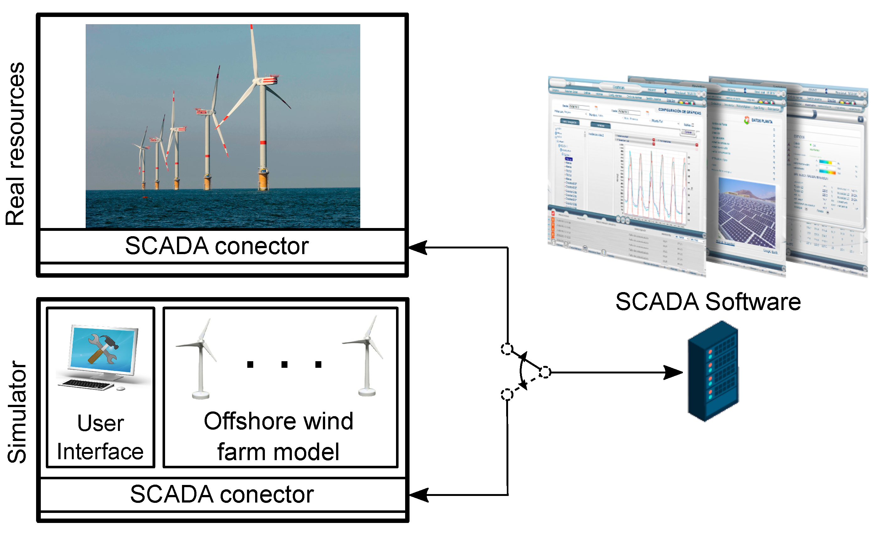
However, for a simulator like the one described above to be really useful, it should meet certain requirements. For example, it should be transparent for the user, i.e., maintaining the same interaction with both the real or the simulation plant. In this sense, as can be seen in Figure 1, users need to be able to switch between (or even combine) real and simulated DER if necessary, but always maintaining the same SCADA interface.

In a regular operation, SCADA shows the real resources’ information. However, when new operators should be trained for a specific issue, the simulation of this scenario could be executed, always maintaining the same SCADA interface.

Additionally, the simulation must also be executed in the background, evolving independently. Although SCADA could not obtain values from the simulation, the simulator would continue evolving its simulation variables. Therefore, when SCADA asks for the value of a variable, it will always get the most updated value, as when this happens in a real facility.

Finally, the simulator should be friendly for the users, providing a simple interface to configure the simulation parameters. Moreover, common SCADA users do not need to have advanced programming skills. Therefore, the simulator should provide the necessary tools to create, modify, and run DER models easily, especially designed for training purposes.

3. Simulation Tool Description

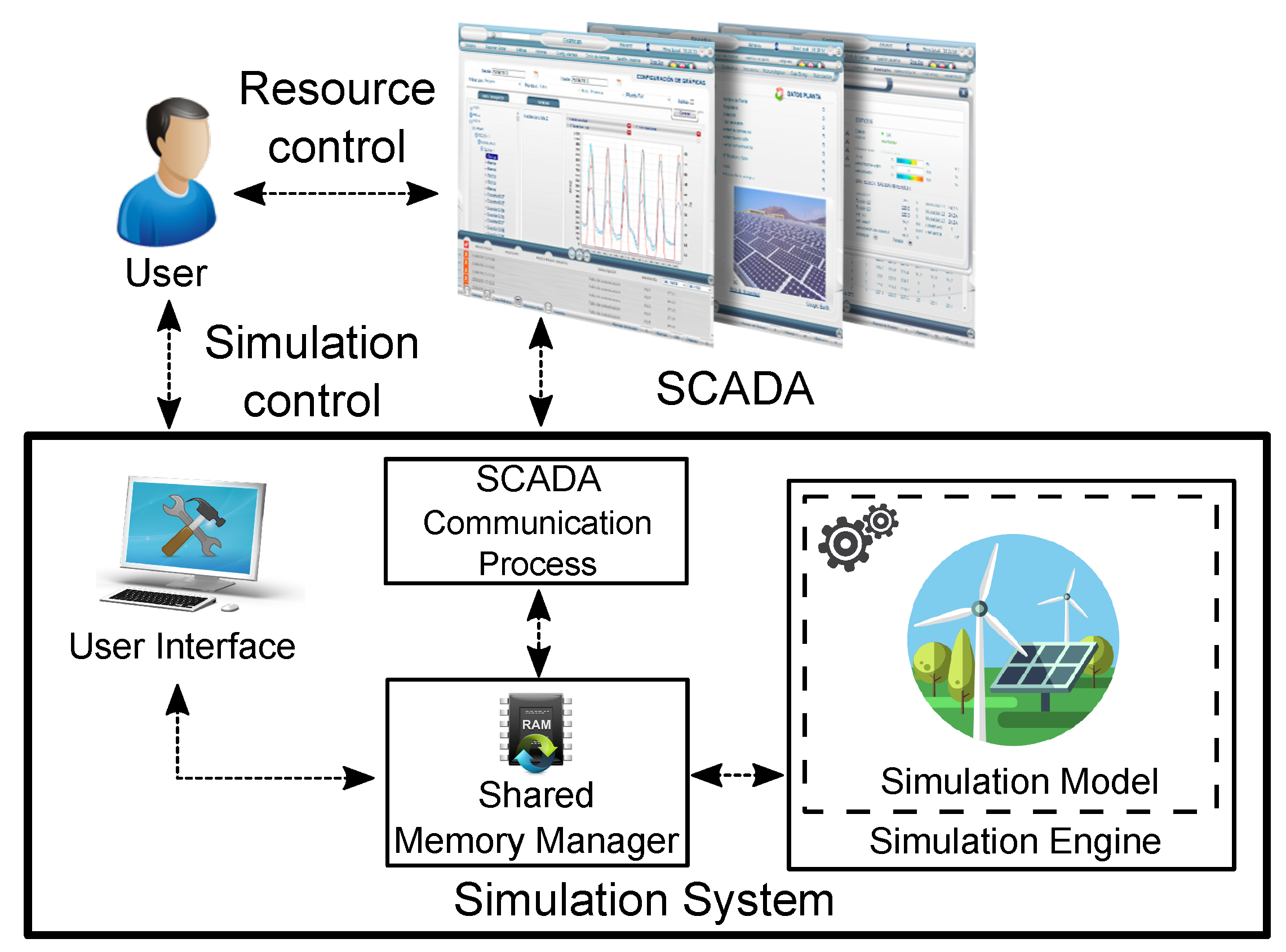
To accomplish the requisites exposed in Section 2, the proposed simulation tool was designed with the architecture depicted in Figure 2. As can be seen in this figure, the simulator was based on three different blocks that exchanged information among them. Specifically, it mainly consisted of a data repository (the shared memory manager) to manage the memory exchange between the other three blocks; the SCADA communication processand the simulation engine. Each one of those blocks is described in detail the next subsections.

The proposed simulation system was programmed as a standalone C++ application. Therefore, the shared memory manager, the SCADA Communication Process, and the simulation engine were programmed as external libraries that would be called by the simulation system’s main process itself. In this sense, all of these blocks were written as a standardized C library interface that made it possible to change or modify each one independently. Specifically, the proposed architecture allowed advanced users to change the communication method with SCADA (through the SCADA communication process) or even to change the script language for the simulation engine, but maintaining the same simulation system.

Thus, thanks to this architecture, the user could interact with the system in two ways: through the SCADA or using the configuration interface. Besides, this architecture also made it possible to combine two control scenarios for the SCADA simultaneously: with simulated and real facilities, but allowing the user to adapt the simulation model for each specific use case. The different blocks that made up the architecture of the proposed solution are described in the next sections.

3.1. Shared Memory Manager

As can be seen in Figure 2, the simulation engine, the SCADA communication process, and the configuration interface share data by means of a shared memory area. Specifically, these three processes need to be read or written in the common memory zone.

The shared memory manager controls the common memory block. This manager is responsible for maintaining the consistency of the data, even when having multiple accesses over the same data points from different processes at the same time. Specifically, this block is responsible for:

• Creating the configuration and simulation shared variables when a new simulation starts.
• Saving or providing configuration parameter values to/from the configuration interface and the simulation engine.
• Saving or providing simulation signal values to/from the SCADA communication process, the configuration interface, and the simulation engine.

In order to do that, the shared memory manager has a memory synchronization mechanism, so it ensures that the data points are consistent for the simulated models and for SCADA. This manager guarantees that one process does not change the data points of other processes in the middle of an execution step. This manager work as follows:

• If a simulator model modifies the value of a data point, this new value is immediately available for this model, but it is not immediately written into the common memory block. Thus, for SCADA and the rest of the modules, the data value has not been modified yet.
• If the configuration interface or the SCADA communication process requests a write operation, this new value is stored in a temporary location, but not in the common memory block, until all the modules are synchronized at the end of the current simulation step. For example, if SCADA sends a run operation to a DER, no block will see this order, until the next simulation step is complete. This procedure guarantees data consistency, avoiding errors coming from a data change at the middle of an execution step.
• When an execution step is finished, the new data values are synchronized in the common memory block. In the same way, before executing a new simulation step, the simulation engine copies the data values into a temporary location in order to hold the new data values coming from SCADA and the configuration interface.
• If a data point is written more than once from SCADA and/or from the configuration interface, the shared memory manager will only consider the last one, discarding the previous values.

Every data point has an identification name (ID), so it allows other processes to retrieve the data values from the common memory area. Thus, this ID must be unique.

This memory model is especially suitable for the development of Finite State Machine (FSM) models. This procedure and memory model allow the simulator to follow a strategy typically used in automation equipment, such as the Programmable Logic Controllers (PLCs), which have proven its robustness over the years.

3.2. SCADA Communication Process

This block is designed as a data gateway between SCADA and the simulation tool. In this way, there exist many alternatives of communication interfaces for SCADAs. In renewable applications, some typical standards are Modbus [39], Distributed Network Protocol 3 (DNP3) [40], IEC 60870-5 [41], and IEC 62541 (Object linking and embedding for Process Control-Unified Architecture, OPC-UA) [42], as stated in [43,44]. A special mention should be given to OPC-UA, an interesting secure [44] platform for Industry 4.0 [45].

In this sense, it is difficult to define a general exchange mechanism that covers all current SCADA solutions. Thus, as an example, a communication based on an OPC-UA interface was implemented for the proposed solution.

Moreover, the proposed modular architecture allows the system an easy adaptation to other technology. Therefore, only changing the SCADA communication library makes it possible to interact with other SCADAs or applications where a OPC-UA interface is not available.

As the rest of the simulation tool, this interface is designed to be simple and easy to maintain and is based on the next methods:

• Constructor: This method can be used to inform to SCADAs that they need to start to exchange information with the simulator, instead of the real system. It is called every time a new simulation starts.
• Destructor: This method is called at the end of the simulation. It can be used to reconfigure the SCADA communication to the real deployment.
• Connector to the memory manager: This method allows SCADA to add, read, or write data in the common memory area (as was described in Section 3.1).

3.3. Simulation Engine

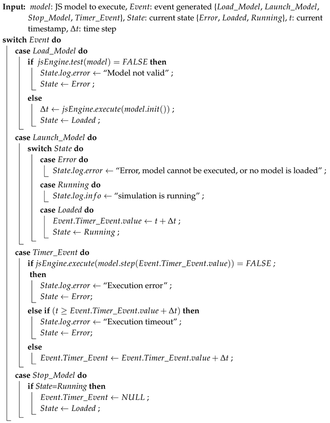
The simulation engine is responsible for executing the simulation process. This behavior is depicted in Algorithm 1, where $Event$ represents the external interaction with the applications, $State$ the internal current state of the application, and $State.log$ the standard outputs of the application.

Algorithm 1: Simulation execution cycle.

As can be seen, the simulation engine was designed as an event-based architecture. Therefore, the events could be triggered by the user or by the simulator itself. The possible events that could trigger an action were:

• Load_Model. This event is triggered when a new model is uploaded to the simulator. When receiving this signal, and after checking if the simulation model if valid, the simulator calls the init() function (see Section 3.3.2). At this point, the model is ready to be launched.
• Launch_Model. When the user wants to start or resume the simulation, this event is triggered. If the uploaded model is valid, the simulator starts a timer that will trigger a signal periodically based on the simulation step time.
• Timer_Event. During a simulation, this event is called periodically based on the simulation step time, consisting of the main simulation cycle. This event cyclically calls the function jsEngine.execute(model.step(Event.Timer_Event.value), which is responsible for the execution of the following sequence:
  • Read the inputs (signals and parameters) from the shared memory manager. If there is no new data for a required value in the simulation, it keeps the last one.
  • Run the simulation step, executing the simulation model based on the input data. This model can be made up by an aggregation of different individual submodels. Thus, in each simulation step, the following tasks will be executed:

    -

    The different individual submodels are simulated in a certain order. The order may be important, since the output of some models may be the inputs of others.

    -

    In the specific case that a final aggregation is needed, once all the submodels are simulated, the overall output data are obtained by executing the aggregation submodel. This submodel is always the last one to run in a simulation step.

  • Update the tables of input and output data on the shared memory manager with the obtained results.
• Stop_Model: When a simulation is stopped, this event needs to be called. This event stops the timer, and therefore, the simulation is stopped. In order to resume the simulation, the Launch_Model signal needs to be called again.

To do these tasks, the simulation engine was designed to execute Discrete-Event Simulation (DES) co-simulations [46], based on individual submodels defined by a Finite State Machine (FSM) [47]. The advantage of this structures is that it allows the system to know if its execution time specification is suitable for the simulation in course. Therefore, if the model execution time is greater than the defined simulation step, the simulation stops immediately, generating an error message.

Additionally, E. Byon et al. [48] implemented a DES model for a wind turbine; they stated that DES provides “hierarchical and modular model construction and an object-oriented substrate supporting repository reuse”, which is an advantage in the definition of DER models and reduces the development time.

As was described before, the simulation engine block was implemented as an external library, similarly to the SCADA communication process. Therefore, only changing the library, the proposed simulator may allow advanced users to change between different languages to define the simulation. Some examples of languages could be Network Simulator 3 (NS-3) [49], C++ [50], or Modelica [51,52,53], each one with its advantages and disadvantages. However, most of these languages have a complex learning curve and are not traditionally used by SCADA users.

In this sense, Wagner exposed in [54] that “although JavaScript cannot compete with strongly typed compiled languages (such as C++, Java and C#) on speed, it provides sufficient performance for many types of simulations and outperforms its competitors on ease of use and developer productivity”. However, according to some comparisons [55] [56], the difference in performance between a native C/C++ code and a JS implementation is in the order of 35-45%, which is similar to Java performance. Due to this and following this approach, ECMAScript 2009 [57] was chosen as an appropriate solution for the scripting language for the model simulation engine.

ECMAScript is a standardized and platform independent version of JavaScript (JS). Nevertheless, as was described in [58], modern JS engines are very efficient. Many of the performance issues are due to inefficient usage of the provided Application Programming Interfaces (APIs). In this sense, to solve this problem, a reduced extra instruction set over JS (see

Table 1. List of the extra instruction set defined for the simulation scripts.

Name	Description	Function Syntax
include	Add an external script file to the current simulation.	include(<file>);
fsRead	Read a file, and return its content as a JavaScript string.	<text>=fsRead(<file>);
fsWrite	Write the content of a JavaScript text in a file. By default, any existing file is overwritten. Alternatively, it is possible to append the content at the end of an existing file by adding an active flag (with a “true” value) as the third parameter in the call.	fsWrite(<file>,<text>); or fsWrite(<file>,<text>,<flag>);
logInfo	Send an information message to the general log. This message does not stop the script execution.	logInfo(<message>);
logWarning	Send an alarm message to the general log. This message does not stop the script execution.	logWarning(<message>);
logError	Send an error message to the general log. This message stops the simulation immediately.	logError(<message>);
addInt	Create an integer-type variable in the shared memory.	addInt(<name>,<intValue>);
addReal	Create a real-type variable in the shared memory.	addReal(<name>,<realValue>);
addText	Create a text-type variable in the shared memory.	addText(<name>,<textValue>);
getInt	Read the value of an integer-type variable from the shared memory.	<intValue>=getInt(<name>);
getReal	Read the value of a real-type variable from the shared memory.	<realValue>=getReal(<name>);
getText	Read the value of a text-type variable from the shared memory.	<textValue>=getText(<name>);
setInt	Update the value of an integer-type variable in the shared memory.	setInt(<name>,<intValue>);
setReal	Update the value of a real-type variable in the shared memory.	setReal(<name>,<realValue>);
setText	Update the value of a text-type variable in the shared memory.	setText(<name>,<textValue>);

) was provided for the proposed simulation tool.

This instruction set makes up a simple API, specifically designed for simulation purposes, reducing the complexity in the definition of simulation models. This approach improves the usability of the proposed simulation tool, making the simulation models easily modifiable by SCADA administrators, not requiring other more complex JS environments such as nodeJS [50,59,60].

However, JS still has some efficiency weaknesses. For example, it is not possible to simulate complex transients with the simulator, but its performance is enough to execute common models of DER systems, where the execution time is typically in an order of magnitude of seconds. This is especially true for training purposes, where the accuracy of the model in power generation is not the most important task.

Moreover, as was explained before, in the case of need, the JS module could be substituted by another one, based on any other more efficient language, only changing the corresponding shared library of the simulator, but maintaining its interface. Because, as described before, the simulator was designed in a modular way, each block could be substituted.

3.3.1. Simulation Model Definition

The simulation engine was designed to implement FSM. Specifically, every model should have the architecture depicted in Figure 3. As can be seen in this figure, every model should have two types of inputs (signals and parameters). Moreover, the model results are stored as outputs at the simulation end. Summing up, the description of the input/output data is the following.

• Signal inputs: This data represent the information related to the model operation. They come from SCADA or from the other submodels.
• Parameter inputs: These data represent the characteristics that define the behavior of the models (e.g., settings, threshold, limits, etc.) and the simulation scenario. They come from the configuration interface.
• Model outputs: These data represent the information obtained as a result of the execution of the different elements of the model. They will be sent to the shared memory manager (after every simulation step is finished), where they could be used by SCADA or by other models.

This notwithstanding, it is only a functional separation; all of the signals or parameters are actually stored in the same common memory area and are handled by the shared memory manager.

Taking this philosophy into account, one model could behave differently depending on its input signals and its configuration parameters. For example, it can be stopped, running or generating energy with a certain curve of generation depending on the inputs, with an anomalous behavior in which the generated energy is unusual, in a fail state, etc. In this sense, the same model can be used multiple times, with different behaviors, by calling different instances, but with different inputs.

In the proposed simulation engine, every model must implement two different parts: an initialization and the behavior for the simulation step. The initialization is responsible for creating the model interface and defining its initial behavior according to some received static parameters, as for example performance, generation curve, initial state, etc. Later, a behavior could be defined as an FSM for its execution in each simulation step. This part of the model will be responsible for obtaining the outputs according to the combination of the inputs and the current state of the model.

3.3.2. Description Model Language

As previously mentioned, the models are defined by means of scripts written in JS. In order to be executed in the simulation engine, two main functions have to be defined: the init() function and the step() function. The structure of the scrips of the models are depicted in Algorithm 2.

Algorithm 2: Structure of a model.

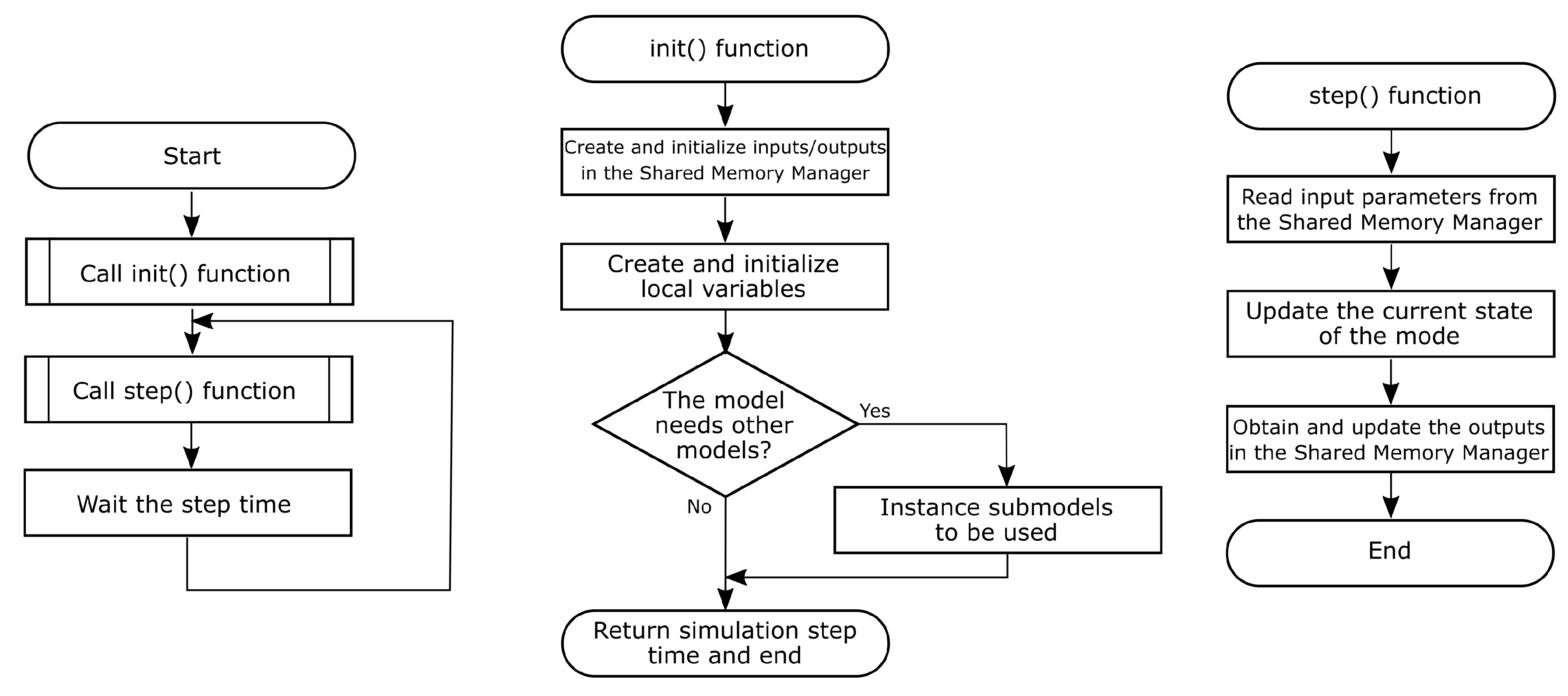
Firstly, the init() function is responsible for initializing the model. It is executed using the jsEngineAPI, designed to call JS codes from a C++ Application. In init(), the signals shared with SCADA or other submodels (through the shared memory manager) and the local variables used by the model must be created and initialized. Additionally, this function must return the required simulation time step to the simulation engine. If the model needs to use other submodels, they should be initialized in this function.

Once the simulation starts, the step() function is called periodically with the simulation time step returned by the init() function. The step() function is responsible for executing all the actions associated with each simulation step: read the inputs, obtain the next state of the simulation model, and obtain the outputs. Additionally, this function receives a parameter that allows the model to know how long the model has been active since it was started; this is especially useful for, at some point, simulating specific scenarios (errors, overgeneration, etc.) with which the operators could train.

As a summary, when a simulation is running, the system is executing the flow depicted in Figure 4.

3.4. User Configuration Interface

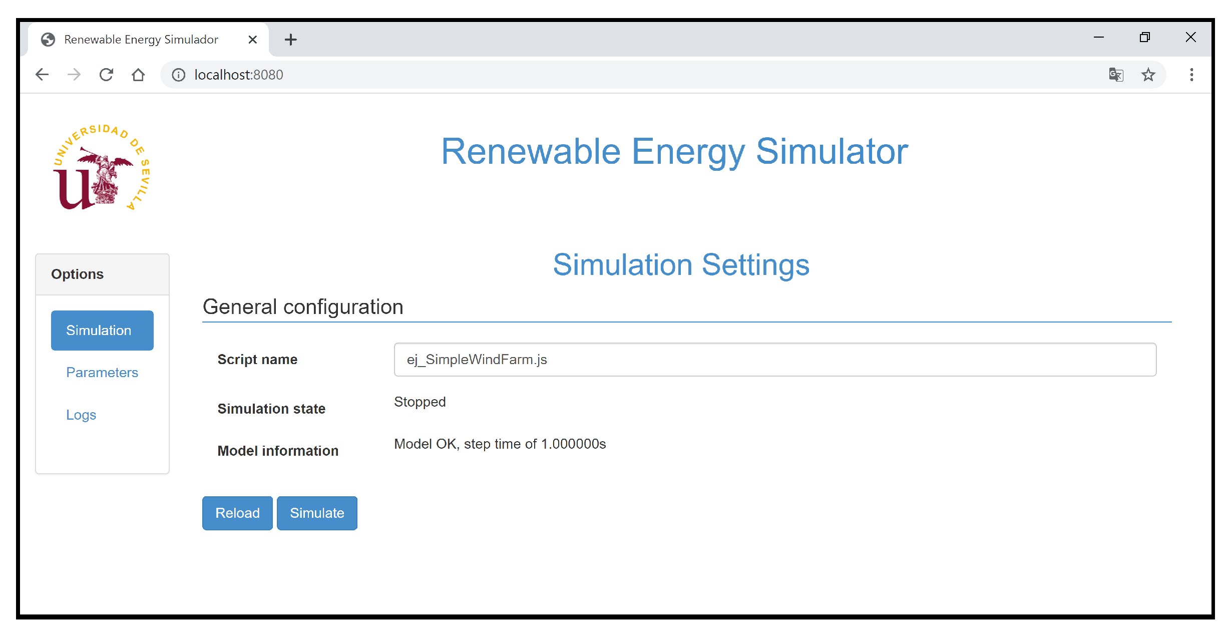
The simulator includes a configuration interfacein order to set the model parameters and to manage the simulation engine. This interface is a web-based application that can be used with a standard web navigator. This web interface has three main interfaces: simulation, parameters, and logs(see Figure 5). All the described functions can be managed from these three interfaces.

• Simulation interface: Using the Simulation interface, the user can load different scripts of DER models in the simulator. When a new script is loaded into the simulator, it checks that the script is correct and able to be executed in the simulation engine. At this moment, the user can run the script. Scripts can also be stopped and restarted using this interface.
• Parameters interface: This interface shows the available inputs and their values in the common memory area. These values can be monitored and modified using this interface, even if the simulation engine is running. For example, this interface could be used to define the initial values of a model, before it is running. Data values can be written in single mode or in group mode, where all parameters of the group will be modified simultaneously.
• Logs interface: This interface contains logs of the current simulation. These logs come from the different modules of the simulator and from the different model scripts under simulation, using the extra instruction set designed for this purpose (see Table 1). Therefore, this interface is useful for the monitoring of the whole system and its evolution. This interface is also important for debugging purposes. For example, if a model has a syntax error, it is summarized in the log, next to its line number. Moreover, if the model has an execution error (as if it cannot guarantee the time step), this information is also added.

4. Simulation Tool Abilities

As was described in previous sections, the main application of the proposed simulation tool is to train operators of renewable DER systems. Due to this, and as will be seen in the case of a real application (Section 5), the proposed JS simulation models are simple to understand, allowing the users to develop and tune their own models. However, beyond the application of this tool in training stages, its functionality can be extended to cover a wide set of scenarios.

In this sense, with the intention of showing the versatility of the proposed tool and where it can be used, this section briefly describes some applications and models that can be easily implemented over the proposed tool, mainly for training purposes, but also for other uses. Specifically, two sets can be distinguished: data sources and renewable DER models, where the first set characterizes the typical inputs of the models of the second set.

4.1. Data Sources

In renewable DER systems, a renewable energy source (i.e., solar irradiance in PVs or wind in turbine generators) is obviously necessary. Therefore, in many application, it is important to model their availability. One alternative to define these models is the use of AutoRegressive Moving Average (ARMA) time series, which is a common approach to generate synthetic information in both wind speed [61] or solar irradiance [62] scenarios. ARMA(p,q) refers to a model that adds p autoregressive terms with q moving-average terms, according to the expression of Equation (1).

$$X_t=\sum _{i=1}^p{\varphi }_i{X}_{t-i}+\sum _{j=1}^q{\theta }_j{ϵ}_{t-j}+{ϵ}_t$$

(1)

where $X_t$ is the actual wind speed at a certain time, ${\varphi }_i$ are the p autoregressive coefficients, ${\theta }_j$ are the q moving average coefficients, and ${ϵ}_t$ is a white noise that can be generated using a JS function as for example Math.random(). The main shortcoming of the ARMA model to generate renewable data sources is that this model considers a stationary time series. Due to this, to deal with seasonal trends, some authors proposed the use of seasonal ARMA, adding trend functions based on a probability distribution such as Weibull [63] or using the AutoRegressive Integrated Moving Average (ARIMA) [64], a more computationally intensive algorithm.

Another common method relies on the use of Artificial Neural Networks (ANNs), for both irradiance [65] and wind speed [66]. An ANN is composed of a number of highly interconnected processing elements $Y_{i,j}$, called neurons, where each output follows Equation (2):

$$Y_{i,j}=g\left(b_{i,j}+\sum _{k=1}^n{\omega }_{i,j,k}·Y_{i,j-1}\right)$$

(2)

where i and j represent the rows and columns of the network and $g\left(x\right)$ the activation function, ReLU (Equation 3) currently being the most used one [67].

$$g\left(x\right)=max(0,x)$$

(3)

This method can offer a very good accuracy, but it has an elevated computational cost, especially for large networks as current deep learning models propose (e.g., [68]). Therefore, this approach could not be adequate for applications with fast simulation with a reduced time step. Nevertheless, it can be implemented in JS, using libraries such as Machine Learning in the Browser (MLitB) [69], which even supports, in some cases, GPU acceleration.

However, all those methods lack an important thing. They are focused on generating information in normal operational conditions, but not under anomalies. For example, in training applications, the proposed tool could be used to repeat specific patterns that represent anomalies (i.e., high temperature, wind issues, untwisting, etc.), which could be directly obtained from historical incidences of a real installation or manually generated to force specific conditions.

In this sense, the provided tool allows reading these values from external files, for example the Comma Separated Value (CSV) format. Moreover, it is important to consider that using external CSV does not reduce the capacities of the solution, due to it not being incompatible with the use of synthetic data, which can be obtained, for example, from tools such as ClimGen [70].

4.2. DER Models

Once the external data (not defined by the user) are available, the next step is to apply them to the DER production models. Thus, these inputs are not the only ones in the submodel. Additionally, the user control signals should also be considered. Thanks to this architecture, depending on the model chosen, the operators could obtain different behaviors for the same simulation scenarios based on their actions. In this sense, to understand the proposed simulator’s abilities, this subsection identifies some models that could be easily implemented with the proposed tool and that might be able to simulate different configurations of these resources. Specifically, this study was carried out for the two main sources of renewable energy that are currently growing: solar systems and wind power systems. Thus, as will be seen below, these models may not have a complex implementation, so they can be easily applied in the proposed simulation tool.

4.2.1. Wind Power Systems

Roughly, a wind farm could be seen as an aggregation of a set of individual wind turbines. Therefore, the overall system could be characterized by the different functions of each one separately. Traditionally, this behavior is characterized by the power curve, a relationship between the wind speed and the active power generation. In this sense, manufacturers usually provide this curve in their technical data. However, this is usually generic for the turbine model and does not fully conform to reality. Due to this, statistical methods to fit this curve are a common solution [71,72]. Some authors proposed models based on polynomial regression [73]. Specifically, approaches with local approximations for the power curve, like the B-spline curves, have shown good results [74]. However, recent studies like [75] proposed monotone smooth regression to improve this approximation.

In this sense, it is important to note that this improvement model only complicates the characterization process, establishing specific continuity restrictions. Besides, its execution does not change; it is based on a third degree polynomial function (see Equation (4)), defined for each interval as:

$$aP\left(w\left(t\right)\right)=\left[\begin{array}{cccc}{p}_{i,1}& p_{i,2}& p_{i,3}& p_{i,4}\end{array}\right]\left[\begin{array}{c}w{\left(t\right)}^3\\ w{\left(t\right)}^2\\ w\left(t\right)\\ 1\end{array}\right]if\left\{\begin{array}{c}i\in \mathbb{N}=\left[1,n\right]\\ i:W{S}_{min\_i}\le w\left(t\right)<W{S}_{max\_i}\end{array}\right.$$

(4)

where n is the number of uniform intervals (defined by knots) in which the spline has been divided, each of them being bounded between a minimum ($W_{min\_i})$ and maximum $W{S}_{max\_i}$ wind speed value. Thus, $\left[p_{i,1}{p}_{i,2}{p}_{i,3}{p}_{i,4}\right]$ is a vector with the coefficients a, b, c, and d of the polynomial, obtained as the row i from the weight matrix p.

Further, other more complex methods as Hidden Markov Models (HHMs), ANNs, or Support Vector Machines (SVMs) have also been proposed. In this sense, the work in [76] made an extensive study in this way. However, these approaches demand a higher computational cost. Therefore, in this work, the approach outlined above will be appropriate in most cases.

4.2.2. PV systems

Like wind generation, solar energy is another renewable energy that is increasing its share in the last few years. In this sense, the work in [76] showed an interesting review of methods (based on Random Forest (RF), k-Nearest Neighbors (k-NN), etc.) to estimate the solar production. However, these approaches only model the system. They do not allow the necessary flexibility to be used for a simulation in tools like the proposal.

As an alternative, solar farms could also be seen as some aggregation of photovoltaic subsystems (PV panel + inverter), whose generation is directly related to the solar irradiation that they receive. In this sense, Kazem and Khatib [77] showed a parametrical model of this set. PV panel generation is characterized by Equation (5). Specifically, its output power increases linearly with the solar radiation $G\left(t\right)$, but decreases with the ambient temperature $T_{amb}\left(t\right)$.

$$P_{PVpanel}\left[G\left(t\right),T_{amb}\left(t\right)\right]=P_{Peak}\left({\displaystyle \frac{G\left(t\right)}{G_{std}}}\right)-\left\{{\alpha }_T\left[{\displaystyle \frac{NOCT}{800}}G\left(t\right)+T_{amb}\left(t\right)-T_{std}\right]\right\}$$

(5)

where $G_{std}$ and $T_{std}$ are the standard PV test conditions, ${\alpha }_T$ is the temperature coefficient, and $P_{Peak}$ is the panel rated power. Thus, $NOCT$ is the nominal operating cell temperature (experimental data of the panel measured for 800 W/m${}^2$, at $T_{amb}=20{}^{\circ }$C, and under a wind speed of 1.5 m/s). These data were defined in the manufacturer’s datasheet.

Thus, similarly to the PV panel, the inverter could be also characterized, in this case with the addition of a performance parameter ${\eta }_{INV}$, defined by Equation (6):

$${\eta }_{INV}={\displaystyle \frac{P_{in}-P_{loss}}{P_{in}}}$$

(6)

${\eta }_{INV}$ makes it possible to estimate the total generation of the systems $P_{PV}$, following Equation (7):

$$P_{PV}={\eta }_{INV}·P_{PVpanel}\left[G\left(t\right),T_{amb}\left(t\right)\right]$$

(7)

where $P_{in}$ is the input power and $P_{loss}$ represents the energy lost in the conversion process. Thus, the performance of an inverter is supplied by the manufacturer (typically around $95\%$), but it usually has lower values if it is below $30\%$ of its capacity.

4.2.3. Energy Storage Systems

Other crucial elements within DR systems are the Energy Storage Systems (ESS). Thus, the detailed modeling of these elements can be complex. However, for an electrical system, they can be seen as point energy stores, whose availability is usually represented through the State-of-Charge (SoC) of Equation (8), where $SoC\left(t\right)$ is the SoC (in p.u.) of the system in each moment, $SoC(t-1)$ is the SoC at the previous simulation step, $P_{out}$ is the power delivered by the ESS along the period $\Delta t$, and $C_{ESS}$ is the energy capacity (in KWh).

$$SoC\left(t\right)=SoC(t-1)-{\displaystyle \frac{P_{out}}{C_{ESS}}}·\Delta t$$

(8)

Thanks to the simulator architecture and its ability to associate memory with each model, it is possible to implement this kind of resource in an easy way.

5. Study Case

One proof of the usefulness of the proposed tool could be found in the application where it was developed. This simulation tool was developed as a part of the SEAPEMproject, which is focused on developing a system for offshore wind farm support. Specifically, the proposed simulation tool was developed for its integration with the Bluence^® suite by Isotrol^® [78], A a complete Information and Communications Technology (ICT) solution that makes it possible to manage large amounts of data in renewable energy plants. Bluence^® is the core of the Bluence^® Control Center (see Figure 6), a 24/7 support center for renewable energy power plants.

Bluence^® Control Center has been designed to support tasks such as redundancy and security, the dispatching center, incident management, and 24/7 remote support. It is in this scenario where Isotrol^® detects the lack of simulation tools specifically designed for operator training, or for the start up of new SCADAs, scenarios where the proposed simulator becomes an interesting utility for planning, operation, and testing tasks.

Moreover, to understand the usefulness of the proposed simulation tool really, it is interesting to analyze some practical application examples. Therefore, this section describes in detail three functional models that make it possible to understand its potential integration for SCADAs with renewable energy management in training operator tasks. In this sense, one of the most relevant technologies of this kind of energy source is wind generation. Due to this, the proposed examples focus on this technology. However, it is interesting to highlight the possibilities of the simulator, allowing different levels of model accuracy. Besides, as described before, it can model plants of other technologies such as: PV, Combined Heat and Power (CHP) plants, etc.

Specifically, three models are described in next subsections. The first one describes a wind farm of ten generators using a simple turbine model. Later, the second applies an empirical model of a wind turbine, using monotonic splines. Finally, the last one proposes a more complex turbine model focused on training SCADA users over different scenarios.

5.1. Wind Farm with a Turbine, Simple Model, Based on the Manufacturer’s Specifications

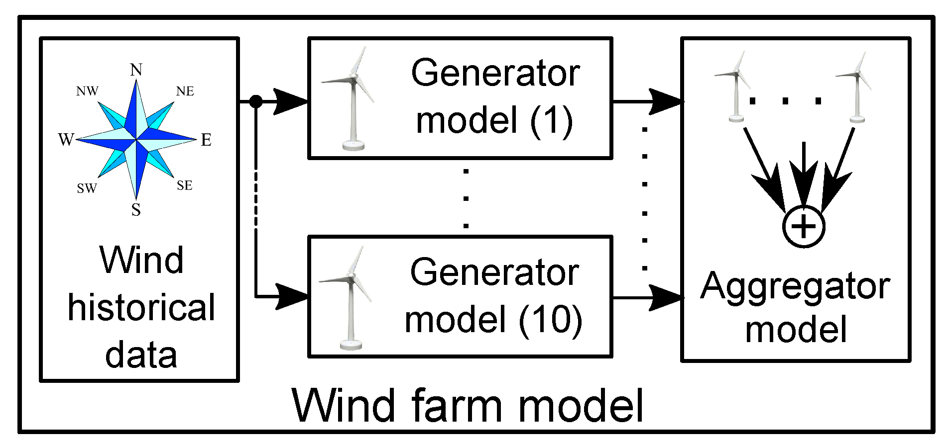
The capability of simulating the behavior of an asset is very interesting for facilities setting up and training their users. Obviously, the model actually depends on the specific use and the required precision. In this sense, the first example proposes an implementation of a simple wind farm model. This model proposes a hierarchical implementation (as can be seen in Figure 7), following the model philosophy described in previous sections, and using three submodels: one for the load wind historical dataset (see the code in Appendix A.1), another to implement a simple turbine model, which is directly based on the manufacturer’s power curve (see the code in Appendix A.3), and the last submodel to aggregate the overall generation of the wind turbine set (see the code in Appendix A.2).

// ej_Simple_Wind_farm.js: Simulation example for aggragation of 10 simple wind turbines. include(’LibSubmodels/Submodel_SourceFile.js’); include(’LibSubmodels/Submodel_WindTurbine.js’); include(’LibSubmodels/Submodel_Aggregator.js’); // Simulation parameters. var aggregatorId = 0; var startSrcId = 11; var windSrcId = 12; var turbineId = [1,2,3,4,5,6,7,8,9,10]; var model = “ECOTECNIA 74/1670”; var stopTime = 60; var windTable = [0,2,3,4,5,6,7,8,9,10,11,12,13,25]; var powerTable = [0,0,7,50,118,226,378,580,840,1138,1463,1640,1670,1670]; var initDate = “01-nov-2017”; var initTime = “12:00:00.0000”; var windFile = “Signals/wind_”+initDate+“.csv”; var startFile = “Signals/start_”+initDate+“.csv”; // Sumodel instances. var startSrc = new Submodel_SourceFile(startSrcId,“Start Source File”); var windSrc = new Submodel_SourceFile(windSrcId,“Wind Source File”); var turbines = new Array(turbineId.length); for (i=0 ; i<turbineId.length ; i++)  turbines[i] = new Submodel_WindTurbine(turbineId[i],model,windTable,powerTable,stopTime); var aggregator = new Submodel_Aggregator(aggregatorId); // Init function definition. function init() { var timeStep = 1;  startSrc.init(timeStep,initDate+“ ”+initTime,startFile);  windSrc.init(timeStep,initDate+“ ”+initTime,windFile);  for (i=0 ; i<turbineId.length ; i++)   turbines[i].init(timeStep);  aggregator.init(timeStep,turbineId,“activePower”,“totalPower”);  return timeStep; }; // Step function definition. function step(timeStamp) {  startSrc.step(timeStamp); windSrc.step(timeStamp);  for (i=0 ; i<turbineId.length ; i++)   turbines[i].step(timeStamp,getReal(“srcValue”+startSrcId),getReal(“srcValue”+windSrcId));  aggregator.step(timeStamp);  return 1; };

As can be seen in the code of the proposed model for training SCADA users, this implementation loads the different submodel files from a repository, creates the common signals between them, and defines the required main init() and step() functions. In this case, these two main functions are made up as a sequence of calls of the init() and step() functions of each submodule.

Specifically, as can be seen in the previous script, the implementation of the wind farm model was made up by ten turbines, fed with the same wind source. These operations were characterized by their power curve (the relation between the wind speed and the generated power) of the turbines, Model 74/1670 by the ECOTECNIA manufacturer for this case (see

Table 2. ECOTECNIA 74/1670 behavior *.

Wind Speed (m/s)	Power (kW)	Power Coefficient CP (-)	Thrust Coefficient CT (-)	Wind Speed (m/s)	Power (kW)	Power Coefficient CP (-)	Thrust Coefficient CT (-)
1	0	-	-	14	1670	0.23	0.30
2	0	-	-	15	1670	0.19	0.24
3	7	0.10	1.04	16	1670	0.15	0.20
4	50	0.30	0.88	17	1670	0.13	0.16
5	118	0.36	0.77	18	1670	0.11	0.14
6	226	0.40	0.78	19	1670	0.09	0.12
7	378	0.42	0.79	20	1670	0.08	0.10
8	580	0.43	0.79	21	1670	0.07	0.09
9	840	0.44	0.79	22	1670	0.06	0.08
10	1138	0.43	0.73	23	1670	0.05	0.07
11	1463	0.42	0.67	24	1670	0.05	0.06
12	1640	0.36	0.53	25	1670	0.04	0.05
13	1670	0.29	0.39

* Note: Measurement conditions: Density = 1.225 kg/m${}^3$, height = 0 m, and temperature = 15 ${}^{\circ }$C.

). To do that, after the init() function’s definition, this model instantiates a simple wind turbine submodel ten times (see the code in Appendix A.3), setting the specific configuration in the definition of each one.

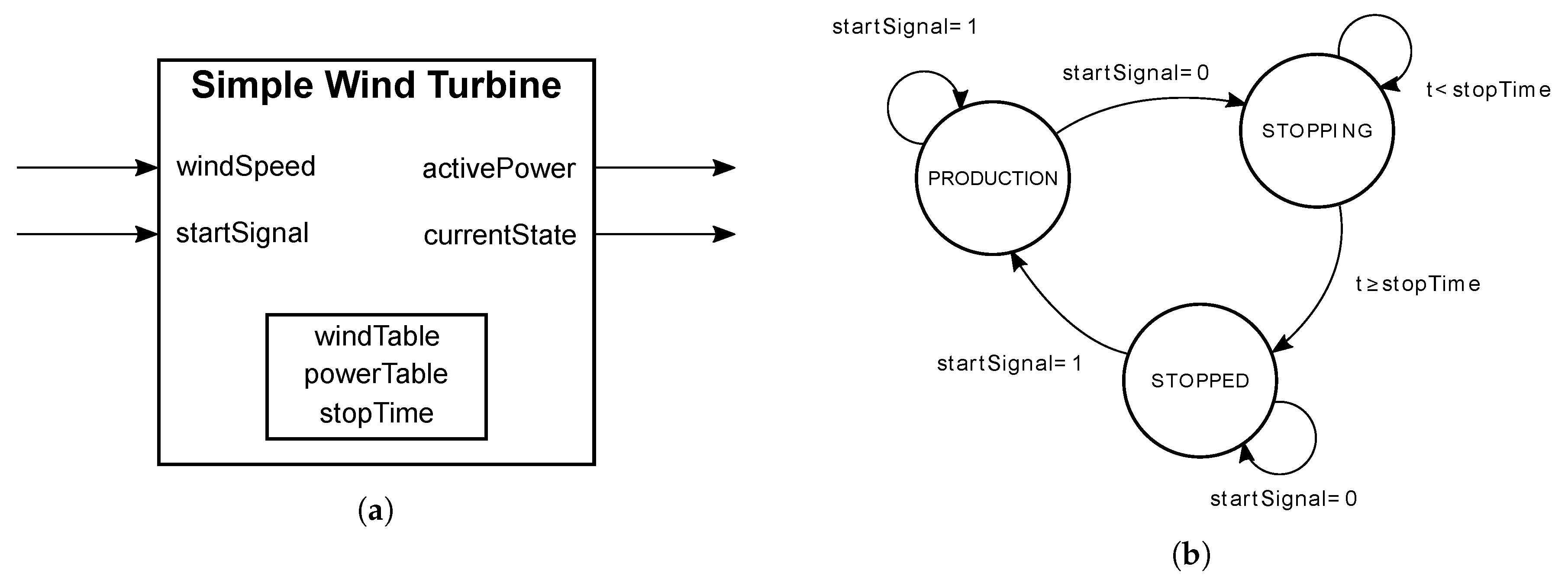
This turbine submodel characterizes an FSM whose interface and behavior (state diagram) are shown in Figure 8. Specifically, this submodel has three states: the PRODUCTION state, which represents when the turbine is in normal generation mode and following the power generation curve, the STOPPED state, which represents when the turbine is completely stopped, and the STOPPING state, which characterizes the stopping behavior when an stop order is received.

In standard operation, the active power, $aP\left(w\left(t\right)\right)$, generated by the turbine will be obtained by a piecewise linear interpolation, through Equation (9), where parameter $w\left(t\right)$ represents actual wind speed input and WS and P are respectively the wind speed and active power reference data, obtained form Table 2, both in the ${\mathbb{R}}^{1xn}$ range.

$$aP\left(w\left(t\right)\right)=\left\{\begin{array}{ccc}P\left[1\right]& if& w\left(t\right)<WS\left[1\right]\\ {\displaystyle \frac{P[i+1]-P\left[i\right]}{WS[i+1]-WS\left[i\right]}}·\left(w\left(t\right)-WS\left[i\right]\right)+P\left[i\right]& if& \left\{\begin{array}{c}i\in \left[1,n-1\right]\\ i:WS\left[i\right]\le w\left(t\right)\le WS[i+1]\end{array}\right.\\ P\left[n\right]& if& w\left(t\right)>WS\left[n\right]\end{array}\right.$$

(9)

Thus, the model output activePower is calculated depending on the current state, as can be seen in

Table 3. Wind turbine activePower generation depending on the current state.

STATE	PRODUCTION	STOPPING	STOPPED
activePower	$aP\left[w\left(t\right)\right]$	$\left(1-{\displaystyle \frac{t-t_0}{stopTime}}\right)·aP\left[w\left(t\right)\right]$	0

, and taking into account that t is the current time, $t_0$ is the instant when starting the stopping action, and stopTime the time to stop.

As Section 4.1 describes, we propose to obtain the wind profile from from external files in CSV format. As described before, training users on security assets requires generating specific patterns during the training, as happens in abnormal scenarios, such as high winds or gusts. Common models to forecast or generate synthetic winds usually do not allow this, it being easy to obtain this information from incidences of the historical database of the real system.

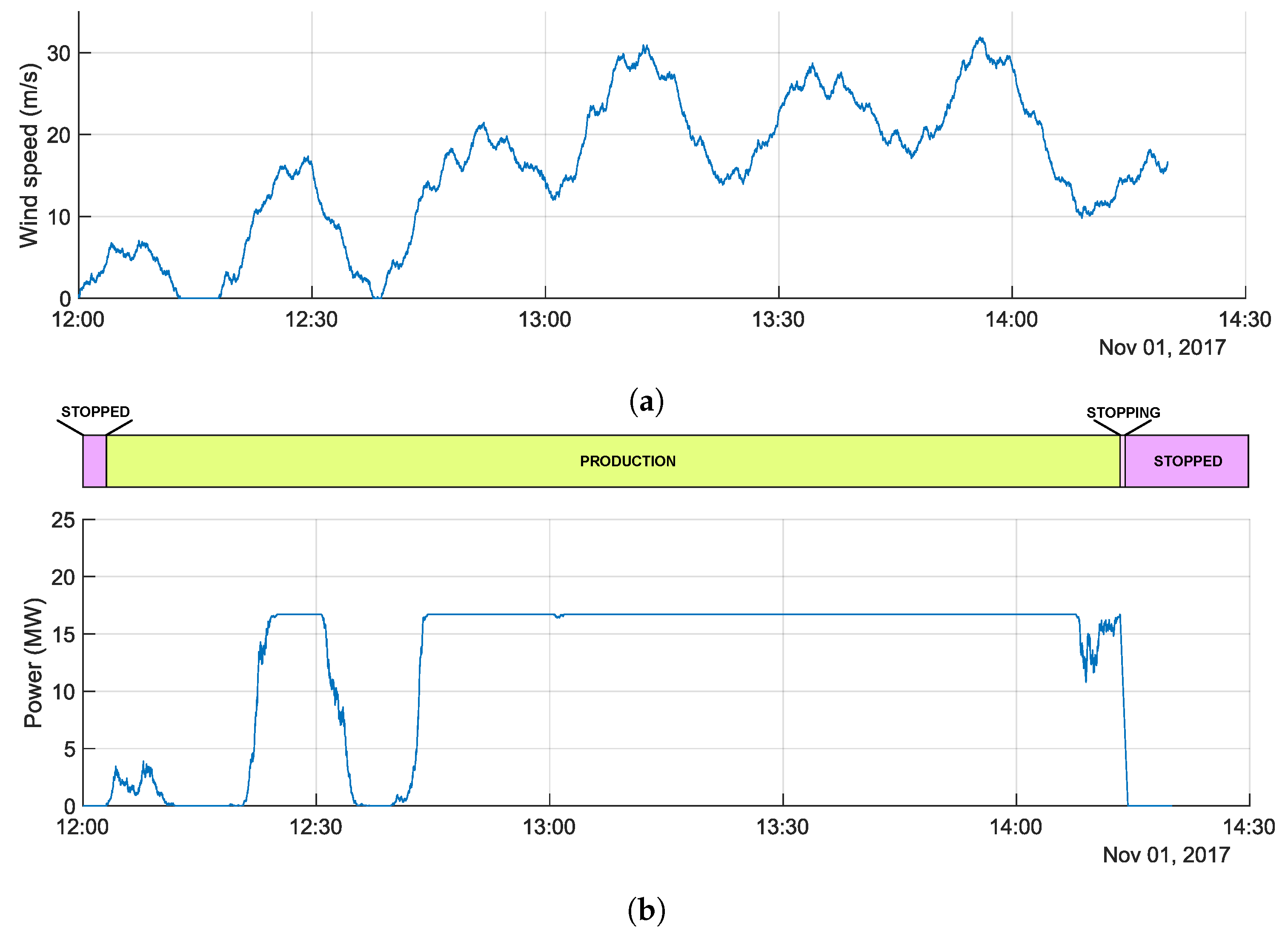
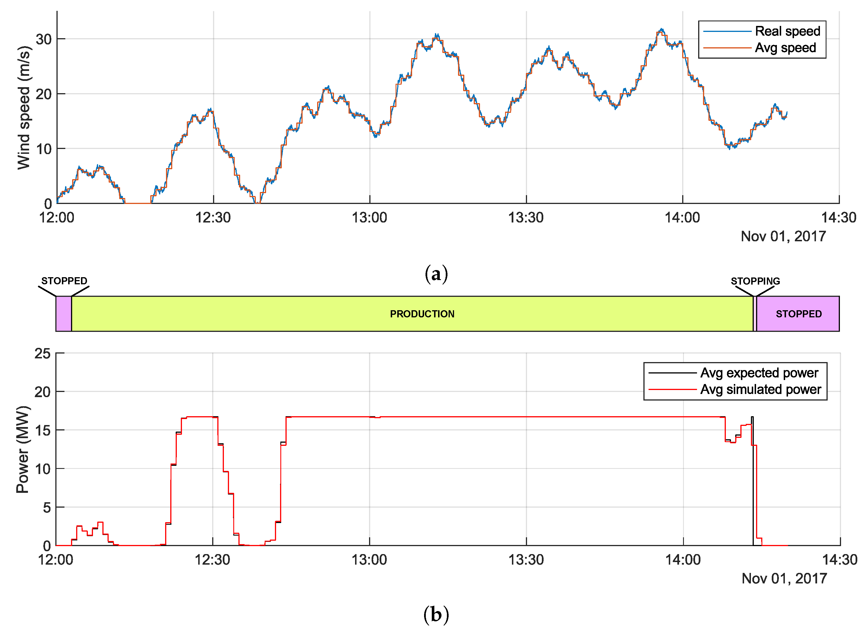
Using the proposed model for this study case and exciting it with a wind profile based on historical signals, it was easy to simulate the behavior of the overall wind farm with different time steps (as can be seen in Figure 9, Figure 10 and Figure 11).

In these figures, three cases were simulated for the previous wind farm with the same wind profile for two hours and twenty minutes. In this case, in order to simplify the model, all wind generators were fed with the same wind profile, but different ones could be used as input for each one if desired. Figure 9 is the most accurate simulation, with a simulation step of one second (1 s); Figure 10 has a step of one minute (1 min); and Figure 11 has a simulation step of ten minutes (10 min). Thus, Figure 9 was used as a reference for Figure 10 and Figure 11 to understand with an example the strong relationship that can exist between the simulated power error and the simulation time step.

Specifically, with the same wind profile, using a 1 min simulation step, the absolute error in the generated power simulation was 1.26%. However, using a 10 min simulation step, this absolute error increased up to 8.99%.

Thus, once the simulation scenario was defined and it was verified that the simulation was possible, the next step should be the comparison between the real and the simulated generated data. However, this analysis was only done in intervals of 10 min, because the available dataset from a real wind farm facility (see

Table 4. Historical dataset details.

Description	Value
Total time	9480 h (13 months)
Total time in production state	4645.3 h
Average power real (in production state)	763.45 kW
Average power expected (in production state)	617.50 kW
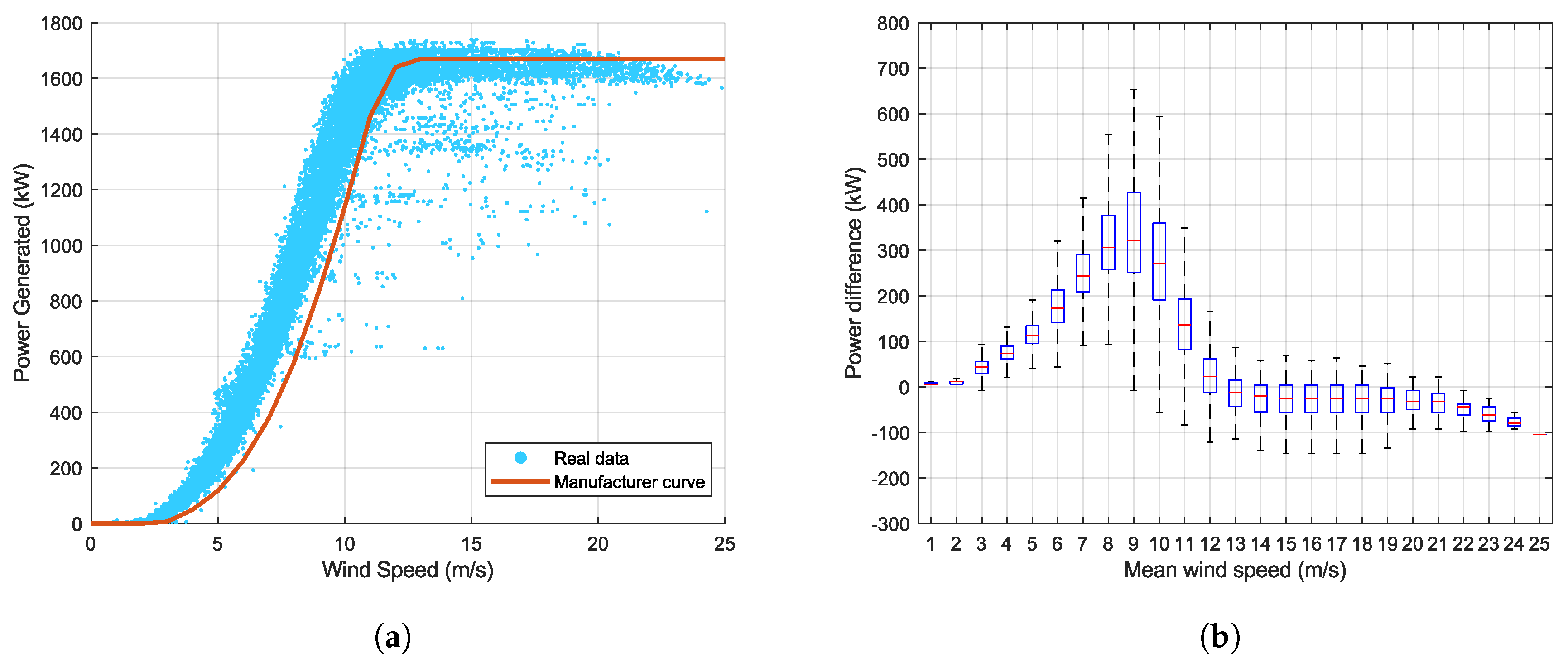
Power error	21.90%

with an example of turbine generation data details) only contained records of wind speed and generated energy at this frequency. Thus, taking into account that the power curve of wind turbines is a non-linear function (as can be seen in Figure 12b), the simulation for these average wind speed values did not completely match the real generation, but it was not a big issue in the training applications. This error strongly depended on the distribution of wind speed along time.

This fact is depicted in Figure 12 where the difference between the real and simulated generation is plotted as a function of the wind speed. The error represented was the signed difference between the real power generator during every 10 min period and the estimated power. Specifically, the estimated power was obtained assuming the average wind speed and the manufacturer curve during the same period. This figure was made up from the available dataset using only one turbine record.

A curious effect appears in Figure 12b, which represents its distribution error (error between the real data and the manufacturer’s power curve). On the one hand, from 3 m/s (the start of the production) until about 13 m/s, the distribution error was mainly positive (the turbine generated a power greater than that corresponding to the mean of the wind speed, assuming the power curve). Of course, in this interval, the second derivative of power curve was positive, and this explained why the difference was positive. On the other hand, from 13 m/s until 25 m/s, the second derivative was negative or zero. Of course, this caused the distribution error of the power difference to be negative due to the distribution of wind speeds. This was why from wind speeds of 13 m/s and higher, the experimental power values were less than the expected according to the manufacturer curve. Therefore, in this zone of the graph, the mean errors resulted in being negative.

To sum up, those differences in the real data were normal and understandable. Therefore, the simulated data recorded each ten minutes were not enough to obtain accurate results to reflect the dynamics of a wind turbine faithfully. Nevertheless, it is important to note that the goal of this paper is not to propose an accurate wind turbine model, for which, as previously shown, it would require a dataset with a higher temporal resolution. As was discussed throughout this paper, this is focused on the development of an operational simulation tool designed to be integrable in a SCADA, which allows training or testing by operators in a safe way for real facilities. In this sense, the power curve from the manufacturer was a valid approximation for a learning application. Using this simple model, an operator could observe the relation between both variables and check if the power was at the adequate limits. A power generation beyond those limits would suppose a problem in the turbine, which should be managed and solved by the operator.

With all of the above, this does not mean that the proposed tool did not allow the simulation of precise models. However, the proposed models were more focused on a correct representation of the operational evolution of the system than on a faithful representation of the behavior of the turbines. Nevertheless, if the main goal were implementing a more precise model, this improvement was compatible with the proposed tool, only writing a script that would define its behavior.

Furthermore, to show the simulation capacity of the proposed system, some performance results were obtained with a PC with an Intel^® Core^TM i5-6400T CPU with 8GB of RAM. Using the proposed simulator and the model of this subsection, which consisted of the aggregation of a series of wind generators, this model was executed using different numbers of generators, obtaining as a result a mean value of 10.93 microseconds of execution time per generator in every step.

Based on this result, it was possible to obtain the maximum number of generator instances that could be used for a fixed time step. For example, using one second as a time step in the aforementioned PC, the maximum number of generator instances was 91,743 for a valid on-line simulation. It is important to remember that, as described before, in order to be a valid simulation, the time step needed to be higher than the execution time required by the models.

5.2. Wind Farm with a Turbine Model, Obtained from Empirical Data

This example describes another application scenario. In this case, a wind turbine empirical model was based on a a monotone smooth regression spline [75], previously discussed in Section 4.2.1. This example had two objectives: (a) demonstrate how a previous model could be easily adapted or modified by an operator; (B) show how to implement in the simulator the models depicted in Section 4.

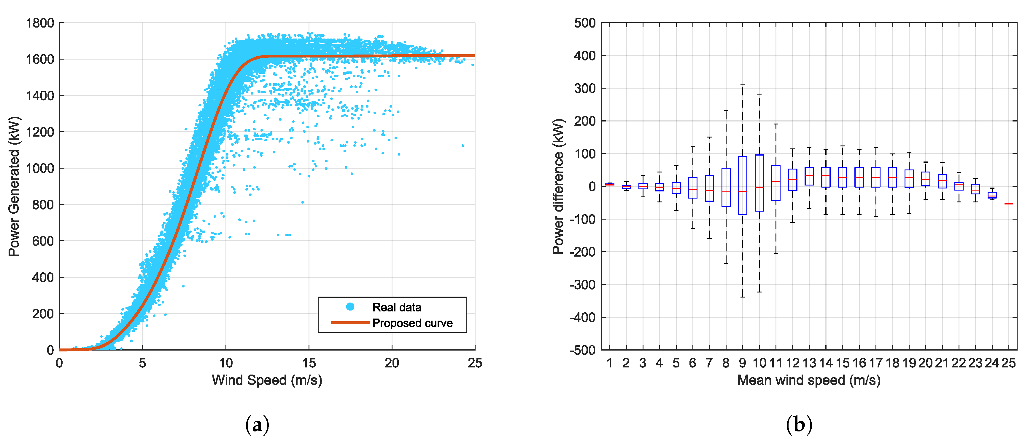
The empirical information used to model the wind turbine was obtained from a historical dataset from a wind farm based on ECOTECNIA 74/1670 wind generators, the same depicted in Table 4. Using this dataset and following Mehrjoo et al.’s procedure [75], the empirical model depicted in Figure 13a was obtained.

In this case, the monotonic spline was divided into 25 uniform intervals (defined by 26 knots), whose coefficients a, b, c, and d conformed to the matrix of coefficients p, which are used in Equation (4).

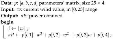
The use of 25 intervals and considering that the wind speed was limited in the operational range (speeds out of this range caused the turbine to stop), the power from wind speed and using this model could be obtained using the Algorithm 3, as can also be seen in the JS code below.

Algorithm 3: Power estimation with monotonic spline.

const p = [[-2.3382,4.0083,0,1.0287e-07],[6.851,-23.559,27.568,-9.1892],   [2.9074,0.10221,-19.755,22.359],[-3.3688,56.588,-189.21,191.82],   [3.5426,-26.348,142.53,-250.51],[-1.3627,47.23,-225.36,362.64],   [1.6336,-6.7022,98.235,-284.55],[-6.8934,172.36,-1155.2,2640.2],   [-8.3494,207.31,-1434.8,3385.7],[-11.558,293.95,-2214.6,5725],   [-0.0096583,-52.51,1250,-5823.7],[11.195,-422.28,5317.5,-20738],   [6.4142,-250.15,3252,-12476],[-4.9439e-10,1.2205e-08,-2.6495e-09,1616.3],   [2.2112e-08,-9.3881e-07,1.3333e-05,1616.3],[9.1158e-09,-3.5556e-07,4.6082e-06,1616.3],   [-4.9996e-08,2.4802e-06,-4.0739e-05,1616.3],[0.31814,-16.225,275.83,53.303],   [-0.7423,41.038,-754.92,6237.8],[0.84817,-49.618,967.56,-4671.2],   [-0.74202,45.793,-940.67,8050.2],[0.318,-20.988,461.74,-1766.6],   [-1.2137e-06,8.2095e-05,-0.0018491,1619.5],[1.7214e-06,-0.00012043,0.0028089,1619.5], [-3.3594e-06,0.00024539,-0.0059707,1619.6]]; function aP(w) { var i;  if (w < 0) i = 0;  else if (w > p.length) i = p.length-1;  else i = Math.floor(w);  return p[i][0]*w^3 + p[i][1]*w^2 + p[i][2]*w + p[i][3]; };

As can be seen in Figure 13, this model offered better accuracy than the previous one. However, it is important to remark that accuracy in power estimation is not the main goal of a tool designed for training SCADA users. Simplicity to adapt to new scenarios and to have a correct behavior that can be simulated in real time are more important factors. However, this class of models demonstrated the abilities of the simulator to be used in different applications.

5.3. Wind Turbine Complex Model

In order to improve the skills of the operators, it is interesting to have more internal operational states than defined in the previous simple turbine models. In this sense, the additional states should include information not only about the wind turbine itself, but also about the state of its control system.

Specifically, this new model was developed using data extracted from a real turbine control system, which contained information about states, errors, signals, and power measurements. Analyzing this dataset, it was possible to identify the states depicted in

Table 5. Table of states of the control system.

State	Short	Description
	Name
PRODUCTION	P	The normal state for power production.
UNTWISTING	Ut	The nacelle is performing the untwisting of the cable. It is rotating, and the production is stopped.
UNTWISTING ANOMALY	UtA	The untwisting process is taking an excessive time. Activated after 25 min if the angle advance has been very low during that time.
EXCESSIVE WIND	WE	The mean speed of the wind is too high (greater than 25 m/s). The turbine is stopped, as the manufacturer recommends.
MAXIMUM GUST	WM	High wind gust detected (even if the average speed is not too high). Production stopped to avoid problems in the turbine.
STOP-MANUAL	SM	Manual stop of the production.
STOP-POWER REGULATION	SPR	Production stopped due to an order of the Balance Responsible Parties (BRP) or Independent System Operator (ISO).
STOP-BIRDS	SB	Production stops due to birds traveling near the turbine.
CHECKING	Chk	The system is checking if there is some problem, or it is reconnecting after a communication error.
ERROR	Err	Some error.
COM ERROR	CErr	Communication error.
MAINTENANCE-CORRECTIVE	MC	Corrective maintenance to correct some problem.
MAINTENANCE-PREVENTIVE	MPre	Preventive maintenance.
MAINTENANCE-PROGRAMMED	MPro	Programmed maintenance.
ALARM	Alarm	It is not a state itself, but it represent extra information about the system.

.

In summary, these states were the normal production state (called PRODUCTION here), manual stop ordered by the operator (called STOP-MANUAL here), and others. In this model, the state PRODUCTION had the same behavior as the PRODUCTION state of the previous model (in this case, according to the requisites of the company, it was defined by Equation (9), but it could also use the model defined in Section 5.2). In the wind turbine complex model, when the system was in a state different from PRODUCTION, the generation was zero. 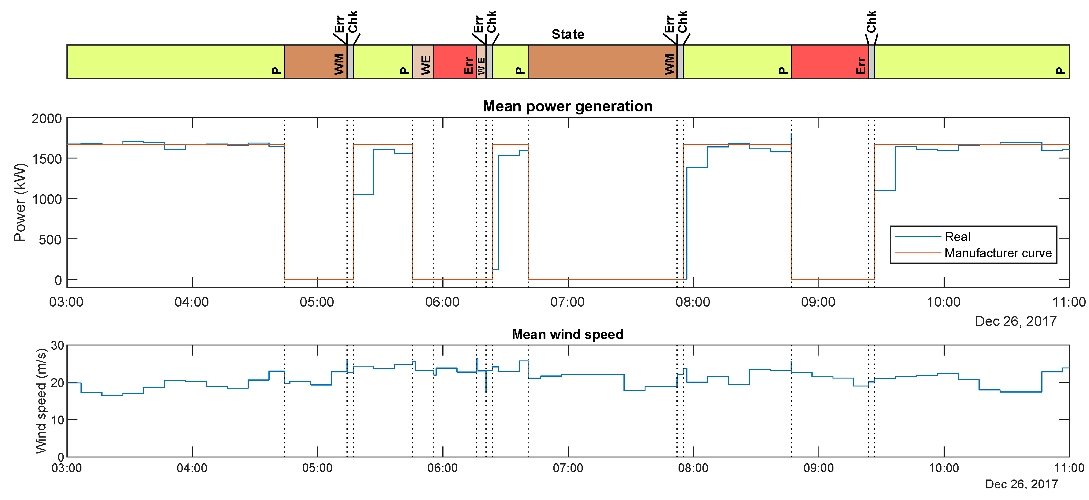This notwithstanding, the transition between PRODUCTION and any other state followed the behavior described by the STOPPING of the simple model, by the equation of Table 3. Every state required a different attention and/or operation by the SCADA users, so this information was valuable to help them in their learning process. Thus, as an example, some interesting cases of the above ones were selected to understand these operational states and their relationship with the operation of SCADA.

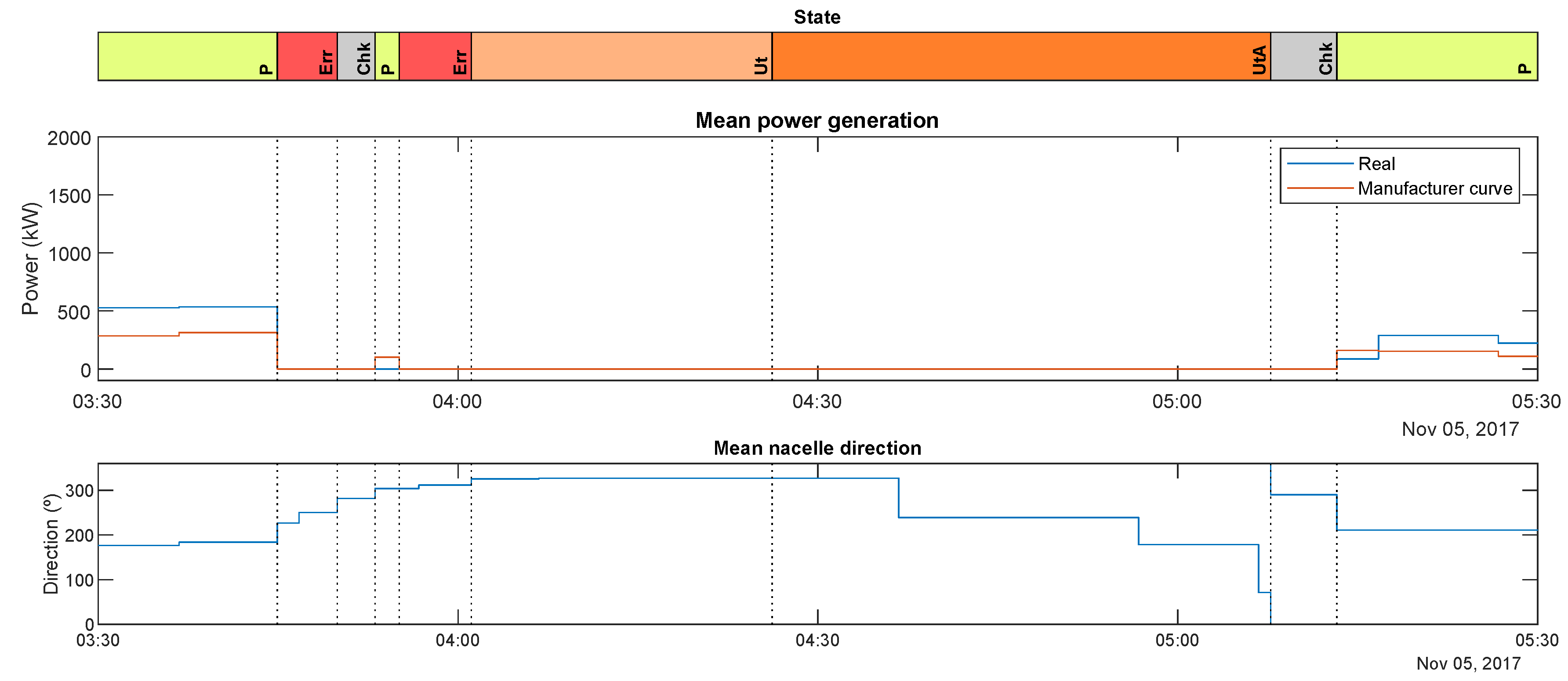
The first one (Figure 14) corresponded to the untwisting process anomaly. At 4:01:06, the turbine started the untwisting process, but as can be seen, the nacelle direction did not change. This was due to an anomaly in the rotation process. Therefore, after 25 min, the system entered the state UNTWISTING ANOMALY (because the angle practically did not change in that period). After some minutes, the system finally achieved rotating, and the system returned to the state PRODUCTION.

When a untwisting anomaly happens, the SCADA operator has the task of finding the cause and solving it. In this case, the operator should check the registered alarms and errors and should choose a corrective maintenance to perform. This process can be appreciated in Figure 15.

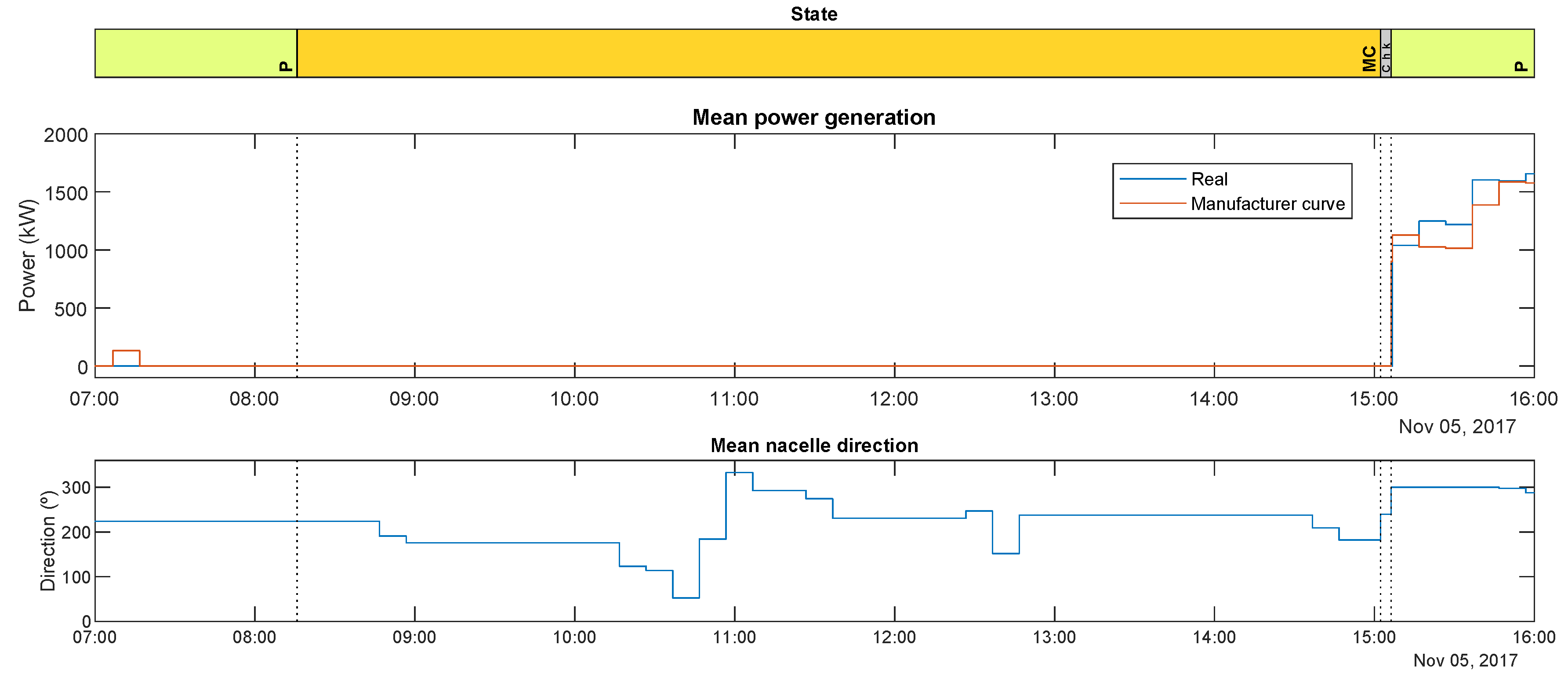
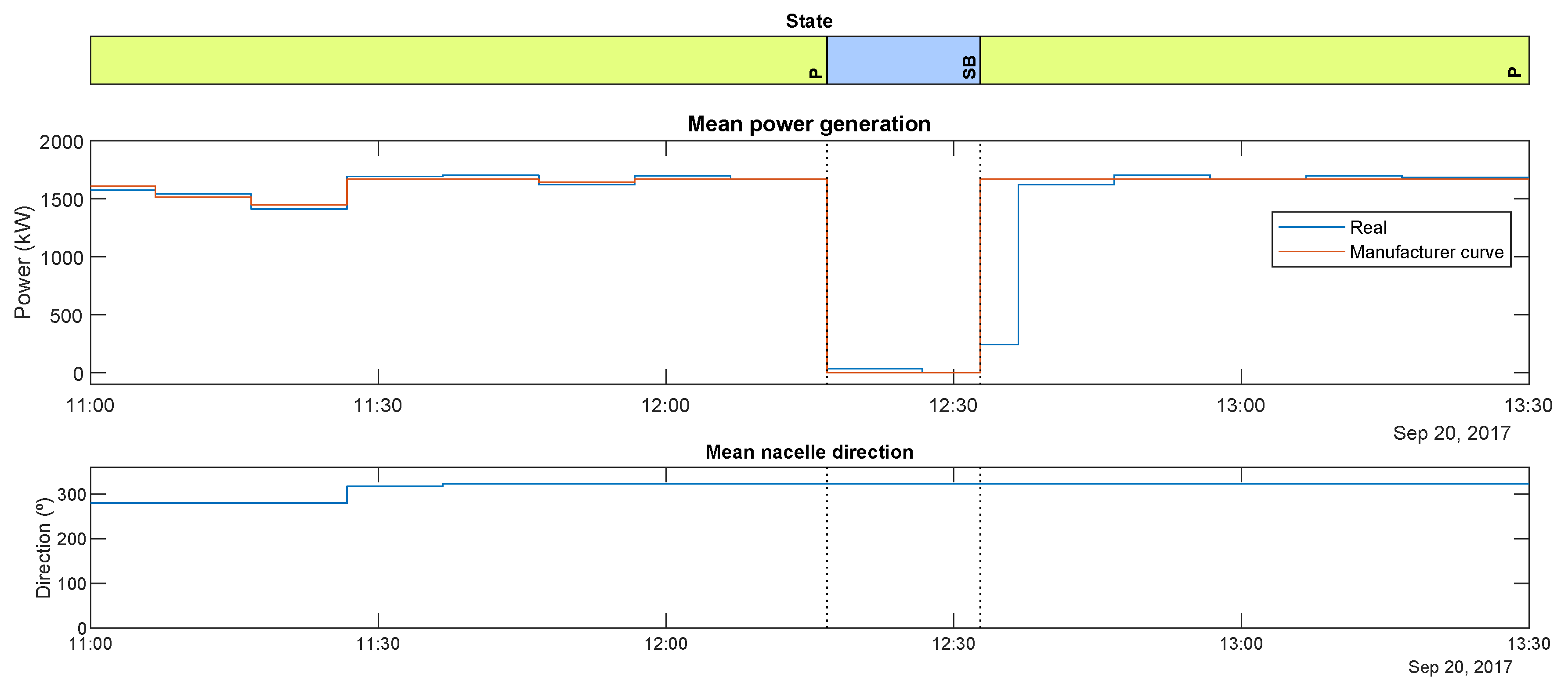
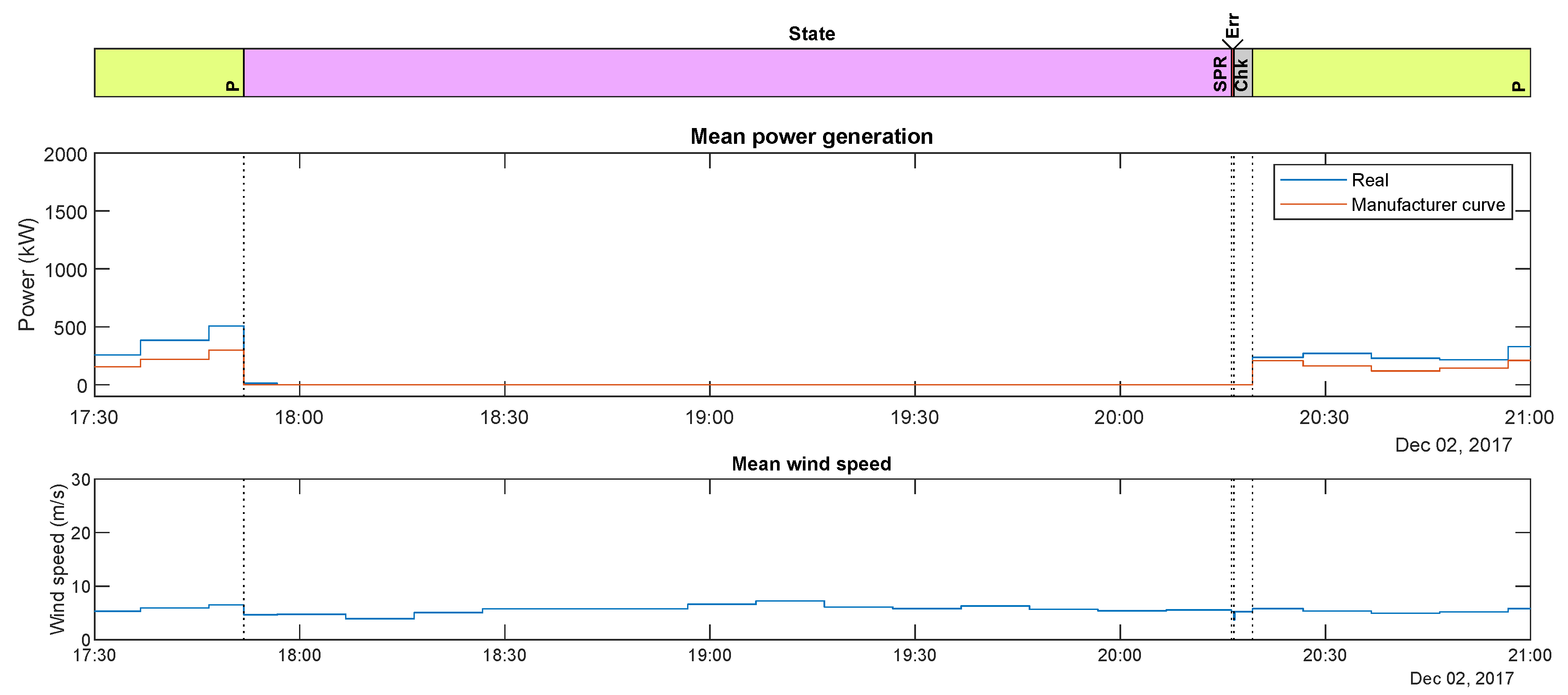
Regarding the stopping of the turbine, there are some reasons for this to occur. Specifically, the three main reasons are: the stop due to birds passing (state STOP-BIRDS), the stop order by the Balance Responsible Parties (BRP) or Independent System Operator (ISO) due to power regulation (state STOP-POWER REGULATION), and the manual stop directly performed by the operator (state MANUAL STOP).

In this sense, Figure 16 shows an event of stopping for birds passing through the zone. Besides, Figure 17 shows a stop case for power regulation from a BRP. The production during the stop time was equal to zero, even with adequate wind speed for power production.

Regarding the normal operation of the wind turbines, the automation system was programmed to avoid damages caused by excessive wind. This was done thanks to the states EXCESSIVE WIND (this happened when the wind speed was more than 25 m/s during a few seconds) and MAXIMUM GUST (when very fast wind gusts were detected). As can be seen in Figure 18, both states could occur during a windy day, and they were important for training purposes.

Additionally, some examples of common errors that could cause the error state are included in

Table 6. List of possible control system errors.

Error Type
Inverter failure
Inverter communication failure
Pitch failure
Pitch communication error
Blade 1 error
Blade 2 error
Blade 3 error

.

Of course, the movement from one state to another required a few signals (some of them depended on the element under control itself, and others depended on the operator actions, being therefore important in training scenarios). They are summarized in

Table 7. List of possible control system signals.

Signal Type	Signal Name	From
Failure	Error Detected	Internal Error
Stop	Stop-Birds	Operator
Stop	Stop-Manual	Operator
Stop	Stop-Power Regulation	Independent System Operator
Maintenance	Maintenance-Corrective	Operator
Maintenance	Maintenance-Preventive	Operator
Maintenance	Maintenance-Programmed	Operator

.

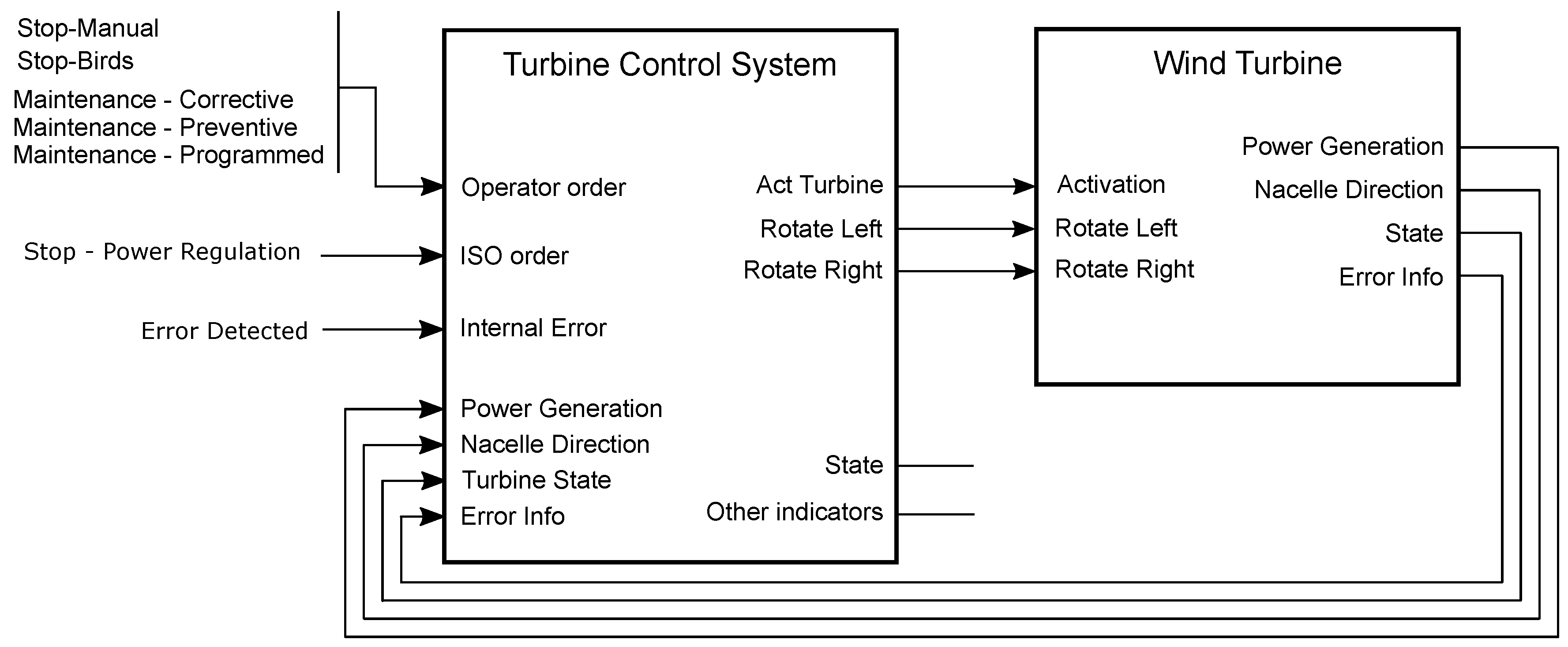
Considering all of the above, the proposed model structure for the control system is shown in Figure 19. As can be seen, it used an extension of the turbine model described above, adding the nacelle control and its associated states.

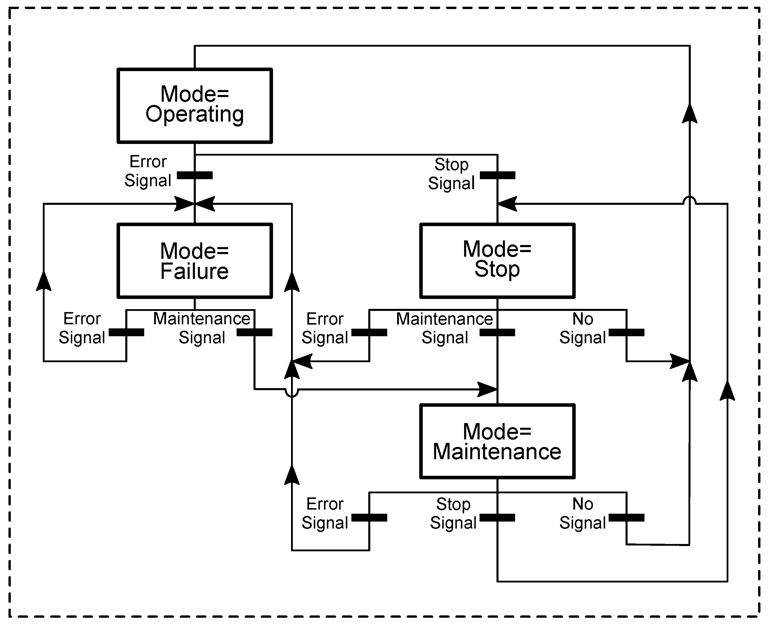
Once all the signals and connections were defined, the states of the control system were implemented in a model for the proposed simulator. This model was done using a double structure: mode and state. The modes (also called procedures) of operation were “global” groups of states, while the states described more specifically how the control system managed the turbine (as listed in Table 5), offering a clear vision of the model and simplifying the model implementation. The summary for this structure is depicted in Figure 20.

The relationship between procedures and the signals that produce an evolution between them are shown in the DES model of Figure 21.

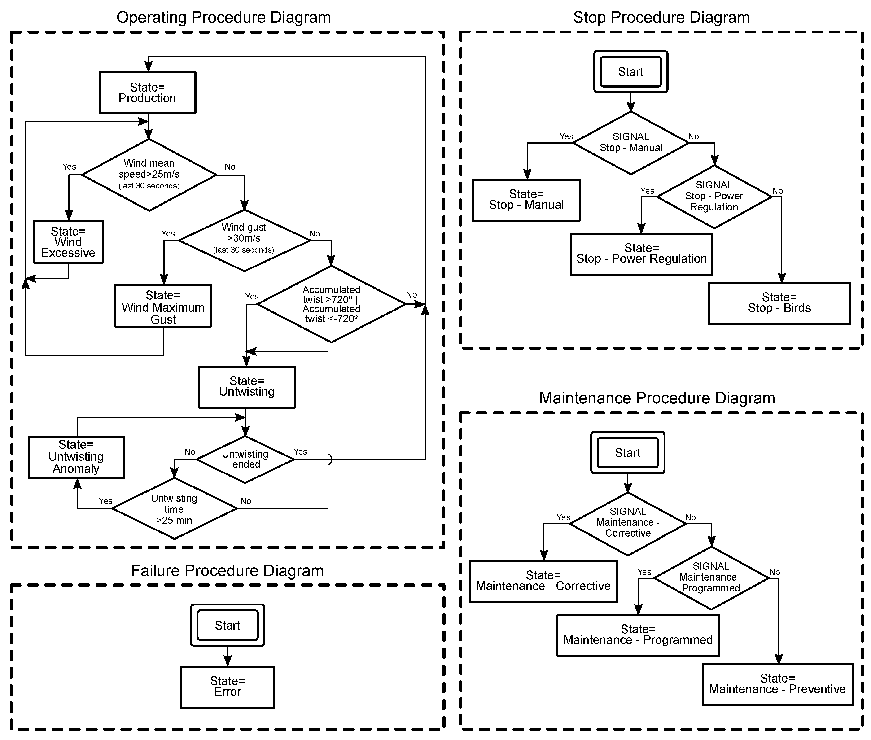
Thus, in each simulation cycle, after deciding the current mode, the DES would be evaluated (see Figure 22). Specifically, the result of this evaluation would be the current state, which would characterize its specific behavior (described above in Table 5).

This proposed model was particularly interesting for the operator training process. Especially, some of the most important states were the stop states, the untwisting anomaly, and errors, which required an operator intervention to check the system and/or a quick response from them, in order to restore the normal turbine operation. In summary, as was explained previously, the actions that a SCADA operator could practice in a simulated scenario using this model were:

Corrective maintenance	Birds stop
Manual stop	Predictive maintenance
Programmed maintenance

Thus, based on the proposed model, the information observed by the operator would be the generation power, the list of errors (if any), and the information about the environment (wind speed and direction).

6. Conclusions

As described before, the presence of renewable generation systems within the energy mix is increasing. However, due to the enormous variability and uncertainty associated with this type of resource, they require sophisticated planning tools in order to manage these resources in a proper way.

Throughout this paper, different examples of the simulation use in the field of the renewable energy were exposed. Nevertheless, these solutions are traditionally focused on the simulation of the generation process or on the facilities’ design, leaving the operation of these systems in the background. Conversely, the need for simulation tools that help to operator in the improvement training and setting task was clearly identified.

In this sense, this paper proposed the integral design of a simulation tool, which could be easily connected to a real SCADA, making it possible to perform simulation under different scenarios. Unlike other simulation tools, which did not have this feature, the proposed simulator could interact directly with real SCADAs similar to a real installation, the interaction not being appreciable by the users, making training more realistic.

Currently, the simulator supports OPC-UA as a communication interface with SCADAs. Furthermore, the communication mechanisms of the simulation tool were flexible and could be configured depending on each SCADA thanks to the modular architecture in which the simulator was designed.

The simulation was defined based on scripts models, making the simplest programming interface possible. This development was carried out taking into account the skills of typical SCADA administrators and operators and establishing JavaScript as the script programming language, easier to learn and being closest to their profile.

As a proof of the usefulness of the proposed tool, a series of possible simulated input data sources for renewable energy simulations was briefly described. In addition, renewable DER models (wind power, PV, and storage systems) were also presented, showing the potential of the proposed simulator.

Additionally, a study case was depicted. Specifically, this study case contained three examples of a wind farm simulation model. A simple one was based on the generation curve given by the manufacturer which only had three states: stop, production, and stopping. Another one was based on empirical data using a recent proposed modeling technique: monotonic splines. A third one had different states and control signals, emulating a more realistic wind turbine system, being more useful in the operator training process.

As can be seen from the script examples, the proposed programming language and the provided API were simple. Thanks to this, plant administrators could create new simulation scenarios, without needing advanced programming skills. Thus, these models would allow them to sort out that which is lacking as typically detected in the support of renewable SCADAs, such as: setting up facilities or the training of novel operators.