Numerical Study of the Winter–Kennedy Flow Measurement Method in Transient Flows

Abstract
1. Introduction
2. Methods
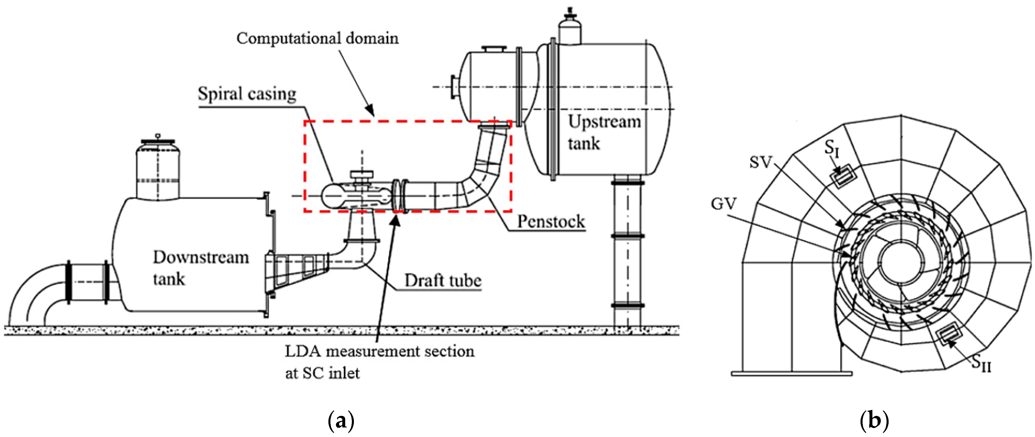
2.1. Porjus U9 Model Test Case and the Computational Domain
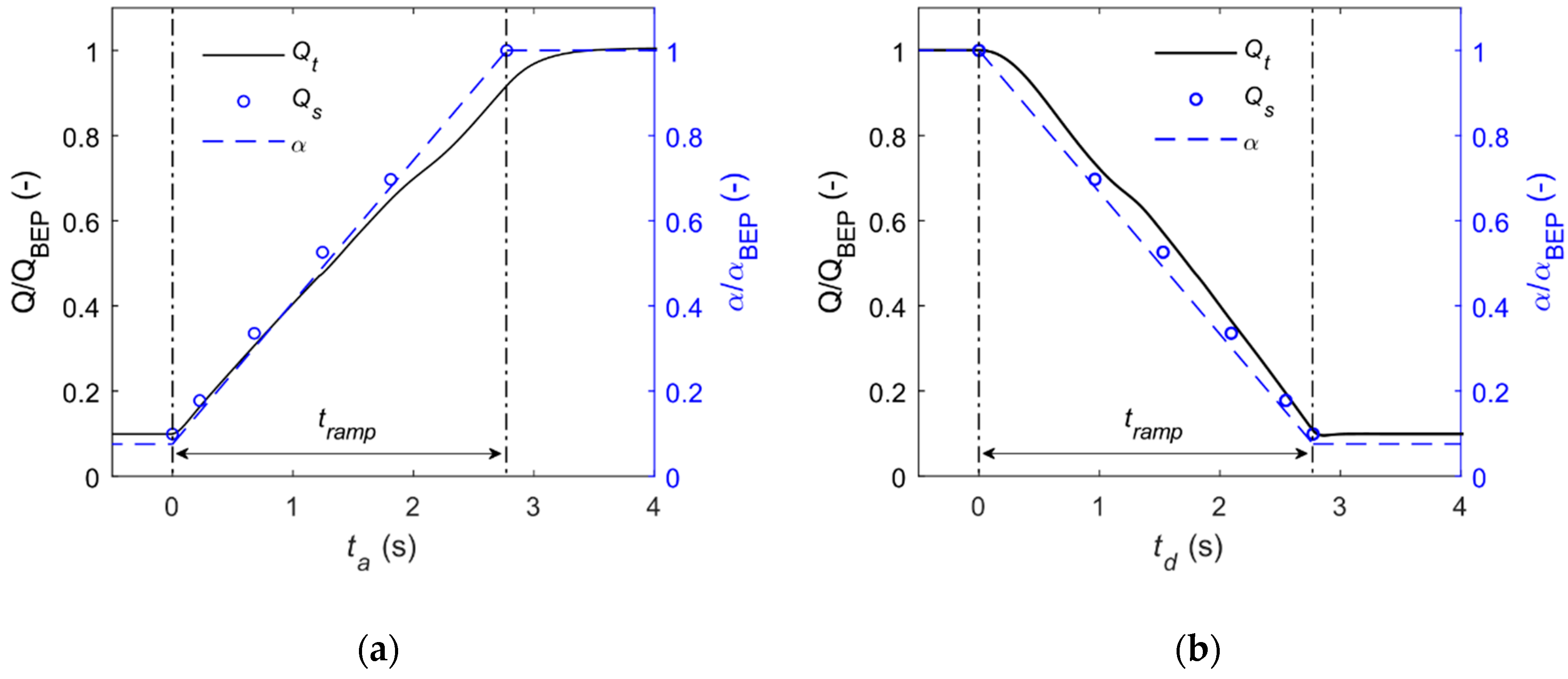
2.2. Transient Cases
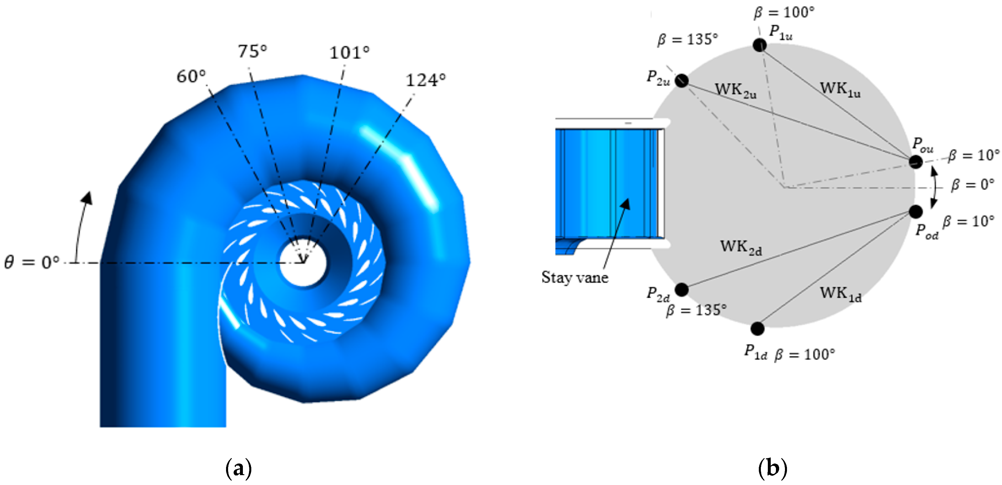
2.3. WK Configurations and Locations
2.4. Numerical Approach
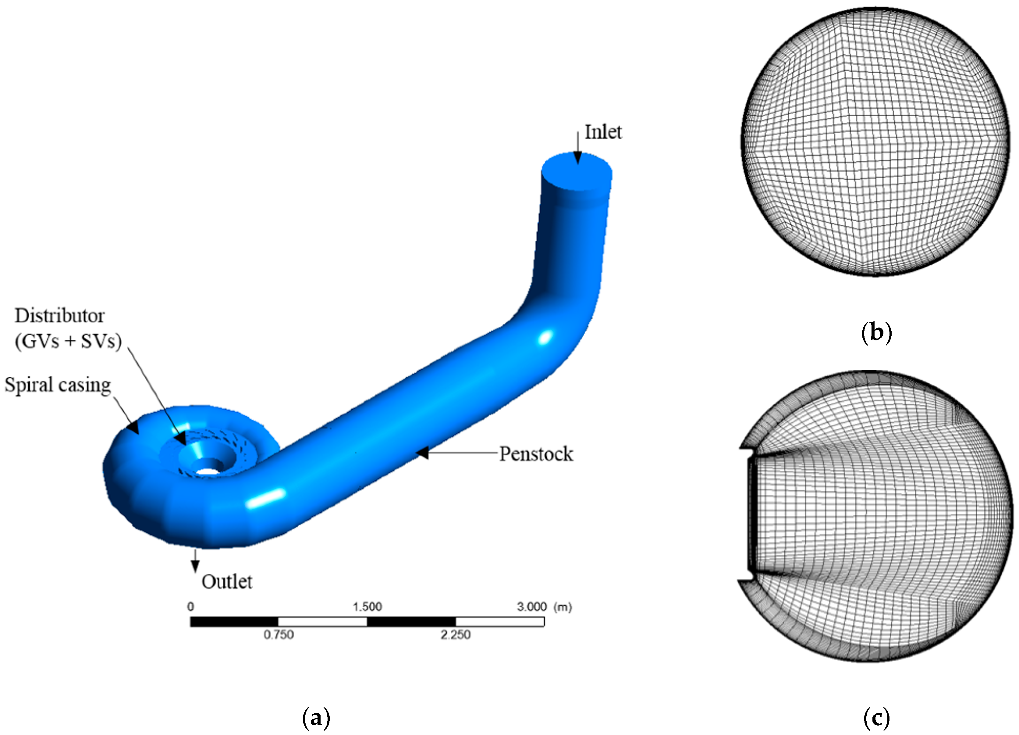
2.4.1. Computational Domain
2.4.2. Guide Vanes Motion
2.4.3. Governing Equations and Boundary Conditions
2.4.4. Mesh Information and Numerical Uncertainties
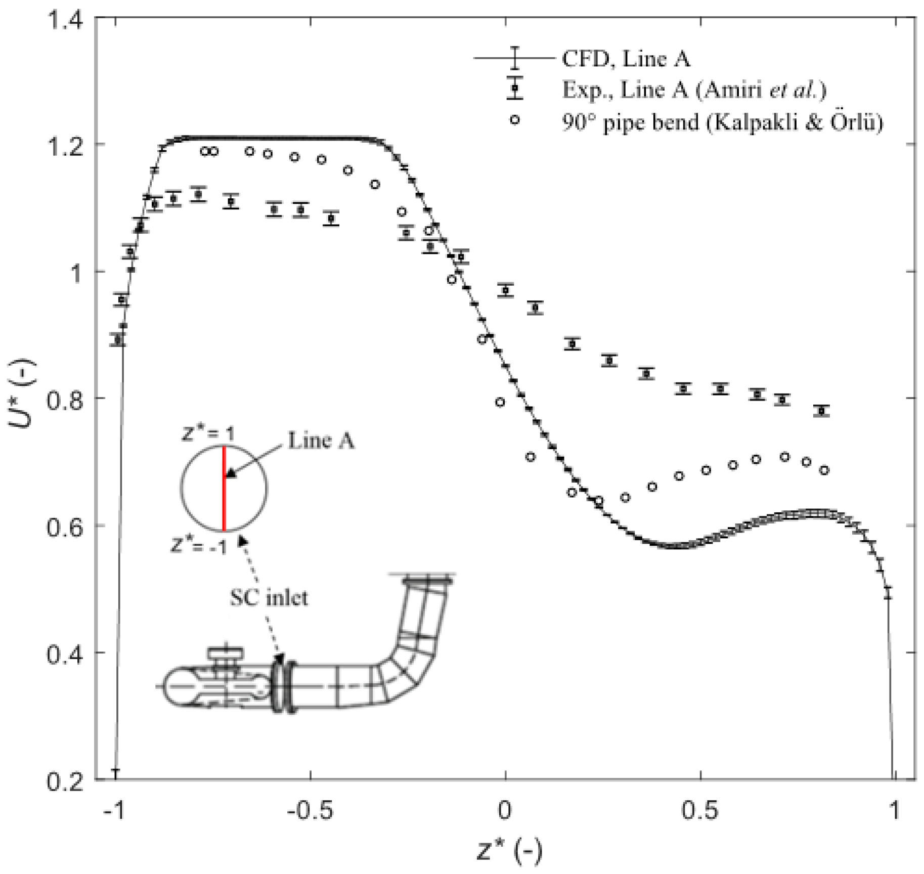
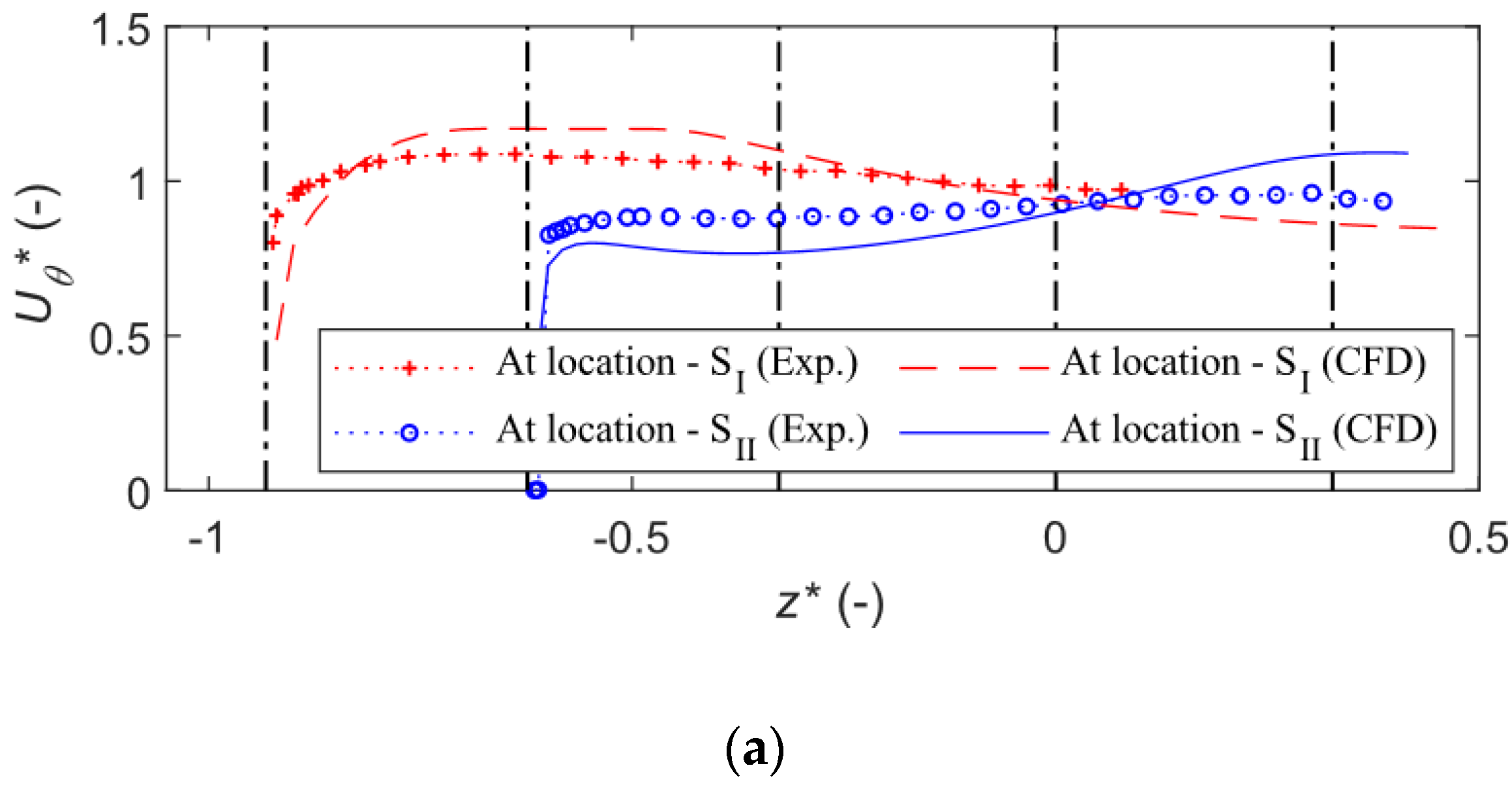
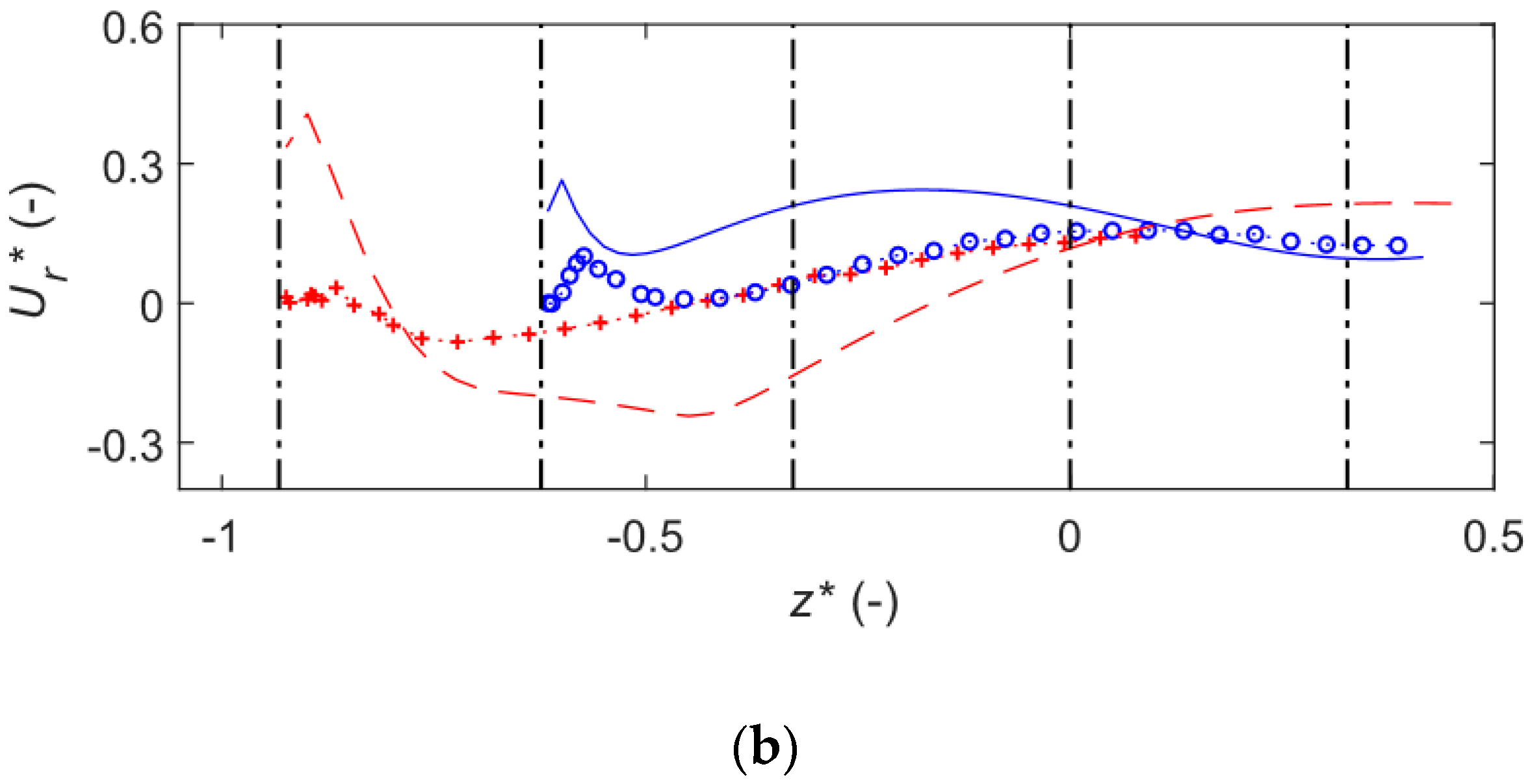
2.4.5. Validation Studies
3. Results
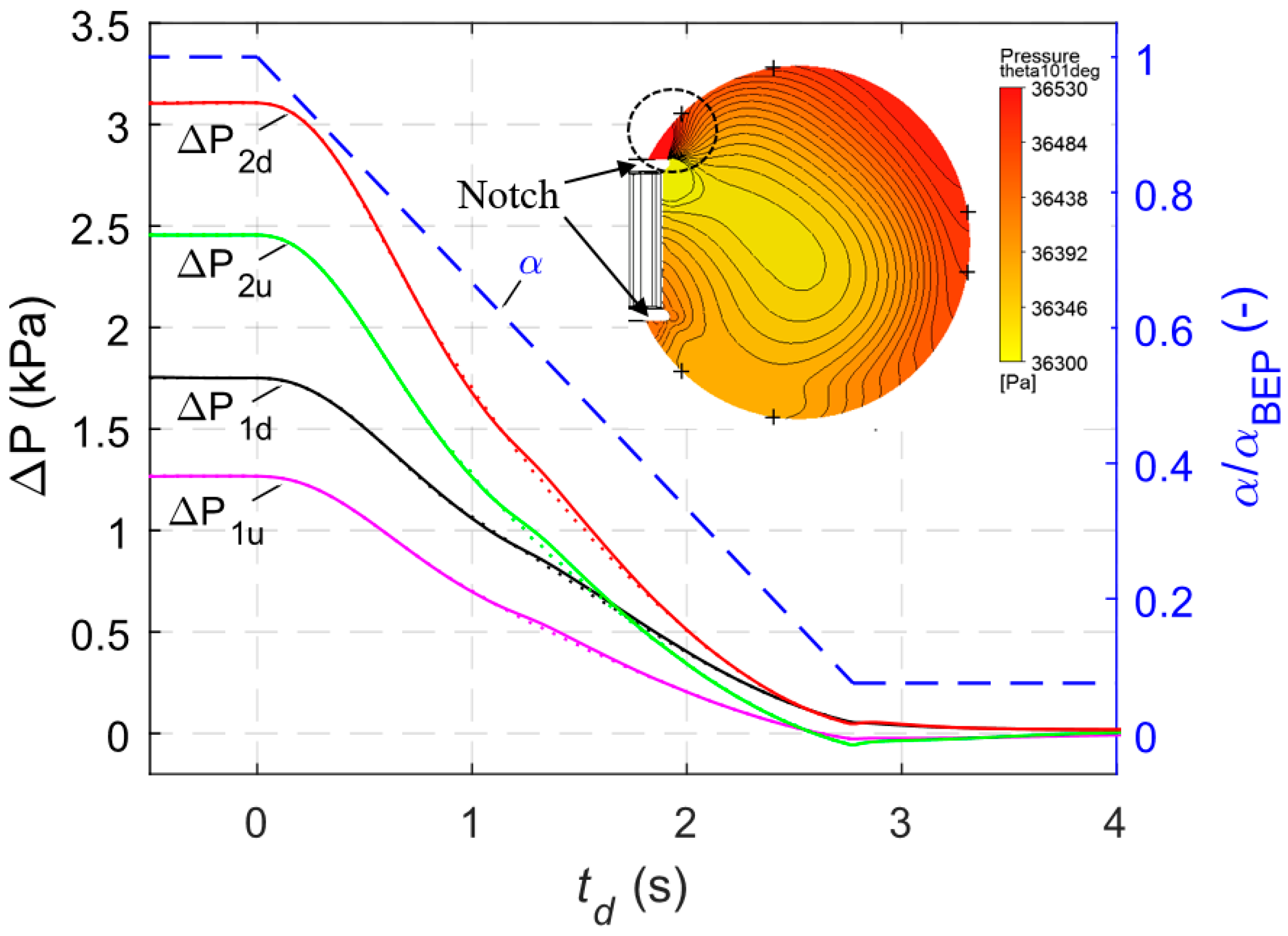
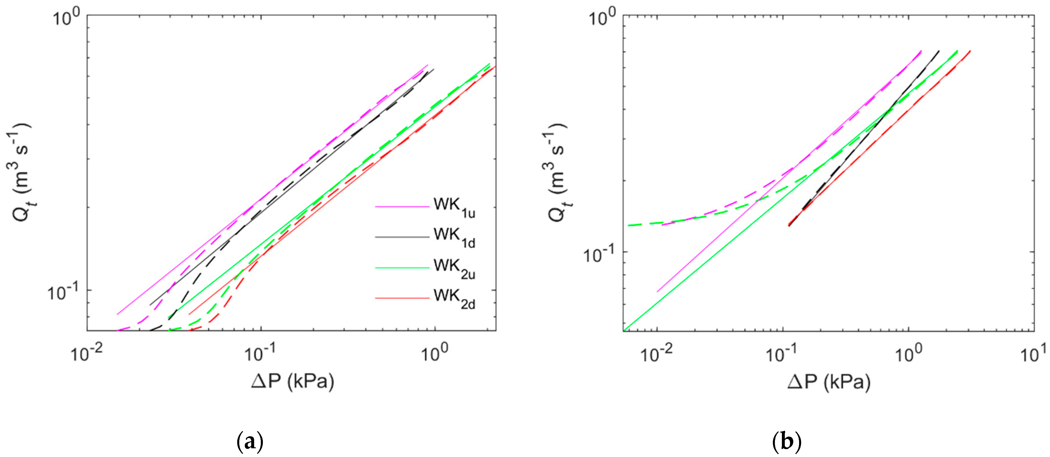
3.1. Variation of Pressure Difference ∆P and Flow Rate
3.2. Variations of the WK Coefficients During Transients
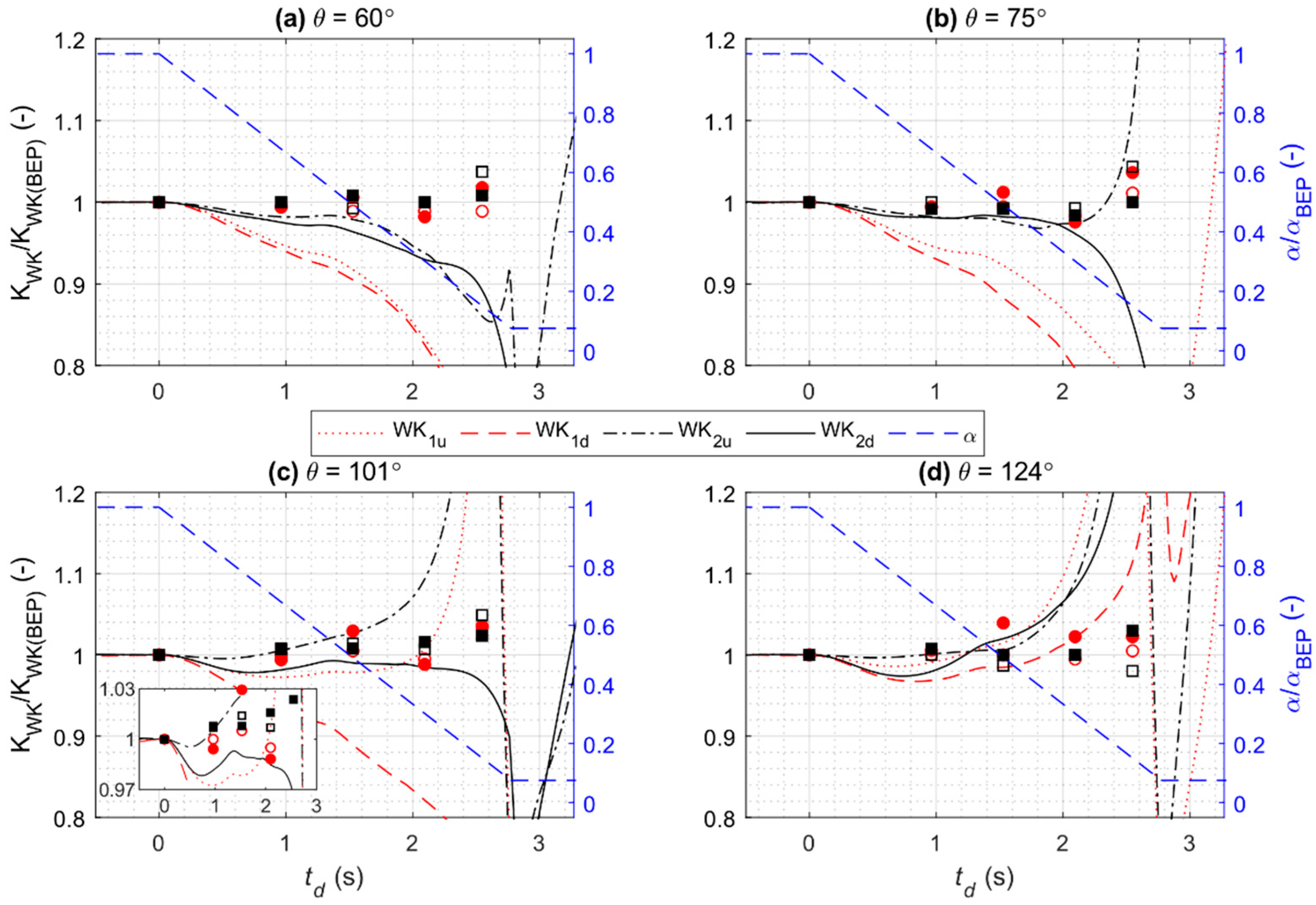
3.2.1. Decelerating Flow
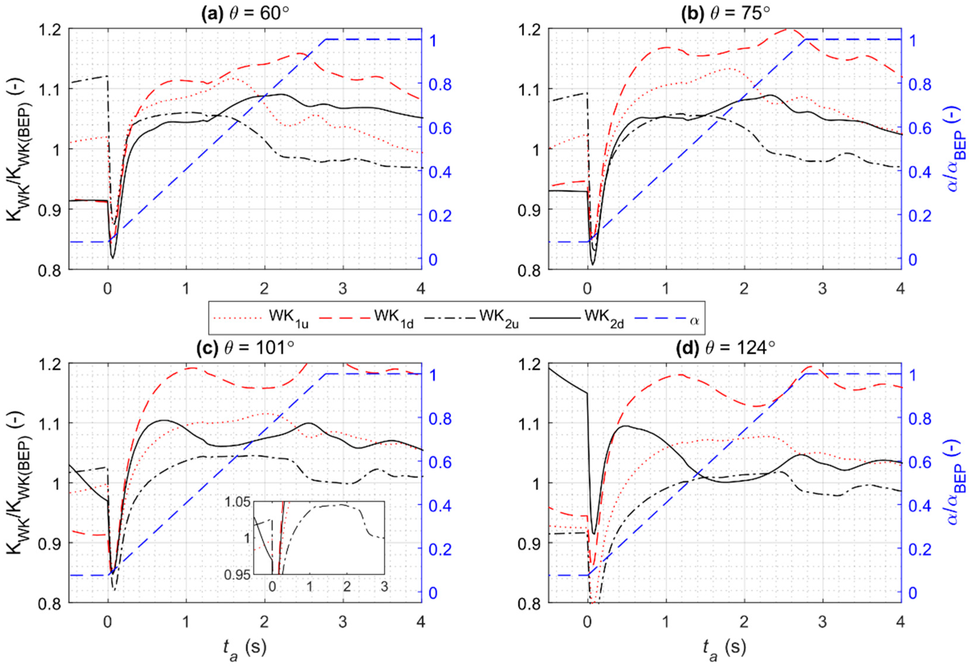
3.2.2. Accelerating Flow
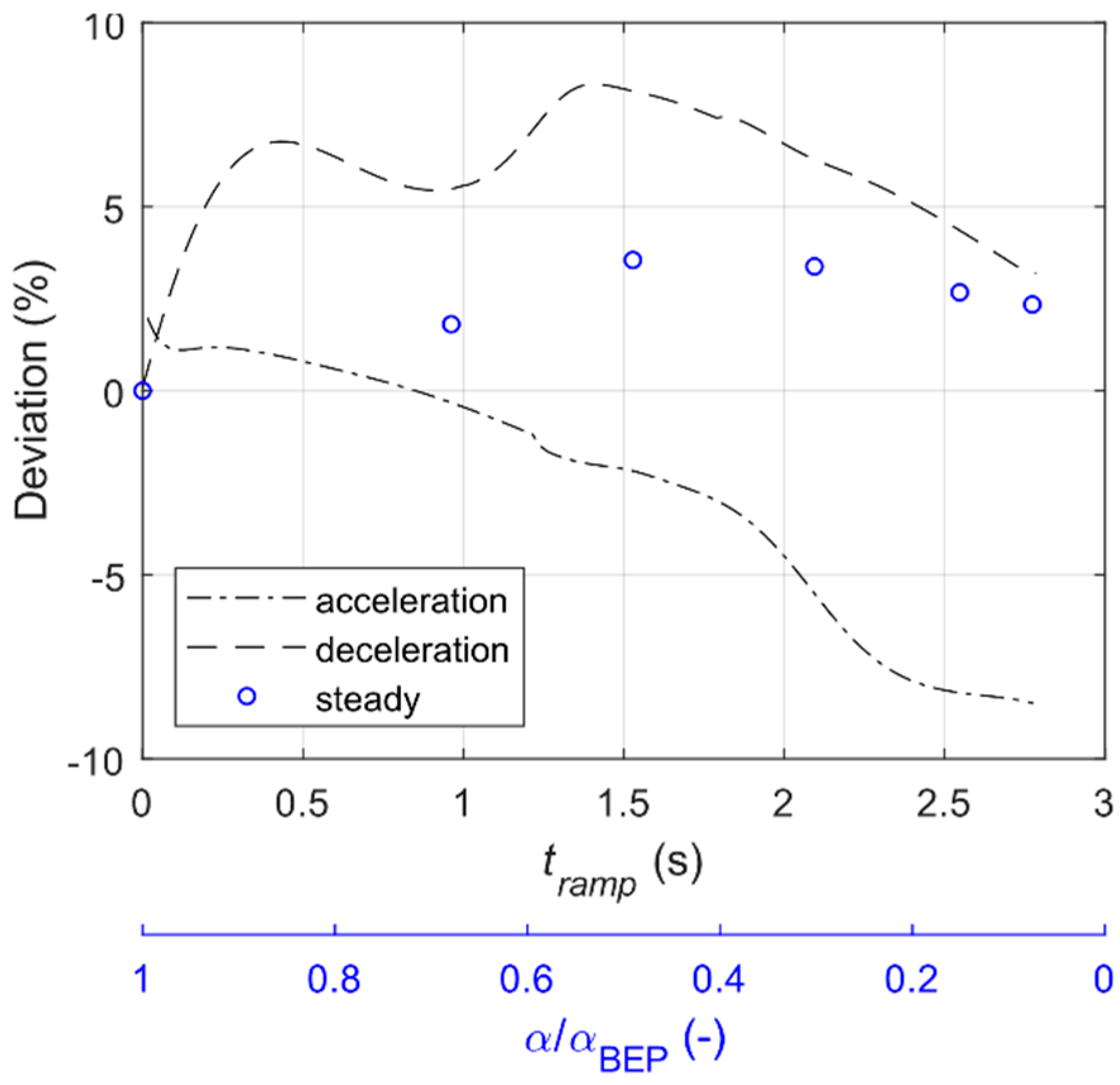
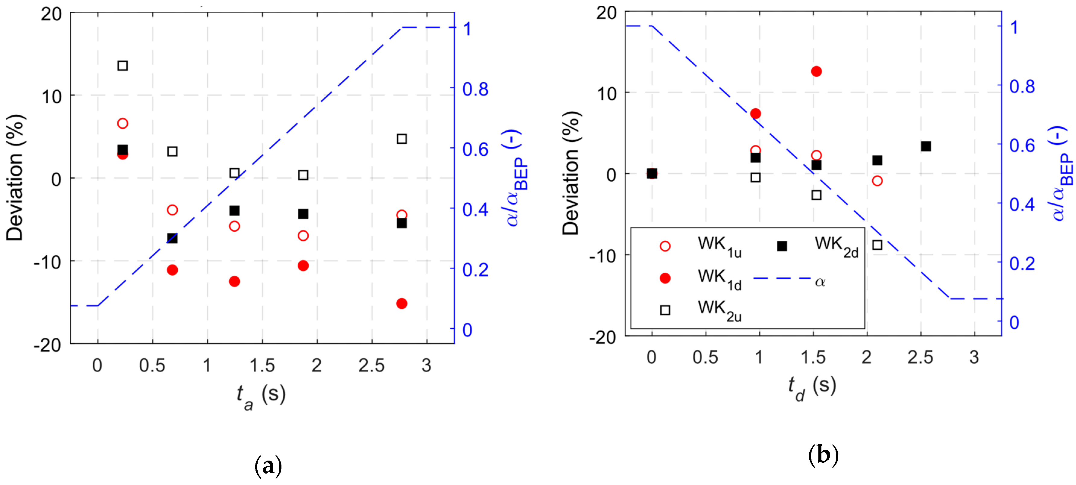
3.3. Practical Use of the WK Method in Transients
3.4. Flow Physics
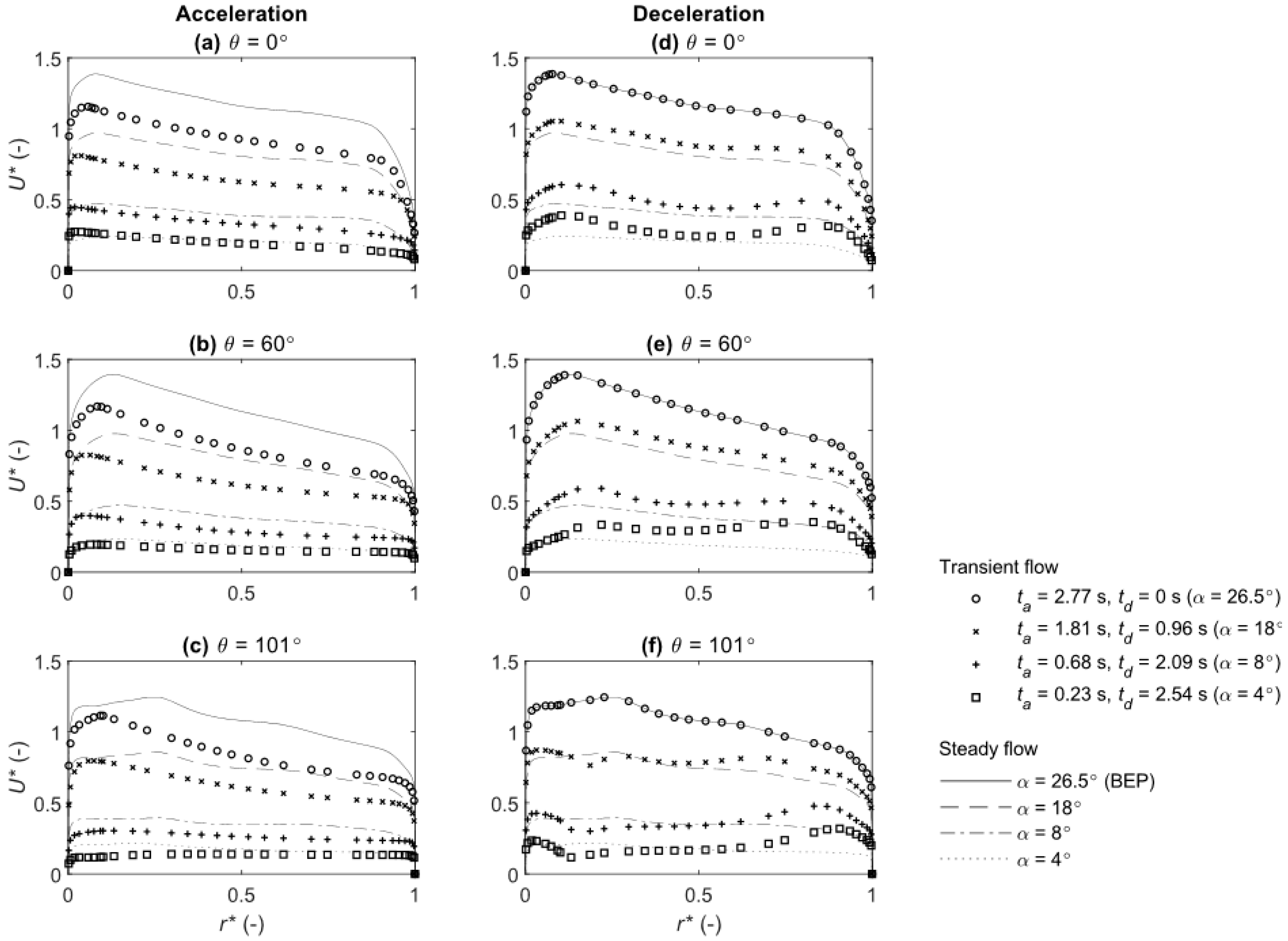
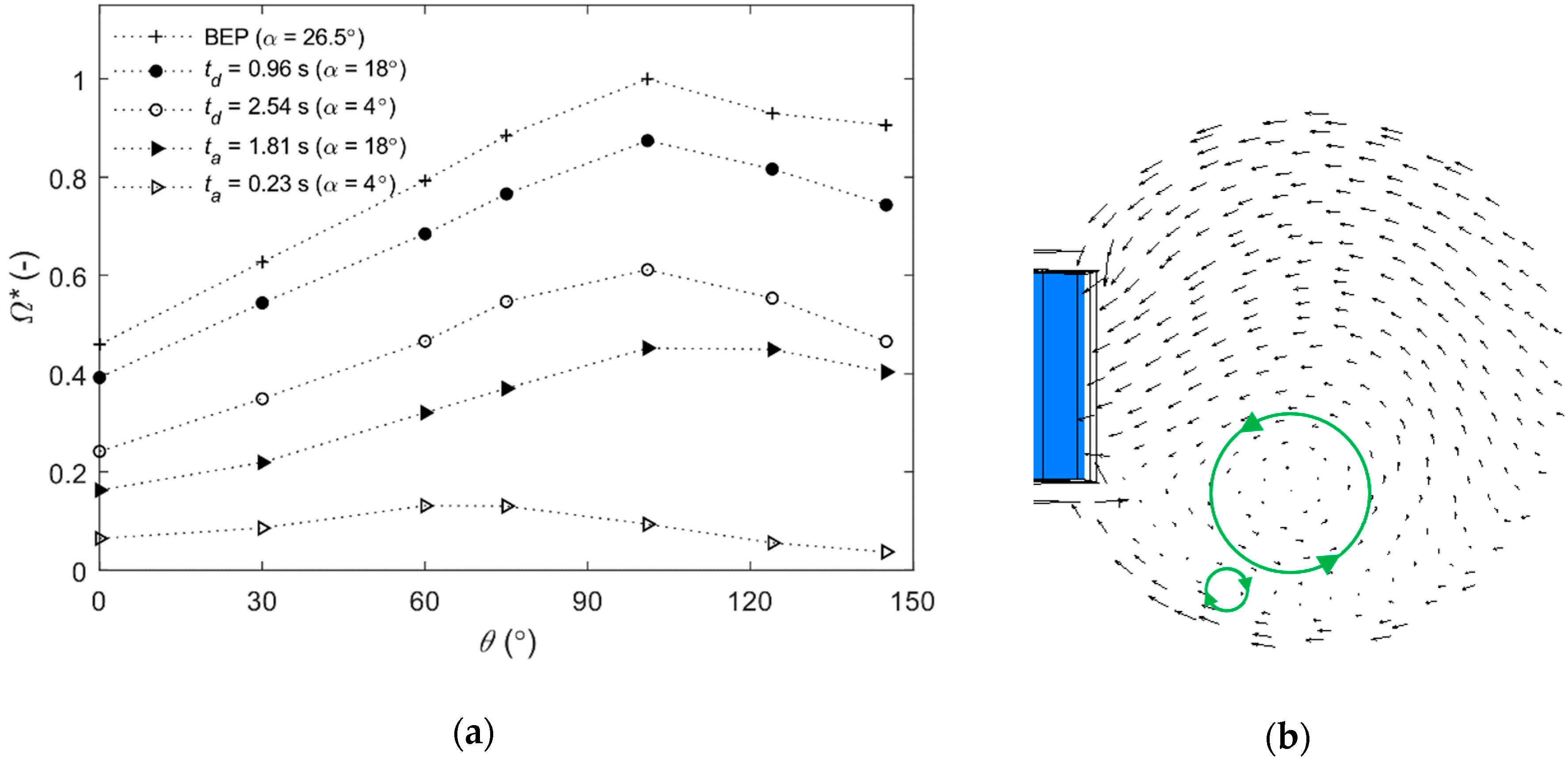
3.4.1. Velocity and Vorticity Development
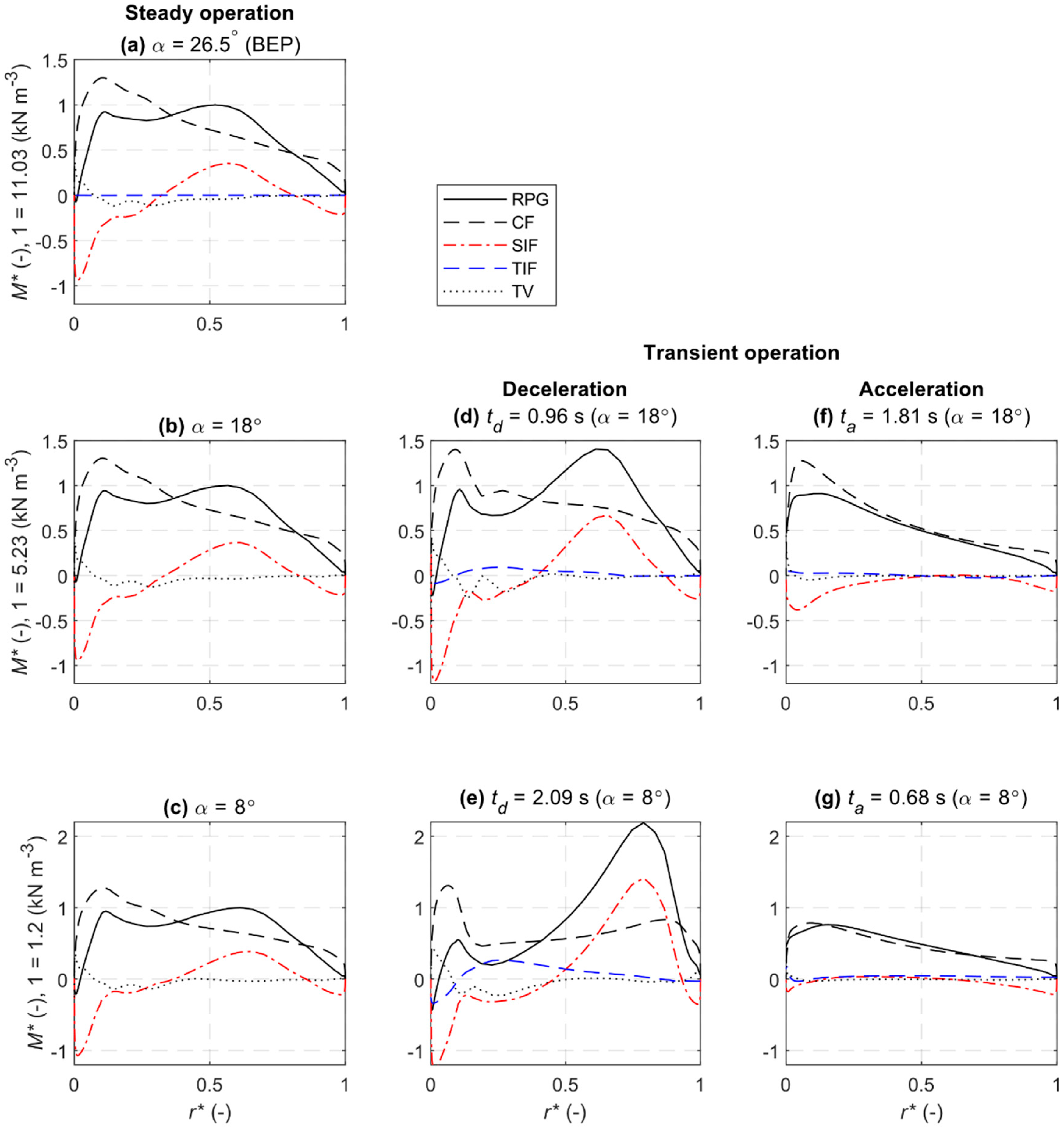
3.4.2. Turbulence, Secondary Flow, and Temporal Forces
4. Conclusions
Author Contributions
Funding
Acknowledgments
Conflicts of Interest
Nomenclature
| inlet area of the spiral casing (SC), m2 | |
| penstock diameter at the inlet of the spiral casing, m | |
| WK coefficient, m3.5/kg0.5 | |
| WK coefficient obtain at BEP flow condition (steady), m3.5/kg0.5 | |
| WK exponent | |
| number of mesh elements in fine, medium and coarse mesh | |
| pressure difference between outer and inner WK pressure points, Pa | |
| flow rate (discharge), m3/s | |
| flow rate (steady) at BEP, m3/s | |
| estimated flow rate using and , m3/s | |
| steady flow rate obtained at stationary , m3/s | |
| transient (instantaneous) flow rate, m3/s | |
| difference in the transient and steady flow rate at same | |
| dimensionless radial distance | |
| time, s | |
| time step, s | |
| accelerating time (transient time), s | |
| decelerating time (transient time), s | |
| the time when the transient starts, s | |
| bulk velocity calculated at the SC inlet at BEP, m3/s | |
| streamwise velocity (total), m/s | |
| tangential velocity, m/s | |
| radial velocity, m/s | |
| dimensionless wall distance | |
| dimensionless vertical distance in the spiral casing, m | |
| Greek Symbols | |
| guide vane angle, ° | |
| time step in terms of guide vane rotation angle, ° | |
| circumferential location/azimuthal angle of the SC, ° | |
| density of the fluid (water), kg/m3 | |
| total vorticity | |
References
- Trivedi, C.; Gandhi, B.K.; Cervantes, M.J. Effect of transients on Francis turbine runner life: A review. J. Hydraul. Res. 2013, 51, 121–132. [Google Scholar] [CrossRef]
- Siemonsmeier, M.; Baumanns, P.; Bracht, N.V.; Schönefeld, M.; Schönbauer, A.; Moser, A.; Dahlhaug, O.G.; Heidenreich, S. Hydropower Providing Flexibility for a Renewable Energy System: Three European Energy Scenarios—A HydroFlex Report; HydroFlex: Trondheim, Norway, 2018. [Google Scholar]
- Iliev, I.; Trivedi, C.; Dahlhaug, O.G. Variable-speed operation of Francis turbines: A review of the perspectives and challenges. Renew. Sustain. Energy Rev. 2019, 103, 109–121. [Google Scholar] [CrossRef]
- International Electrotechnical Commission. IEC-60193Hydraulic Turbines, Storage Pumps and Pump-Turbines—Model Acceptance Tests; International Electrotechnical Commission: Geneva, Switzerland, 1999. [Google Scholar]
- International Standard. IEC 60041Field Acceptance Tests to Determine the Hydraulic Performance of Hydraulic Turbines, Storage Pumps and Pump Turbines; International Standard: Geneva, Switzerland, 1991. [Google Scholar]
- ASME. PTC-18 Performance Test Code 18: Hydraulic Turbines and Pump-Turbines; ASME: New York, NY, USA, 2002. [Google Scholar]
- Almquist, C.W.; Taylor, J.W.; Walsh, J.T. Kootenay Canal Flow Rate Measurement Comparison Test Using Intake Methods; HydroVision: Sacramento, CA, USA, 2011. [Google Scholar]
- Taylor, J.; Proulx, G.; Lampa, J. Turbine Flow Measurement in Intakes—A Cost-Effective Alternative to Measurement in Penstocks; Hydro: Prague, Czech Republic, 2011. [Google Scholar]
- Leontidis, V.; Cuvier, C.; Caignaert, G.; Dupont, P.R.O.; Fammery, S.; Nivet, P.; Dazin, A. Experimental validation of an ultrasonic flowmeter for unsteady flows. Meas. Sci. Technol. 2018, 29, 045303. [Google Scholar] [CrossRef]
- Cheesewright, R.; Clark, C.; Hou, Y.Y. The response of Coriolis flowmeters to pulsating flows. Flow Meas. Instrum. 2004, 15, 59–67. [Google Scholar] [CrossRef]
- Lefebvre, P.J.; Durgin, W.W. A Transient Electromagnetic Flowmeter and Calibration Facility. J. Fluids Eng. 1990, 112, 12–15. [Google Scholar] [CrossRef]
- Fraser, R.; Coulaud, M.; Aeschlimann, V.; Lemay, J.; Deschênes, C. Method for experimental investigation of transient operation on Laval test stand for model size turbines. In IOP Conference Series Earth and Environmental Science; IOP: Bristol, UK, 2016; Volume 49, p. 062006. [Google Scholar] [CrossRef]
- Trivedi, C.; Cervantes, M.J.; Gandhi, B.K.; Dahlhaug, O.G. Transient pressure measurements on a high head model Francis turbine during emergency shutdown, total load rejection, and runaway. J. Fluids Eng. 2014, 136, 121107. [Google Scholar] [CrossRef]
- Amiri, K.; Mulu, B.; Mehrdad, R.; Cervantes, M.J. Unsteady pressure measurements on the runner of a Kaplan turbine during load acceptance and load rejection. J. Hydraul. Res. 2015, 54, 56–73. [Google Scholar] [CrossRef]
- He, S.; Jackson, J.D. A study of turbulence under conditions of transient flow in a pipe. J. Fluid Mech. 2000, 408, 1–38. [Google Scholar] [CrossRef]
- He, S.; Ariyaratne, C.; Vardy, A. A computational study of wall friction and turbulence dynamics in accelerating pipe flows. Comput. Fluids 2008, 37, 674–689. [Google Scholar] [CrossRef]
- Sundstrom, J.L.R.; Cervantes, M.J. Laminar similarities between accelerating and decelerating turbulent flows. Int. J. Heat Fluid Flow 2018, 71, 13–26. [Google Scholar] [CrossRef]
- He, S.; Seddighi, M. Turbulence in transient channel flow. J. Fluid Mech. 2013, 715, 60–102. [Google Scholar] [CrossRef]
- Seddighi, M.; Shuisheng, H.; Orlandi, P. A Comparative Study of Turbulence in Ramp-Up and Ramp-Down Unsteady Flows. Flow Turbul. Combust. 2011, 86, 439–454. [Google Scholar] [CrossRef]
- Gorji, A.; Seddighi, M.; Ariyaratne, C.; Vardy, A.E.; O’Donoghue, T.; Pokrajac, D.; He, S. A comparative study of turbulence models in a transient channel flow. Comput. Fluids. 2014, 89, 111–113. [Google Scholar] [CrossRef]
- Ariyaratne, C.; He, S.; Vardy, A.E. Wall friction and turbulence dynamics in decelerating pipe flows. J. Hydraul. Res. 2010, 48, 810–821. [Google Scholar] [CrossRef]
- Winter, I.A.; Kennedy, A.M. Improved type of flow meter for hydraulic turbines. ASCE Proc. 1933, 59, 4. [Google Scholar]
- Isaksson, H.; Sendelius, M.; Cervantes, M.J. Cam curve in Kaplan turbine, a sensitivity analysis. UPB Sci. Bull. Ser. D 2016, 78, 185–192. [Google Scholar]
- Lövgren, M.H.; Andersson, U.; Andrée, G. Skew Inlet Flow in a Model Turbine-Effects on Winter–Kennedy Measurements; Hydro: Ljubljana, Slovenia, 2008. [Google Scholar]
- Baidar, B.; Nicolle, J.; Gandhi, B.K.; Cervantes, M.J. Numerical study of the Winter–Kennedy method for relative transient flow rate measurement. In IAHR International Workshop on Cavitation and Dynamic Problems in Hydraulic Machinery and Systems, Stuttgart; IOP Conference Series Earth and Environmental Science; IOP Publishing: Bristol, UK, 2019; Volume 405, p. 012022. [Google Scholar] [CrossRef]
- Amiri, K.; Mulu, B.; Raisee, M.; Cervantes, M.J. Effects of upstream flow conditions on runner pressure fluctuations. J. Appl. Fluid Mech. 2017, 10, 1045–1059. [Google Scholar] [CrossRef]
- Mulu, B.G.; Cervantes, M.J. LDA measurements in a Kaplan spiral casing model. In 13th Symposium on Transport Phenomena and Dynamics of Rotating Machinery; Curran Associates, Inc.: Honolulu, HI, USA, 2010. [Google Scholar]
- Mössinger, P.; Jester-Zürker, R.; Jung, A. Francis-99: Transient CFD simulation of load changes and turbine shutdown in a model sized high-head Francis turbine. In IOP Conference Series: Journal of Physics; IOP Publishing: Bristol, UK, 2017; Volume 782, p. 012001. [Google Scholar] [CrossRef]
- Nicolle, J.; Morissette, J.F.; Giroux, A.M. Transient CFD simulation of a Francis turbine startup. In IOP Conference Series: Earth and Environmental Science; IOP Publishing: Bristol, UK, 2012; Volume 15, p. 062014. [Google Scholar] [CrossRef]
- ANSYS, Inc. CFX—Solver Theory Guide 19.1; ANSYS, Inc.: Canonsburg, PA, USA, 2019. [Google Scholar]
- Menter, F. Two-Equation Eddy-Viscosity Turbulence Models for Engineering Applications. AIAA J. 1994, 32, 1598–1605. [Google Scholar] [CrossRef]
- Mössinger, P.; Zürker-Jester, R.; Jung, A. Investigation of different simulation approaches on a high-head Francis turbine and comparison with model test data: Francis-99. J. Phys. IOP Conf. Ser. 2015, 579, 012005. [Google Scholar] [CrossRef]
- Chen, H.; Zhou, D.; Zheng, Y.; Jiang, S.; Yu, A.; Guo, Y. Load rejection transient process simulation of a Kaplan turbine model by co-adjusting guide vanes and runner blades. Energies 2018, 11, 3354. [Google Scholar] [CrossRef]
- Trivedi, C.; Cervantes, M.J.; Dahlhaug, O.G. Numerical Techniques Applied to Hydraulic Turbines: A Perspective Review. Appl. Mech. Rev. 2016, 68, 010802. [Google Scholar] [CrossRef]
- Saemi, S.; Raisee, M.; Cervantes, M.J.; Nourbakhsh, A. Numerical investigation of the Pressure-Time Method considering pipe with variable cross section. J. Fluids Eng. 2018, 140, 101401. [Google Scholar] [CrossRef]
- Saemi, S.; Cervantes, M.J.; Raisee, M.; Nourbakhsh, A. Numerical investigation of the Pressure-time method. Flow Meas. Instrum. 2017, 55, 44–58. [Google Scholar] [CrossRef]
- Celik, I.; Ghia, U.; Roache, P.; Freitas, C.; Coleman, H.; Raad, P. Procedure for Estimation and Reporting of Uncertainty due to Discretization in CFD Applications. J. Fluids Eng. 2008, 130, 078001-(1-4). [Google Scholar] [CrossRef]
- Kalpakli, A.; Örlü, R. Turbulent pipe flow downstream a 90° pipe bend with and without superimposed swirl. Int. J. Heat Fluid Flow 2013, 41, 103–111. [Google Scholar] [CrossRef]
- Vester, A.K.; Örlü, R.; Alfredsson, H. Turbulent Flows in Curved Pipes: Recent Advances in Experiments and Simulations. Appl. Mech. Rev. 2016, 68, 050802. [Google Scholar] [CrossRef]
- Baidar, B.; Nicolle, J.; Gandhi, B.K.; Cervantes, M.J. Sensitivity of the Winter–Kennedy method to different guide vane openings on an axial machine. Flow Meas. Instrum. 2019, 68, 101585. [Google Scholar] [CrossRef]
- Cuming, H.G. The Secondary Flow in Curved Pipes; Aeronautical Research Council: London, UK, 1955. [Google Scholar]
- Hara, K.; Furukawa, M.; Inoue, M. Behavior of three-dimensional boundary layers in a radial inflow turbine scroll. In ASME 1993 International Gas Turbine and Aeroengine Congress and Exposition; American Society of Mechanical Engineers Digital Collection: Cincinnati, OH, USA, 1993. [Google Scholar]
- Boiron, O.; Valérie, D.; Pelissier, R. Experimental and numerical studies on the starting effect on the secondary flow in a bend. J. Fluid Mech. 2007, 574, 109–129. [Google Scholar] [CrossRef]
- Baidar, B.; Nicolle, J.; Trivedi, C.; Cervantes, M.J. Numerical Study of the Winter–Kennedy Method—A Sensitivity Analysis. J. Fluids Eng. 2018, 140, 051103. [Google Scholar] [CrossRef]


| Case | αinitial (°) | αfinal (°) | Ramp Time (s) |
|---|---|---|---|
| Acceleration (GV opening) | 2 | 26.5 | 2.77 |
| Deceleration (GV closing) | 26.5 | 2 | 2.77 |
| Parameter | ||||
|---|---|---|---|---|
| 0.0199 | 0.0170 | 0.0143 | 0.0127 | |
| 0.0196 | 0.0172 | 0.0143 | 0.0125 | |
| 0.0204 | 0.0181 | 0.0145 | 0.0128 | |
| 0.0202 | 0.0168 | 0.0143 | 0.0129 | |
| 1.4% | 1.0% | 0.1% | 1.5% |
| Parameters | Penstock | Spiral Casing | Distributor (SV + GV) | ||
|---|---|---|---|---|---|
| α = 26.5° | α = 18° | α = 8° | |||
| Total elements, in million | 1.4 | 1.8 | 6.4 | 6.4 | 6.4 |
| Max. element aspect ratio | 9200 | 2429 | 416 | 516 | 557 |
| Orthogonality angle, ° (min, avg) | 35, 84 | 19, 65 | 22, 59 | 19, 57 | 19, 56 |
| (avg, max) | 1, 495 | 20, 130 | 19, 224 | 16, 161 | 13, 67 |
| WK | R2 | |||||
|---|---|---|---|---|---|---|
| Acceleration | Deceleration | Acceleration | Deceleration | Acceleration | Deceleration | |
| WK1u | 0.693 | 0.619 | 0.508 | 0.480 | 0.998 | 0.994 |
| WK1d | 0.642 | 0.619 | 0.526 | 0.480 | 0.997 | 0.999 |
| WK2u | 0.465 | 0.468 | 0.500 | 0.443 | 0.997 | 0.993 |
| WK2d | 0.433 | 0.397 | 0.512 | 0.504 | 0.999 | 0.999 |
© 2020 by the authors. Licensee MDPI, Basel, Switzerland. This article is an open access article distributed under the terms and conditions of the Creative Commons Attribution (CC BY) license (http://creativecommons.org/licenses/by/4.0/).
Share and Cite
Baidar, B.; Nicolle, J.; Gandhi, B.K.; Cervantes, M.J. Numerical Study of the Winter–Kennedy Flow Measurement Method in Transient Flows. Energies 2020, 13, 1310. https://doi.org/10.3390/en13061310
Baidar B, Nicolle J, Gandhi BK, Cervantes MJ. Numerical Study of the Winter–Kennedy Flow Measurement Method in Transient Flows. Energies. 2020; 13(6):1310. https://doi.org/10.3390/en13061310
Chicago/Turabian StyleBaidar, Binaya, Jonathan Nicolle, Bhupendra K. Gandhi, and Michel J. Cervantes. 2020. "Numerical Study of the Winter–Kennedy Flow Measurement Method in Transient Flows" Energies 13, no. 6: 1310. https://doi.org/10.3390/en13061310
APA StyleBaidar, B., Nicolle, J., Gandhi, B. K., & Cervantes, M. J. (2020). Numerical Study of the Winter–Kennedy Flow Measurement Method in Transient Flows. Energies, 13(6), 1310. https://doi.org/10.3390/en13061310