Hybrid Control Strategy of MPC and DBC to Achieve a Fixed Frequency and Superior Robustness

Abstract

In this paper, a hybrid control strategy for power converters, based on improved deadbeat control (DBC) and improved finite control set model predictive control (MPC), is proposed. The presented control strategy employs a switched method to achieve a fixed switching frequency while maintaining a fast transient time. Moreover, the proposal incorporates error correction to achieve superior robustness. A prototype of a single-phase voltage source rectifier is established to verify the performance of the proposal. The comparative results with conventional MPC are given and illustrate the merits of the proposed control method.

1. Introduction

Due to some advantages, including the ease of use in various processes and simple application in multivariable systems, model predictive control (MPC) has attracted widespread attention in dynamic system control and played an important role in control practice [1,2,3]. Furthermore, MPC allows for the incorporation of nonlinearities and constraints into control law in a straightforward manner, as well as being able to integrate nested control loops in only one loop [4,5,6].

Usually, finite control set MPC (FCS–MPC) is the most popular among all MPC methods [7,8]. Compared to continuous control set MPC (CCS–MPC), the outstanding merit of FCS–MPC is that, on the one hand, it directly applies the control action to the converter without a modulation stage, which results in a fast dynamic response. On the other hand, FCS–MPC presents a simple formulation of MPC problems [9,10,11,12]. However, FCS–MPC has not yet been applied widely due to certain problems, such as the variable switching frequency leading to electromagnetic interference (EMI) problems, and model mismatch, which causes unstable systems.

The main advantage of FCS–MPC is the elimination of the modulation stage, but it also leads to variable frequency spectrum and EMI problems. To solve the issues above, some papers have proposed corresponding methods. Some introduce the concept of duty cycle control in FCS–MPC by applying one non-zero vector and one zero vector during one sampling period [13,14,15]. The non-zero vector is chosen by evaluating the performance of each non-zero vector, and its duration is obtained based on the principle of minimizing the errors of both active power and reactive power. Using the improved method, the constant switching frequency can be obtained approximately. In order to minimize switching losses, and to achieve a constant switching frequency, the symmetrical 3 + 3 vectors’ sequence, in accordance with the angular position of the required converter voltage vector for a direct power control (DPC) strategy, is proposed for a two-level voltage source inverter (2L-VSI) [16,17]. A specific cost function was defined in [18] for evaluating the error of load currents and manipulating the current spectrum. The inclusion of a notch filter in the specific cost function minimized the error of the controlled variables and enabled the spectrum to be effectively fixed within a specified band. It presented a modulated MPC (M²PC) that added the modulation stage into the cost function and could generate a waveform harmonic spectrum [19]. However, all of the methods mentioned above cannot realize an absolutely fixed switching frequency. More importantly, the methods can only obtain excellent performance at a higher sampling frequency, and they may cause the dynamic response to deteriorate.

Another key class of problems is model mismatch problems. In [10,20], the authors studied how the change in the value of inductance and resistance influenced the performance of the model predictive control method. This showed that the resistance had little impact on the predicted model, whereas the change of the inductance value had a great influence on the prediction of the load current. To address this issue, a Luenberger observer [21,22] based on MPC was constructed to address parameter mismatch and model uncertainty, which affect the performance of the system; the results showed that the proposed observer realized exceptional robustness when the value of the nominal inductor varied from 37.5% to 200% of the actual value. Similarly, in [23], the disturbances were estimated, and a feed-forward compensation item was added to the MPC controller with an extended state observer. It combined adaptive control with MPC to estimate and update the model parameters in real time in order to reduce the impact of model mismatch [24]. In [25], an estimation method was proposed, based on the difference between the voltage magnitudes of the grid at two consecutive sampling instants in the FCS–MPC algorithm, in order to estimate the impedance variation of the power supply. In [26,27], feedback correction was added to the prediction model, which improved the robustness. Based on [26,27], we introduced error correction into both deadbeat control (DBC) and FCS–-MPC, and previous works [28,29] demonstrated that this method offers improved robustness when compared to the traditional DBC and FCS–MPC methods.

With the aim of solving variable frequency spectrum and model mismatch problems, this paper presents switched predictive control with error correction to achieve a fixed frequency and superior robustness. To generate a harmonic spectrum, the proposed control strategy used a switched control technique to adopt DBC in the steady state for a fixed switching frequency and utilized FCS–MPC in the transient stage, thereby maintaining a fast dynamic response. Regarding model mismatch, an error correction term with a control coefficient was introduced to improve the robustness for both predictive control techniques based on [28,29]. By incorporating Lyapunov function into the predictive control methods, the presented control ensured the whole system’s stability and defined an effective switched condition. In Section 2, a single-phase rectifier is modeled. In Section 3, the proposal is outlined in detail. In Section 4, the impact of the control coefficients is analyzed, and more importantly, the switched condition is creatively defined by incorporating Lyapunov convergence. In Section 5, the proposed control strategy is tested using a prototype of the single-phase rectifier, and the experimental results emphasize the advantages of the presented control strategy, in comparison to the traditional FCS–MPC. Finally, conclusions are drawn in Section 6.

2. Modeling

Figure 1 demonstrates the topology of a single-phase rectifier. In Figure 1, e, V, i, and V_dc are the grid voltage, rectifier voltage of AC side, AC current injected from the grid, and DC side voltage, respectively. L is the inductor, R is the series resistance, C is the filter capacitor, and R_L is the load. S_i and D_i (i = 1, 2, 3, 4) are representations of power switches and antiparallel diodes. The equation of the rectifier is:

$$L\frac{di}{dt}=e-Ri-V$$

(1)

The derivative di/dt with the forward Euler method is expressed as follows:

$$\frac{di}{dt}\approx \frac{i\left(k+1\right)-i\left(k\right)}{T_s}$$

(2)

Hence, Equation (1) could be rewritten into the discrete form as follows:

$$i\left(k+1\right)=\left(1-\frac{R{T}_s}{L}\right)i\left(k\right)+\frac{T_s}{L}\left(e\left(k\right)-V\left(k\right)\right)$$

(3)

where e(k), V(k), and i(k) are the grid voltage, rectifier voltage of the AC side, and current injected from the grid at the kth instant, and i(k+1) is the (k+1)th current value.

3. Principle of the Hybrid Control Strategy

In order to more intuitively investigate the performance of the proposal, we offered the reference current for the current loop control directly, neglecting the voltage loop control.

3.1. The Discrete Lyapunov-Based Method

According to [30,31,32], to ensure that the actual value could track the reference value precisely, and to ensure the tracking error asymptotically converging to zero, a Lyapunov function must be built.

As the Lyapunov stability theory states [29], the discrete Lyapunov function, G(Δy(k)), is supposed to meet criteria, given as follows:

(1)

G (0) = 0;

(2)

G (y(k)) > 0, ∀ y(k) ≠ 0;

(3)

G (y(k)) → ∞, ∀ ‖y(k)‖ → ∞;

(4)

ΔG (y(k)) < 0, ∀ y(k) ≠ 0.

Assume the current tracking error as:

$$\mathsf{\Delta }i\left(k\right)=i_r\left(k\right)-i\left(k\right)$$

(4)

The discrete Lyapunov function G(Δy(k)) is expressed as follows:

$$G\left(\mathsf{\Delta }i\left(k\right)\right)=\frac{1}{2}\mathsf{\Delta }{i}^2\left(k\right)$$

(5)

and:

$$\mathsf{\Delta }G\left(\mathsf{\Delta }i\left(k\right)\right)=\frac{1}{2}\left[\mathsf{\Delta }{i}^2\left(k+1\right)-\mathsf{\Delta }{i}^2\left(k\right)\right]$$

(6)

To make the tracking error converge to zero, the following equation should be defined:

$$i_r\left(k+1\right)-i\left(k+1\right)=d\left(i_r\left(k\right)-i\left(k\right)\right)$$

(7)

As a result, Equation (6) can be modified as follows:

$$\mathsf{\Delta }G\left(\mathsf{\Delta }i\left(k\right)\right)=\frac{1}{2}\left(d^2-1\right)\mathsf{\Delta }{i}^2\left(k\right)$$

(8)

where d is the control coefficient.

Based on the criteria mentioned above, the control coefficient d can be limited as:

$$-1<d<1$$

(9)

3.2. The Proposed Control Method

Today, all the presented methods for a generated frequency spectrum would deteriorate the dynamic response of the conventional FCS–MPC, which is the most outstanding advantage, and may increase the total harmonic distortion (THD). As discussed in [33,34], DBC not only achieves fixed switching frequency but also leads to lower THD of the control variable and less tracking error compared to that of FCS–MPC. As a result, the proposed control strategy chose a switched way by calculating the defined switching conditions at the beginning of each sampling instant to achieve a fixed switching frequency FCS–MPC. When the system was stable, DBC was adopted to ensure better steady-state performance, and FCS–MPC was deployed to control the system states of a converter toward a neighborhood of the desired references rapidly. This method showed an excellent transient response while retaining a good and steady state. This method could guarantee fixed switching frequency and lower THD while retaining excellent transient response. A flowchart of the proposed control strategy is depicted in Figure 2.

However, the switched way did not solve the weak robustness of all of the predictive control. In order to improve the robustness of the predictive control, error correction term of the grid current was introduced to the prediction model for both DBC and FCS–MPC.

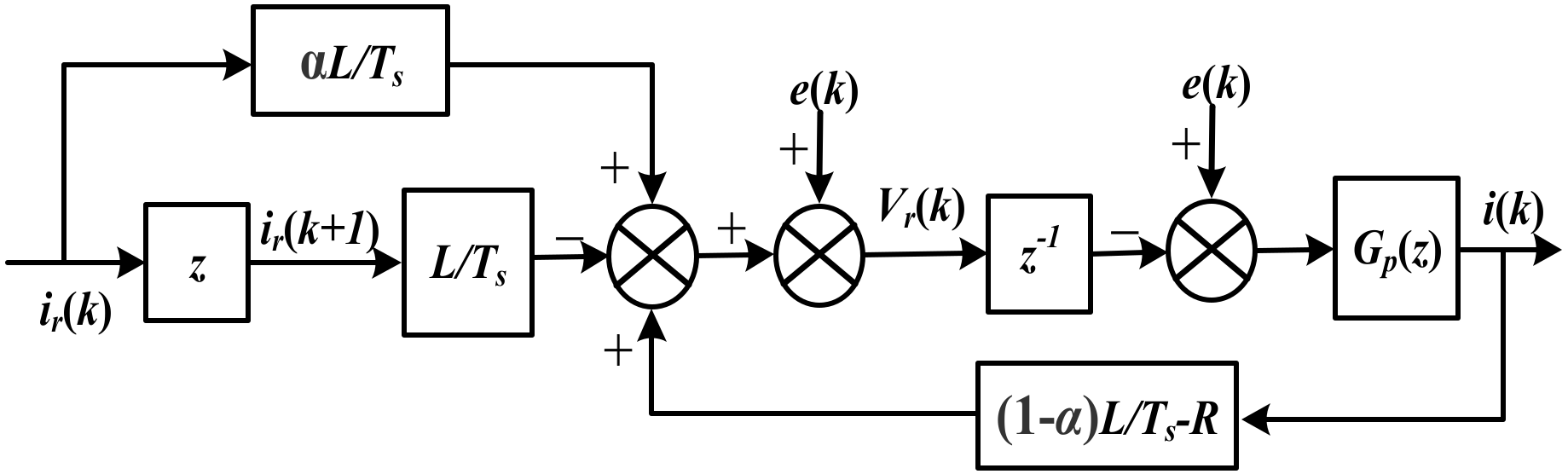
3.2.1. The Improved DBC with Error Correction

In [33,34], it was claimed that deadbeat control can promise zero-tracking error in the next sampling interval, which means:

$$i_r\left(k+1\right)-i\left(k+1\right)=0$$

(10)

Hence, the prediction model of the traditional DBC can be given as:

$$V_r\left(k\right)=e\left(k\right)+\left(\frac{L}{T_s}-R\right)i\left(k\right)-\frac{L}{T_s}{i}_r\left(k+1\right)$$

(11)

where V_r(k) is the predicted reference value of the rectifier voltage at the kth instant.

Once model mismatch occurred, V_r(k) differed from the original value, which influenced the performance of the system and could even cause system instability. Thus, an error correction term was introduced in order to compensate for the current error. The modified prediction model of the improved DBC can be depicted as:

$$V_r\left(k\right)=e\left(k\right)+\left(\frac{L}{T_s}-R\right)i\left(k\right)-\frac{L}{T_s}{i}_r\left(k+1\right)-\alpha \frac{L}{T_s}\left[i\left(k\right)-i_r\left(k\right)\right]$$

(12)

where α is the control coefficient.

3.2.2. The Improved FCS–MPC with Error Correction

Because of the computational burden of the conventional FCS–MPC, the simplified FCS–MPC was proposed in [35], the predicted model of which could also be described as Equation (11). Hence, according to Equations (11) and (12), the improved FCS–MPC with error correction can be calculated as follows:

$$V_r\left(k\right)=e\left(k\right)+\left(\frac{L}{T_s}-R\right)i\left(k\right)-\frac{L}{T_s}{i}_r\left(k+1\right)-\gamma \frac{L}{T_s}\left[i\left(k\right)-i_r\left(k\right)\right]$$

(13)

where γ is control coefficient of the improved FCS–MPC.

The switching states of S_a and S_b are defined as follows:

$$S_a=\left\{\begin{array}{c}1{\mathit{if}\mathit{S}}_1{\mathit{is}\mathit{on}\mathit{and}\mathit{S}}_2\mathit{is}\mathit{off}\\ 0{\mathit{if}\mathit{S}}_1{\mathit{is}\mathit{off}\mathit{and}\mathit{S}}_2\mathit{is}\mathit{on}\end{array}\right.$$

(14)

$$S_b=\left\{\begin{array}{c}1{\mathit{if}\mathit{S}}_3{\mathit{is}\mathit{on}\mathit{and}\mathit{S}}_4\mathit{is}\mathit{off}\\ 0{\mathit{if}\mathit{S}}_3{\mathit{is}\mathit{off}\mathit{and}\mathit{S}}_4\mathit{is}\mathit{on}\end{array}\right.$$

(15)

Thus, according to the working principle of the rectifier and the traits of the insulated gate bipolar transistor (IGBT) [32], V(k) can be calculated as:

$$V\left(k\right)=V_{dc}\left(S_a-S_b\right)$$

(16)

where V_dc is the DC voltage of the rectifier, and S_a, S_b are the switching state of the bridge legs.

Finally, the cost function of the improved FCS-MPC is chosen as:

$$J=\left|V_r\left(k\right)-V\left(k\right)\right|.$$

(17)

4. Impact of the Control Coefficient and Selection of the Switching Condition

The above section demonstrated the proposed control, consisting of improved DBC and MPC. In this section, the impact of the control coefficient to system performance was analyzed and a switching condition was proposed. According to Equation (9), α and γ can be limited as:

$$-1<\alpha <1$$

(18)

$$-1<\gamma <1$$

(19)

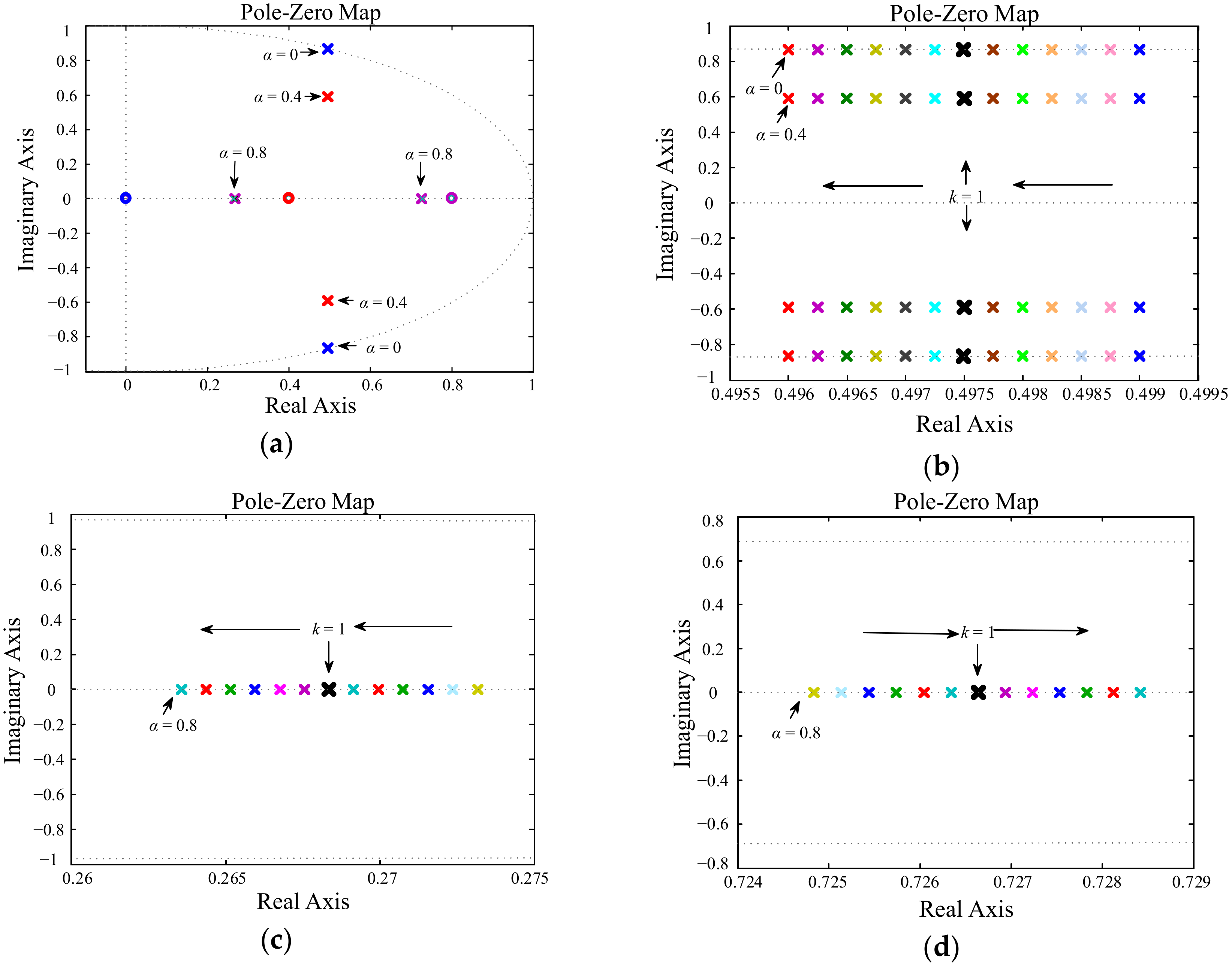
4.1. Robustness Analysis of α for the Improved DBC

According to the previous work [28], delay exits were present in every digital system, and it was assumed as long as a control period.

A discrete control block diagram of the improved DBC is given in Figure 3.

The transfer function of the inductor in S domain could be written as:

$$G_p\left(s\right)=\frac{1}{sL+R}$$

(20)

Including the delay of a control period by z⁻¹ block, G_p(s) could be rewritten in Z domain as:

$$G_p\left(z\right)=\left(1-z^{-1}\right)Z\left[\frac{G_p\left(s\right)}{s}\right]=\frac{T_s}{L}\frac{1}{z-\left(1-R{T}_s/L\right)}$$

(21)

The closed-loop transfer function using e(k) as the disturbance is expressed as follows:

$$G\left(z\right)=\frac{i\left(k\right)}{i_r\left(k\right)}=\frac{\left(k_{3}z-k_1\right)z^{-1}{G}_p\left(z\right)}{1+k_2{z}^{-1}{G}_p\left(z\right)}=\frac{z-\alpha }{z^2-\left(1-R\frac{T_s}{L}\right)z+\left(1-\alpha -R\frac{T_s}{L}\right)}$$

(22)

where k₁ = αL/T_s, k₂ = (1−α)L/T_s−R, and k₃ = L/T_s.

To promise the system is stable, the following items should be met:

$$0<1-\alpha -R{T}_s/L<1$$

(23)

According to the actual experimental parameters, L, R, and T_s are 3.1 mH, 0.3 Ω, and 100 us, respectively. Moreover, based on Equations (20) and (25), the constraint of the control coefficient α is shown as follows:

$$-0.005<\alpha <0.995$$

(24)

In order to study the influence of the changes on inductor parameter, the pole locus was analyzed based on the different values of α [28].

The closed-loop transfer function G(z)_a could be modified by replacing L with the actual value of L_a, given as follows:

$$G{(z)}_a=\frac{i\left(k\right)}{i_r\left(k\right)}=\frac{\left(k_{3a}z-k_{1a}\right)z^{-1}{G}_p{(z)}_a}{1+k_{2a}{z}^{-1}{G}_p{(z)}_a}=\frac{z-\alpha }{z^2-\left(1-R\frac{k{T}_s}{L}\right)z+\left(1-\alpha -R\frac{k{T}_s}{L}\right)}$$

(25)

where k_1a = αL_a/T_s, k_2a = (1−α)L_a/T−R, k_3a = L_a/T, and k = L/L_a.

In Figure 4, in which the zero-pole diagrams of different k with different α are presented, it can be seen that the larger the α, the farther the poles are from the unit circle, resulting in the stronger robustness.

4.2. Robustness Analysis of γ for the Improved FCS–MPC

Similar to the last section, the impact of γ for the improved FCS–MPC was analyzed in this section.

The error between V_r(k) and V(k) is taken as:

$$\mathsf{\Delta }v\left(k\right)=V_r\left(k\right)-V\left(k\right)$$

(26)

Figure 5 denotes that when the reference value is calculated as V_r1(k), V₁(k) should be chosen. Similarly, V₂(k) should be chosen corresponding to V_r2(k). Thus, the error between V_r(k) and V(k) is bounded:

$$\Vert \mathsf{\Delta }v\left(k+1\right)\Vert \le 0.5V_{dc}$$

(27)

The following stability criteria for the Lyapunov function G(Δy(k)) are described in [29,35]:

$$\begin{gathered} G\left(\mathsf{\Delta }i\left(k\right)\right)\ge c_1{\left|\mathsf{\Delta }i\left(k\right)\right|}^l, \forall \mathsf{\Delta }i\left(k\right)\in H \\ G\left(\mathsf{\Delta }i\left(k\right)\right)\le c_2{\left|\mathsf{\Delta }i\left(k\right)\right|}^l, \forall \mathsf{\Delta }i\left(k\right)\in \Gamma \\ G\left(\mathsf{\Delta }i\left(k+1\right)\right)-G\left(\mathsf{\Delta }i\left(k\right)\right)<-c_3{\left|\mathsf{\Delta }i\left(k\right)\right|}^l+c_4 \end{gathered}$$

(28)

where c₁, c₂, c₃, and c₄ are positive constants, and l ≥ 1 is a positive control invariant set and compact set.

According to [29], the Lyapunov function rate of change, ΔG (Δi(k)), could be depicted as follows:

$$\mathsf{\Delta }G\left(\mathsf{\Delta }i\left(k\right)\right)=\frac{1}{2}\left({\gamma }^2-1\right)\mathsf{\Delta }{i}^2\left(k\right)+\frac{1}{2}{\left[\frac{T_s}{L}\mathsf{\Delta }v\left(k+1\right)\right]}^2-\gamma \frac{T_s}{L}\mathsf{\Delta }v\left(k+1\right)\mathsf{\Delta }i\left(k\right)$$

(29)

Solving Equation (29), it could be rewritten as:

$$\begin{gathered} \mathsf{\Delta }G\left(\mathsf{\Delta }i\left(k\right)\right)=\left(\frac{1}{2}-b\right)\left({\gamma }^2-1\right)\mathsf{\Delta }{i}^2(k+p\left(\mathsf{\Delta }i\left(k\right)\right), \\ p\left(\Delta i\left(k\right)\right)=b\left({\gamma }^2-1\right)\Delta i^2\left(k\right)-\gamma \frac{T_s}{L}\Delta v\left(k+1\right)\Delta i\left(k\right)+\frac{1}{2}{\left[\frac{T_s}{L}\Delta v\left(k+1\right)\right]}^2 \end{gathered}$$

(30)

where b is a positive constant from 0 to 1/2.

Therefore, the maximum of p(Δi(k)) is given as Equation (31):

$$p(\mathsf{\Delta }i\left(k\right){)}_{max}{\left[\frac{T}{L_s}\mathsf{\Delta }v\left(k+1\right)\right]}^2\frac{\left(1-2b\right){\gamma }^2+2b}{4b\left(1-{\gamma }^2\right)}.$$

(31)

Based on Equations (29)–(31), ΔG (Δi(k)) could be expressed as:

$$\mathsf{\Delta }G\left(\mathsf{\Delta }i\left(k\right)\right) \le \left(\frac{1}{2}-b\right)\left({\gamma }^2-1\right)\mathsf{\Delta }{i}^2\left(k\right)+p(\mathsf{\Delta }i\left(k\right){)}_{max}\le \left(\frac{1}{2}-b\right)\left({\gamma }^2-1\right)\mathsf{\Delta }{i}^2\left(k\right)+\frac{1}{4}\left(\frac{T_s}{L}{V}_{dc}\right){}^2\frac{\left(1-2b\right){\gamma }^2+2b}{4b\left(1-{\gamma }^2\right)}.$$

(32)

Thus, according to Equations (28) and (32), the following equation is defined:

$$\begin{gathered} c_1=c_2=1; \\ {c}_3=\left(\frac{1}{2}-b\right)\left(1-{\gamma }^2\right); \\ {c}_4=\frac{1}{4}{(\frac{T_s}{L}{V}_{dc})}^2\frac{\left(1-2b\right){\gamma }^2+2b}{4b\left(1-{\gamma }^2\right)} \end{gathered}$$

(33)

The rate of the change of the Lyapunov function is considered as:

$$\mathsf{\Delta }G\left(\mathsf{\Delta }i\left(k\right)\right)\le -2c_{3}G\left(\mathsf{\Delta }i\left(k\right)\right)+c_4$$

(34)

This means that the current error converges to the compact set as:

$$A=\left\{\mathsf{\Delta }i\left(k\right)|||\mathsf{\Delta }i\left(k\right)||\le \sqrt{\frac{c_4}{c_3}}=\sqrt{\frac{\frac{1}{4}{(\frac{T_s}{L}{V}_{dc})}^2\frac{\left(1-2b\right){\gamma }^2+2b}{4b}}{\frac{1}{2}b}}\right\}$$

(35)

Equation (35) implies that when γ becomes larger, the current error is smaller. Namely, the robustness is stronger as γ grows larger.

4.3. Transient Response of the Control Coefficient

Based on Equation (8), G (Δi(k)) could be calculated as:

$$G\left(\mathsf{\Delta }i\left(k+1\right)\right)=\frac{1}{2}{d}^{2}G\left(\mathsf{\Delta }i\left(k\right)\right)$$

(36)

Hence, the convergence rate of the Lyapunov function could be investigated by ρ, which is defined as:

$$\rho =\frac{G\left(\mathsf{\Delta }i\left(k\right)\right)}{G\left(\mathsf{\Delta }i\left(k+1\right)\right)}=\frac{1}{d^2}$$

(37)

As described in [36], ρ is proportional to the dynamic response, which means the system becomes faster as ρ increases. As depicted in Figure 6, as d becomes larger, ρ becomes smaller; namely, the transient time becomes longer as the robustness improves. As a result, we should select the control coefficients in compromise to take into account the robustness and convergence speed of the system simultaneously.

Therefore, based on the previous analysis, α and γ were set to 0.5 and 0.4, respectively.

4.4. Analysis of the Swithing Condition

When error correction is implemented, based on the Lyapunov theorem, the current error gradually converges to 0, and its rate should be less than 1. When the reference current changes, it would satisfy the following inequation:

$$\left|\frac{\mathsf{\Delta }i\left(k\right)}{\mathsf{\Delta }i\left(k-1\right)}\right|>1$$

(38)

Thus, we define the switching condition as:

$$G=\left|\frac{\mathsf{\Delta }i\left(k\right)}{\mathsf{\Delta }i\left(k-1\right)}\right|=\left|\frac{i_r\left(k\right)-i\left(k\right)}{i_r\left(k-1\right)-i\left(k-1\right)}\right|$$

(39)

and:

$$G_{th}=1$$

(40)

where G_th is the threshold value.

If G is larger than G_th, the reference current changes, so the improved FCS–MPC was used to achieve a fast transient performance. If G is smaller than or equal to G_th, the converter system is stable, so the improved DBC was used to achieve a better performance with a constant switching frequency.

5. Experimental Results

A single-phase rectifier prototype was adopted to validate the presented hybrid control method, as shown in Figure 7. The specific experimental parameters are presented in

Table 1. Experimental parameters.

Symbol	System Parameters	Value
e	grid voltage	50 V/50 Hz
L	Filter inductance	3.1 mH
R	Equivalent series resistance	0.3 Ω
C	DC side capacitor	1000 μF
Ts	Sampling period	100 us

. A digital signal processing (DSP) system consisting of a TMS320F28069 (Texas Instruments, Dallas, TX, USA) was utilized to carry out the proposed control strategy. A Tektronix oscilloscope was used to obtain the current waveforms and a power analyzer was utilized to analyze these waveforms. For easier verification, different grid current references were given directly.

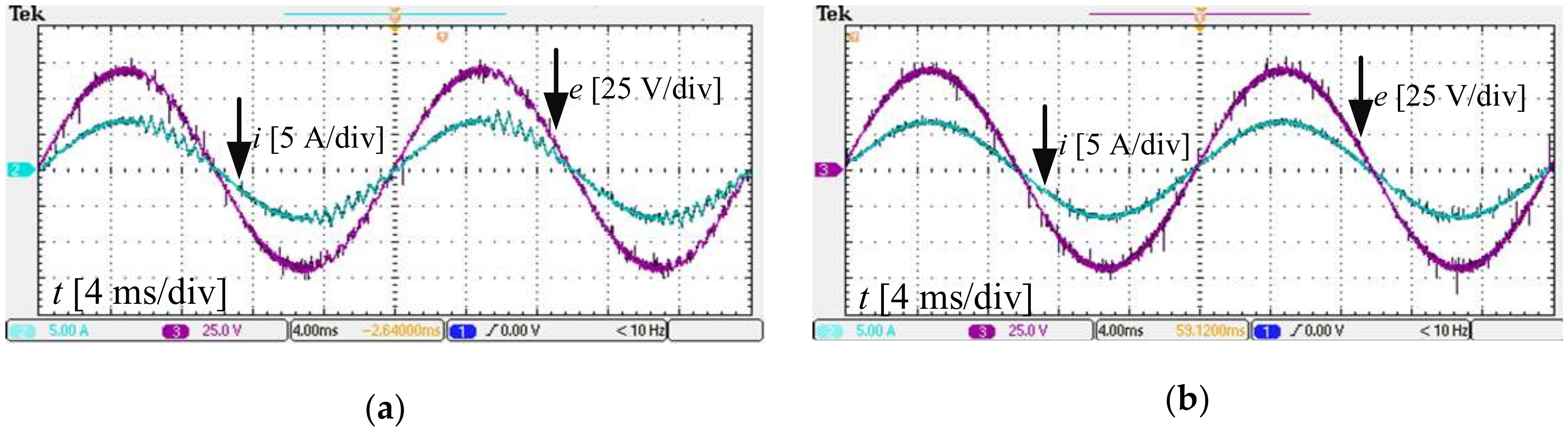
5.1. Steady-State Performance

When the converter was in the steady state, the improved DBC was used to maintain better steady-state performance. The experimental results for steady state between the conventional FCS–MPC and the proposed control strategy are shown in Figure 8. It was observed that with the implementation of the proposed control strategy, the THD of the grid current was 1.86%, while that of the conventional FCS–MPC was 4.62%. Moreover, the harmonic frequency was focused on switching frequency 10 kHz using the proposal. By contrast, the current harmonics were spread with the conventional control. As the harmonic spectrum of the input current represented the distribution of the switching frequency in single-phase rectifiers, it proved that the proposed control achieves fixed switching frequency.

The results above convincingly present that the proposal had more amendatory performance than the conventional FCS–MPC in steady condition, and that it not only achieved constant switching frequency but also lowered the THD of the grid current.

5.2. Dynamic Response Performance

To validate the excellent transient response of the presented control compared to the conventional FCS–MPC, two reference current step changes (from 4 to 6.8 A, and 6.8 to 4 A, respectively) were generated in both the proposed control strategy and the conventional FCS–MPC.

In Figure 9a, it takes 238 μs to reach a steady-state level with a reference current step up, while it takes 256 μs in Figure 9b. The settling time in Figure 10a,b is 379 and 388 μs, respectively. These results illuminate that the dynamic response of the two control methods is nearly the same.

5.3. Investigation of Robustness

Model mismatch existed in almost all of the predictive controls, restricting the performance of the converter, and even deteriorating stability. The experimental results of the current behavior of different values of inductance are demonstrated in Figure 11 and Figure 12. It was seen that when the variation of the inductor valued in the range of −20% to +20%, oscillation of the current both appeared in the conventional FCS–MPC. However, stronger robustness was obtained with the utilization of the proposal.

6. Conclusions

In this paper, a hybrid control strategy with error correction for fixed frequency and stronger robustness, based on improved DBC and FCS–MPC, was presented.

To realize a generated frequency spectrum, the proposed control strategy used a switched way, in which the system adopted the improved DBC in the steady state, and the improved FCS–MPC was utilized in the transient stage. For the model mismatch problems, both DBC and FCS–MPC were modified with error correction to compensate for the current error. More importantly, the error correction term was combined with the Lyapunov method so that the current error converged to zero with improved robustness. Finally, the proposed method calculated the control coefficient and defined the switching condition with the Lyapunov stability theorem.

To demonstrate the effectiveness and practicability of the proposal, a single-phase voltage source rectifier prototype was set up. The results validate the merits mentioned above, including fixed switching frequency, lower THD, and stronger robustness. This kind of control strategy plays a promising role in the development of predictive control.

References

1. Testud, J.L.; Richalet, J.; Rault, A.; Papon, J. Model predictive heuristic control: Application to industrial processes. Automatica 1978, 14, 413–428. [Google Scholar]
2. Car, G.K.; Skrjanc, I. Tracking-error model-based predictive control for mobile robots in real time. J. Robot. Auton. Syst. 2007, 55, 460–469. [Google Scholar]
3. Rodriguez, J.; Cortes, P. Predictive Control of Power Converters and Electrical Drives; John Wiley & Sons Ltd.: Hoboken, NJ, USA, 2012. [Google Scholar]
4. Morari, M.; Lee, J.H. Model predictive control: Past, present and future. Comput. Chem. Eng. 1999, 23, 667–682. [Google Scholar] [CrossRef]
5. Camacho, E.F.; Bordons, C. Model predictive control. In Advanced Textbooks in Control and Signal Processing; Springer: London, UK, 2004. [Google Scholar]
6. Aguirre, M.; Kouro, S.; Rojas, C.A.; Rodriguez, J.; Leon, J.I. Switching Frequency Regulation for FCS-MPC Based on a Period Control Approach. IEEE Trans. Ind. Electron. 2018, 65, 5764–5773. [Google Scholar] [CrossRef]
7. Mariethoz, S.; Beccuti, A.G.; Papafotiou, G.; Morari, M. Sensorless explicit model predictive control of the DC-DC buck converter with inductor current limitation. In Proceedings of the Twenty-Third Annual IEEE Applied Power Electronics Conference and Exposition, Austin, TX, USA, 24–28 February 2008. [Google Scholar]
8. Preindl, M.; Schaltz, E. Sensorless model predictive direct current control using novel second order PLL-observer for PMSM drive systems. IEEE Trans. Ind. Electron. 2011, 58, 4087–4095. [Google Scholar] [CrossRef]
9. Rodriguez, J.O.S.E.; Pontt, J.O.R.G.E.; Silva, C.E.S.A.R.; Salgado, M.; Rees, S.; Ammann, U.; Cortés, P. Predictive control of three-phase inverter. Electron. Lett. 2004, 40, 561–562. [Google Scholar] [CrossRef]
10. Rodriguez, J.; Pontt, J.; Silva, C.A.; Correa, P.; Lezana, P.; Cortés, P.; Ammann, U. Predictive current control of a voltage source inverter. IEEE Trans. Ind. Electron. 2007, 54, 495–503. [Google Scholar] [CrossRef]
11. Salinas, F.; Gonzalez, M.A.; Escalante, M.F. Finite control set model predictive control of a flying capacitor multilevel chopper using petri nets. IEEE Trans. Ind. Electron. 2016. [Google Scholar] [CrossRef]
12. Vazquez, S.; Leon, J.I.; Franquelo, L.G.; Rodriguez, J.; Young, H.A.; Marquez, A.; Zanchetta, P. Model predictive control: A review of its applications in power electronics. IEEE Ind. Electron. Mag. 2014, 8, 16–31. [Google Scholar] [CrossRef]
13. Zhang, Y.; Xie, W.; Li, Z.; Zhang, Y. Low Complexity Model Predictive Power Control—Double Vector-Based Approach. IEEE Trans. Power Electron. 2014, 61, 5871–5880. [Google Scholar] [CrossRef]
14. Zhang, Y.; Xie, W.; Li, Z.; Zhang, Y. Model predictive direct power control of PWM rectifier with duty cycle optimization. IEEE Trans. Power Electron. 2013, 28, 5343–5351. [Google Scholar] [CrossRef]
15. Zhang, Y.; Liu, J.; Yang, H.; Fan, S. New Insights into Model Predictive Control for Three-Phase Power Converters. IEEE Trans. Ind. Appl. 2019, 55, 1973–1982. [Google Scholar] [CrossRef]
16. Hu, J. Improved dead-beat predictive DPC strategy of grid-connected DC-AC converters with switching loss minimization and delay compensations. IEEE Trans. Ind. Inform. 2013, 9, 728–738. [Google Scholar] [CrossRef]
17. Hu, J.; Zhu, Z.Q. Improved voltage-vector sequences on dead-beat predictive direct power control reversible three-phase grid-connected voltage-source converters. IEEE Trans. Power Electron. 2008, 28, 254–267. [Google Scholar] [CrossRef]
18. Cortés, P.; Rodríguez, J.; Quevedo, D.E.; Silva, C. Predictive current control strategy with imposed load current spectrum. IEEE Trans. Power Electron. 2008, 23, 612–618. [Google Scholar] [CrossRef]
19. Tarisciotti, L.; Formentini, A.; Gaeta, A.; Degano, M.; Zanchetta, P.; Rabbeni, R.; Pucci, M. Model Predictive Control for Shunt Active Filters with Fixed Switching Frequency. IEEE Trans. Ind. Appl. 2017, 53, 296–304. [Google Scholar] [CrossRef]
20. Young, H.A.; Perez, M.A.; Rodriguez, J. Analysis of finite control set model predictive current control with model parameter mismatch in a three phase inverter. IEEE Trans. Ind. Electron. 2016, 63, 3100–3107. [Google Scholar] [CrossRef]
21. Xia, C.; Wang, M.; Song, Z.; Liu, T. Robust model predictive current control of three-phase voltage source PWM rectifier with online disturbance observation. IEEE Trans. Ind. Inform. 2012, 8, 459–471. [Google Scholar] [CrossRef]
22. Du, G.; Li, J.; Liu, Z. The improved model predictive control based on novel error correction between reference and predicted current. In Proceedings of the 2018 IEEE Applied Power Electronics Conference and Exposition (APEC), San Antonio, TX, USA, 4–8 March 2018; pp. 3005–3010. [Google Scholar]
23. Li, H.; Liu, S. Speed control for PMSM servo system using predictive functional control and extended state observer. IEEE Trans. Ind. Electron. 2012, 59, 1171–1183. [Google Scholar] [CrossRef]
24. Espí, J.M.; Castello, J.; García-Gil, R.; Garcera, G.; Figueres, E. An adaptive robust predictive current control for three-phase grid-connected inverters. IEEE Trans. Ind. Electron. 2011, 58, 3537–3546. [Google Scholar] [CrossRef] [Green Version]
25. Arif, B.; Tarisciotti, L.; Zanchetta, P.; Clare, C.J.; Degano, M. Grid Parameter Estimation Using Model Predictive Direct Power Control. IEEE Trans. Ind. Appl. 2015, 51, 4614–4622. [Google Scholar] [CrossRef] [Green Version]
26. Shen, K.; Zhang, J. Modeling Error Compensation in FCS-MPC of a Three-phase Inverter. In Proceedings of the IEEE International Conference on Power Electronics, Drives and Energy Systems, Bengaluru, India, 16–19 December 2012; pp. 1–6. [Google Scholar]
27. Siami, M.; Khaburi, D.A.; Abbaszadeh, A.; Rodríguez, J. Robustness Improvement of Predictive Current Control Using Prediction Error Correction for Permanent-Magnet Synchronous Machines. IEEE Trans. Ind. Electron. 2016, 63, 3458–3466. [Google Scholar] [CrossRef]
28. Du, G.; Li, J.; Du, F.; Liu, Z. A Robust Digital Control Strategy Using Error Correction Based on the Discrete Lyapunov Theorem. Energies 2018, 11, 848. [Google Scholar]
29. Du, G.; Liu, Z.; Du, F.; Li, J. Performance Improvement of Model Predictive Control Using Control Error Compensation for Power Electronic Converters Based on the Lyapunov Function. J. Power Electron. 2017, 17, 983–990. [Google Scholar]
30. Kwak, S.; Yoo, S.J.; Park, J. Finite control set predictive control based on Lyapunov function for three-phase voltage source inverters. IET Power Electron. 2014, 7, 2726–2732. [Google Scholar] [CrossRef]
31. Parvez, M.; Mekhilef, S.; Tan, N.M.L.; Akagi, H. A robust modified model predictive control (MMPC) based on Lyapunov function for three-phase active-front-end (AFE) rectifier. In Proceedings of the 2016 IEEE Applied Power Electronics Conference and Exposition (APEC), Long Beach, CA, USA, 18–24 March 2016; pp. 1163–1168. [Google Scholar]
32. Akter, M.P.; Mekhilef, S.; Tan, N.M.L.; Akagi, H. Modified model predictive control of a bidirectional AC-DC converter based on Lyapunov function for energy storage systems. IEEE Trans. Ind. Electron. 2016, 63, 704–715. [Google Scholar] [CrossRef]
33. Young, H.A.; Perez, M.A.; Rodriguez, J.; Abu-Rub, H. Assessing Finite-Control-Set Model Predictive Control: A Comparison with a Linear Current Controller in Two-Level Voltage Source Inverters. IEEE Ind. Electron. Mag. 2014, 8, 44–52. [Google Scholar] [CrossRef]
34. Xie, W.; Wang, X.; Wang, F.; Xu, W.; Kennel, R.M.; Gerling, D.; Lorenz, R.D. Finite-Control-Set Model Predictive Torque Control with a Deadbeat Solution for PMSM Drives. IEEE Trans. Ind. Electron. 2015, 62, 5402–5410. [Google Scholar] [CrossRef]
35. Abbaszadeh, A.; Khaburi, D.A.; Mahmoudi, H.; Rodríguez, J. Simplified model predictive control with variable weighting factor for current ripple reduction. IET Power Electron. 2017, 10, 1165–1174. [Google Scholar] [CrossRef]
36. Slotineand, J.-J.E.; Li, W. Applied Nonlinear Control, Englewood Cliffs; Prentice-Hall: Upper Saddle River, NJ, USA, 1991. [Google Scholar]
Figure 1. Single phase rectifier topology.
Energies 13 01176 g001
Figure 2. Flowchart of the proposed control method.
Energies 13 01176 g002
Figure 3. Control block diagram of the current loop.
Energies 13 01176 g003
Figure 4. Pole locus diagrams of G(z)a with changes of k (from 0.4 to 1.6 with increments of 0.1) based on different values of α: (a) the whole sight of pole locus; (b) the pole locus based on α = 0 and α = 0.4; (c) the pole locus based on α = 0.8; (d) the pole locus based on α = 0.8.
Energies 13 01176 g004
Figure 5. The error between Vr(k) and V(k).
Energies 13 01176 g005
Figure 6. The relationship between ρ and d.
Energies 13 01176 g006
Figure 7. The experimental prototype.
Energies 13 01176 g007
Figure 8. Experimental results of the grid current for steady state: (a) the harmonic spectrum of the conventional finite control set model predictive control (FCS–MPC); (b) the harmonic spectrum of the proposed control strategy.
Energies 13 01176 g008
Figure 9. Experimental results of current behavior during a reference current step up from 4 to 6.8 A peak: (a) the conventional FCS–MPC; (b) the proposed control strategy.
Energies 13 01176 g009
Figure 10. Experimental results of current behavior during a reference current step down from 6.8 to 4 A peak: (a) the conventional FCS-MPC; (b) the proposed control strategy.
Energies 13 01176 g010
Figure 11. Experimental results of current behavior when the inductance deviation is −20%: (a) the conventional FCS–MPC; (b) the proposed control strategy.
Energies 13 01176 g011
Figure 12. Experimental results of current behavior when the inductance deviation is +20%: (a) the conventional FCS–MPC; (b) the proposed control strategy.
Energies 13 01176 g012