Analysis of the Thermodynamic Consistency of the Richardson–Duhmann Model for Thermionic Converters

Abstract

In this work, we develop the general theory for analyzing the thermodynamic consistency of the Richardson–Duhmann model for vacuum thermionic energy converters. In addition to the electron fluxes from emitter to collector and vice versa, we calculate the energy and entropy fluxes associated to them. The calculation of the entropy fluxes is what allows us to conclude that the model is consistent by verifying that both at the emitter and at the collector the entropy generation rate is positive. In the process, we review the Richardson–Duhmann model in order to assure that the assumptions we make for calculating the energy and entropy fluxes are consistent. We also generalize the Richardson–Duhmann model in order to consider Fermi–Dirac statistics.

1. Introduction

Vacuum thermionic energy converters (VTEC) are an option for converting heat into electricity that relies on the flow of electrons through vacuum gaps. From the theoretical point of view, they are a highly efficient alternative to thermo-electrics [1], as well as a key part of several novel concepts such as photon-enhanced thermionic emission (PETE) [2] and hybrid thermionic-photovoltaic energy conversion [3]. The basic model for calculating the ideal current–voltage characteristic of a thermionic converter is the Richardson–Duhmann model [4] that allows the electron fluxes between emitter (cathode) and collector (anode) to be calculated from which the efficiency of the converter can be derived. However, several assumptions are involved in this model and we wonder if these assumptions led, at the end, to a model consistent with the laws of thermodynamics. To verify this consistency, we have developed next a thermodynamic model that allows the entropy generation rate at the emitter and at the collector to be calculated in order to check these are positive or zero. To develop this model, we first review the working hypothesis of the Richardson–Duhmann model so that we make sure we use the same hypothese when calculating the entropy fluxes. Hypothese related to the electron density of states and electron velocity distribution are reviewed in Section 2 by considering the thermionic emitter in equilibrium. Then, we also include the presence of the collector in equilibrium (Section 3), which will allow us to formulate the energy and entropy fluxes between both and, in Section 4 we generalize the analysis for operating conditions out of the equilibrium, that is, with the emitter hot and the collector biased. Finally, in Section 5, we analyze the thermodynamic consistency of the model.

2. Thermionic Emitter in Equilibrium

Figure 1 represents the distribution of electrostatic potential energy ($-e\varphi$) in equilibrium, from the bulk to its surface, of which will later become a thermionic emitter. The Richardson–Duhmann equation models the current-density, J_E, of electrons emitted as a function of the temperature, $T_E$, of this emitter as follows:

$$J_E(T_E)=-e{\dot{N}}_{EC}=-A{T}_E^2\exp \frac{-{\mathsf{\Phi }}_E}{k_B{T}_E}$$

(1)

where e is the charge of the electron (in absolute value), ${\dot{N}}_{EC}$ is the number of electrons emitted per unit of time and area by the emitter (this apparently strange notation is used in order to preserve self-consistency with the discussions that will follow), A is the Richardson constant, Φ_E is the emitter work-function, and k_B is the Boltzmann constant. The minus sign only accounts for the fact that, if electrons flow from left to right, then the electron current density goes from right to left. The Richardson constant is given by:

$$A=\frac{4e{k}_B^2{m}_e\pi }{h^3}=1.20\times {10}^6 {\mathrm{Am}}^{-2}{\mathrm{K}}^2$$

(2)

where $m_e$ is the mass of the electron at rest and h is the Planck constant.

In order to clarify the discussions that follow in this paper, it is convenient to quickly review the derivation of Equation (2), as well as the hypothese involved in this derivation.

First, the work-function Φ_E is defined as the minimum energy that is demanded in order to make an electron escape from the emitter. This level is referred to the Fermi level in the idea that the Fermi level indicates the last energy level occupied by an electron in the emitter. However, this is only strictly true at 0 K and, approximately true, at higher temperatures, when the density of electronic states in the emitter is very high (as it is assumed to be the case of metals). Notice (Figure 1) that the work-function Φ_E is also the maximum of the electrostatic potential energy distribution across the interface of the thermionic emitter. Φ_E can be affected in practical cases by the presence of image charges. In spite of these facts, we will assume that the work-function is a property of the emitter material that does not depend on the temperature nor is impacted by charge images. This is a common assumption and will not alter the concepts in this work.

Secondly, once the electron has left the emitter and the interface where there is some charge density, we will assume it becomes a free electron. Under this assumption, its kinetic energy, ${ϵ}_{kt}$, just when the electron has left the emitter and become free, is given by:

$${ϵ}_{kt}(k)=ϵ-{\mathsf{\Phi }}_E=\frac{1}{2}{m}_e{v}^2=\frac{1}{2}\frac{{\hslash }^2{k}^2}{m_e}$$

(3)

where ϵ is the total energy of the electron, $v$ is the speed of the electron, and k is the modulus of the electron wave-vector. We are reminded here that, since the Fermi level has been taken as our zero energy reference, Φ_E corresponds also to the electrostatic potential energy of the electron at the point where the electron has become free.

The density of states available to electrons with wave-vector of between k and dk, $\widehat{g}(\mathit{k})d^3\mathit{k}$, is given by:

$$\widehat{g}(\mathit{k})d^3\mathit{k}=\frac{2}{{(2\pi )}^3}{d}^3\mathit{k}=\frac{2}{{(2\pi )}^3}4\pi k^{2}dk=g(k)dk$$

(4)

where factor 2 at the numerator comes from considering electron spin degeneracy. Spherical coordinates have been used for expressing the differential volume d³k as $4\pi k^{2}dk$. Using Equation (3) for substituting k as a function of the electron total energy ϵ, the density of states in Equation (4) can be expressed also as:

$$g(k)dk=g(ϵ)dϵ=\{\begin{array}{c}\frac{4{(2m_e)}^{\frac{3}{2}}\pi {(ϵ-{\mathsf{\Phi }}_E)}^{1/2}}{h^3}\\ 0ϵ<{\mathsf{\Phi }}_E\end{array}ϵ\ge {\mathsf{\Phi }}_E$$

(5)

In Equation (5), we have assumed that no electron tunneling takes place (and therefore, that there are no electron states for $ϵ<{\mathsf{\Phi }}_E$) so that only electrons with energy above Φ_E can leave the emitter. The electron current density, $J_E$, due to the flux of electrons leaving the emitter is given by:

$$J_E(T_E,E_F)=-e{\displaystyle \underset{{\Phi }_{E,0,0}}{\overset{\infty ,\pi /2,\pi /2}{\iiint }}}g(ϵ)f(ϵ,E_F,T_E)\frac{v(ϵ-{\Phi }_E)}{4\pi }sin\theta cos\theta d\phi d\theta dϵ$$

(6)

where,

$$f(ϵ,E_F,T_E)=\frac{1}{\exp \frac{ϵ-E_F}{k_B{T}_E}+1}$$

(7)

is the Fermi–Dirac distribution function,

$$v(ϵ-{\mathsf{\Phi }}_E)={\left[\frac{2(ϵ-{\mathsf{\Phi }}_E)}{m_e}\right]}^{1/2},$$

(8)

Obtained from Equation (3), is the modulus of the velocity of a free electron with energy ϵ. The factor 4π in the denominator comes from assuming that the electron velocity is equally distributed in all directions, θ is the angle of incidence of the vector velocity with the cathode surface (Figure 2) and $d\mathsf{\Omega }=\sin \theta \mathrm{d}\theta \mathrm{d}\mathsf{\phi }$ is the differential of the solid angle.

If we assume the electron gas is nondegenerated, then,

$$f(ϵ,E_F,T_E)\approx \exp \frac{-ϵ+E_F}{k_B{T}_E}$$

(9)

and Equation (5) leads finally to:

$$J_E(T_E)\approx -A{T}_E^2\exp \frac{-{\mathsf{\Phi }}_E}{k_B{T}_E}\exp \frac{-E_F}{k_B{T}_E}$$

(10)

Which is the equation we wanted to demonstrate taking into account that we have taken as zero the energy reference level $E_F=0$.

Equation (5) still needs to be corrected for equilibrium conditions since in equilibrium, whatever the temperature $T_E$ is, the emitter cannot emit any net electron flux. The common assumption is that, in equilibrium, achieved at room temperature, $T_E=T_C$, the electron flux emitted from the emitter is exactly balanced by an electron flux that we will designate for convenience as ${\dot{N}}_{EC,0}$, coming from the electron cloud that builds-up in the vicinity of the emitter as more and more electrons leave the emitter. This electron cloud is actually the negative charge density that appears close to the emitter surface and that has also been represented in Figure 1c. Consequently,

$${\dot{N}}_{EC,0}=-J_E(T_C)/e\approx \frac{1}{e}A{T}_C^2\exp \frac{-{\mathsf{\Phi }}_E}{k_B{T}_C}$$

(11)

It is conceptually important to realize that, in equilibrium, once we move away from this electron cloud, the electric field is zero and, therefore, the electrostatic potential has to be constant, as it also has been represented in Figure 1. The consequence of this is that, the density of states calculated in Equation (5) for a point right outside the emitter (once it has left the electron cloud close to the emitter), is also valid far away from the emitter because electrons are also still free far away from the emitter. Although this assessment might look obvious at this stage, it will not be that obvious when the emitter is placed in front of a collector.

3. Thermionic Emitter in the Presence of a Collector in Equilibrium

We will consider now the case in which the emitter is placed in front of a metal, that we will call “collector”, characterized by a work-function, Φ_C, lower than that of the emitter, Φ_E. Figure 3 illustrates schematically the distribution of electrostatic potential, electric field, and charge density of this configuration in equilibrium for the general case. The Richardson–Duhmann model assumes that the charge density in the space between the emitter and the collector is zero. However, while this assumption is possible, we will not be allowed to assume that the electric field between the emitter and the collector is zero, because since the emitter and collector work functions are different, there must be some slope in the electrostatic potential, and therefore, some electric field, must exist between the emitter and the collector. The strength of this electric field does not matter, what matters is that at least at one point (point A in the figure) the electric field will be zero and, because of this, at this point we are allowed to assume that electrons are free and therefore, the assumptions we made related to the electron density of states in Equations (3)–(9) are still valid.

In the general case, the emitter and the collector do not need to have the same area. However, we will assume that the emitter sees the collector with the same étendue, X, than the collector sees the emitter. Physically, this means that each electron leaving the emitter reaches the collector and each electron leaving the collector reaches the emitter. The concept of étendue is borrowed from the field of optics [5] and allows generalizing Equation (6) so that the electrons emitted by the emitter per unit of time, ${\dot{N}}_{EC,0}$, in equilibrium are given by:

$${\dot{N}}_{EC,0}=\dot{N}({\mathsf{\Phi }}_E,\infty ,E_{FE},T_C,X)$$

(12)

where $T_C$ is the equilibrium temperature (room temperature), $E_{FE}$ is the electro-chemical potential of the electrons at the emitter, and the function $\dot{N}$ is given in

Table 1. Thermodynamic functions of interest for analyzing the thermodynamic consistency of thermionic emitters.

Definitions:
Density of states for a free electron:	$g(ϵ)=\frac{4{(2m_e)}^{\frac{3}{2}}\pi {(ϵ)}^{1/2}}{h^3}$	(TI.1)
Electron veloty:	$v(ϵ)={\left[\frac{2(ϵ)}{m_e}\right]}^{1/2}$	(TI.2)
Richardson conant:	$A=\frac{4e{k}_B^2{m}_e\pi }{h^3}=1.20\times {10}^6 {\mathrm{Am}}^{-2}{\mathrm{K}}^2$	(TI.3)
Fermi-Dirac distribution:	$f(ϵ,\mu ,T)=\frac{1}{\exp \frac{ϵ-\mu }{k_{B}T}+1}$	(TI.4)
Étendue:	$X$	(TI.5)
Electron flux	$\dot{N}({ϵ}_i,{ϵ}_s,\mu ,T,X)=\frac{X}{4\pi }{{\displaystyle \int }}_{{ϵ}_i}^{{ϵ}_s}g(ϵ-{ϵ}_i)f(ϵ,\mu ,T)v(ϵ-{ϵ}_i)dϵ$	(TI.6)
For nondegenerated gas, $\left(ϵ-\mu \gg kT\right)$	$\dot{N}({ϵ}_i,\infty ,\mu ,T,X)\approx \frac{X}{4\pi }A{T}^2\exp \frac{-{ϵ}_i}{k_{B}T}\exp \frac{\mu }{k_{B}T}$	(TI.7)
Energy flux	$\dot{E}({ϵ}_i,{ϵ}_s,\mu ,T,X)=\frac{X}{4\pi }{{\displaystyle \int }}_{{ϵ}_i}^{{ϵ}_s}ϵg(ϵ-{ϵ}_i)f(ϵ,\mu ,T)v(ϵ-{ϵ}_i)dϵ$	(TI.8)
For nondegenerated gas, $\left(ϵ-\mu \gg kT\right)$	$\dot{E}({ϵ}_i,\infty ,\mu ,T,X)\approx \frac{X}{4\pi }A(2k_{B}T+{ϵ}_i)T^2\exp \frac{-{ϵ}_i}{k_{B}T}\exp \frac{\mu }{k_{B}T}$	(TI.9)
Grand canonical pontial flux	$\dot{\mathsf{\Omega }}({ϵ}_i,{ϵ}_s,\mu ,T,X)=\frac{X}{4\pi }{k}_{B}T{{\displaystyle \int }}_{{ϵ}_i}^{{ϵ}_s}g(ϵ-{ϵ}_i)v(ϵ-{ϵ}_i)\ln (1+\exp \frac{\mu -ϵ}{k_{B}T})dϵ$	(TI.10)
For nondegenerated gas, $(ϵ-\mu \gg kT)$	$\dot{\mathsf{\Omega }}({ϵ}_i,\infty ,\mu ,T,X)\approx -\frac{X}{4\pi }A{k}_B{T}^3\exp \frac{-{ϵ}_i}{k_{B}T}\exp \frac{\mu }{k_{B}T}$	(TI.11)
Entropylux	$\dot{S}({ϵ}_i,{ϵ}_s,\mu ,T,X)=\frac{1}{T}\left[\dot{E}({ϵ}_i,{ϵ}_s,\mu ,T,X)-\mu \dot{N}({ϵ}_i,{ϵ}_s,\mu ,T,X)-\dot{\mathsf{\Omega }}({ϵ}_i,{ϵ}_s,\mu ,T,X)\right]$	(TI.12)
For nondegenerated gas, $(ϵ-\mu \gg kT)$	$\dot{S}({ϵ}_i,{ϵ}_s,\mu ,T,X)\approx \frac{X}{4\pi }AT(k_{B}T+{ϵ}_i-\mu )\exp \frac{-{ϵ}_i}{k_{B}T}\exp \frac{\mu }{k_{B}T}$	(TI.13)

. Notice that, in equilibrium, $E_{FE}=E_F$.

For the thermodynamic treatment that will follow later, introducing this notation will simplify the description and will allow us to deal with the emitter and the collector in a similar way as some of the authors of this paper did when dealing with the limiting efficiency of solar cells in [6]. One of the conceptual differences will be, though, that while in [6] the solar cells were illuminated with photons and, therefore, we used Bose statistics, in this case, the emitter and the collector will be ”illuminated” by electrons and, therefore, here we use Fermi–Dirac statistics. Another difference is that while dealing with photons their speed in vacuum is constant (the speed of light) and independent of their energy, now, as the electrons have mass, their speed depends on their energy (see Equation (8)).

In regards to the electrons that reach the emitter from the collector, they have also to be calculated at point A since this is the only point in which we have the luxury of assuring they have become free. This flux, at point A, is given by:

$${\dot{N}}_{CE,0}=\dot{N}({\mathsf{\Phi }}_E,\infty ,E_{FE},T_C,X)={\dot{N}}_{EC,0}$$

(13)

As it should be in order the net electron flux in equilibrium is zero. On the other hand, notice that since all the electrons that leave the collector reach the emitter, the flux calculated at A is equal to the flux at any point in between the emitter and the collector.

4. Thermionic Emitter in the Presence of a Collector Out of Equilibrium

We shall now take the emitter-collector system outside the equilibrium by raising the temperature of the emitter to $T_E$. while keeping the temperature of the collector, $T_C$, at room temperature and allowing the emitter to be biased at a voltage “V” with respect to the collector. The distribution of electrostatic energy potential in this situation, for $eV<{\mathsf{\Phi }}_E-{\mathsf{\Phi }}_C$, is illustrated in Figure 4.

Our aim is to calculate the current-voltage characteristic of this thermionic emitter. Since we assume that electrons are not created nor annihilated in the space between the emitter and the collector, the continuity equation for the electron current density for steady state conditions, ${\mathit{J}}_{\mathit{E}}$, states that:

$$\mathit{\nabla }\cdot {\mathit{J}}_{\mathit{E}}=0$$

(14)

This implies that the net electron current density flux (number of electrons per unit of area) across any surface $\Sigma$ in between the emitter and the collector has to be constant. Therefore, we have the freedom to choose any surface in between the emitter and the collector to calculate the electron flux across it. However, to carry out our calculations it happens that, as in the previous section, we are going to need to know the electron density of states on the surface of our choice. In order to satisfy this requirement, we choose the surface at which the potential, $\varphi$, has a minimum (and the electron potential energy, $-e\varphi$ a maximum) because, at this point, the electric field, given (in one dimension, for simplicity) by $\xi =-d\varphi /dx$ is zero and the electron density of states at this point can be best approached by that of a free electron. According to this choice, this maximum is located in the vacuum and, consistently with this choice, the mass chosen for calculating the electron density of states in Equation (5) must be that of the electron in vacuum, which is also the choice by the standard Richardson–Duhmann model. However, it might happen that, in practical systems, this maximum shifts inside the emitter. In this case, the effective mass of the electron in the emitter material should be used instead. This simple argument, derived however from the fundamental electron continuity equation expressed by Equation (14) might be added to the reasons summarized in [7] by which experiments are better explained using an effective Richardson constant different from the one calculated using the mass of the electron in vacuum. At this stage, nonparabolicity of the electronic bands could also be taken into account by considering the dependence of the effective mass with the crystal momentum and taking this dependence to the integral in (6). Notice that, in this case, the electron velocity could not be considered uniformly distributed along the solid angle but its dependence with the direction should also be included in the integral [8,9]. For simplicity, however, we will stick to the original Richardson–Duhmann model which does not alter the essence of the arguments we want to illustrate.

Hence, for the case of $eV<{\mathsf{\Phi }}_E-{\mathsf{\Phi }}_C$, (Figure 4), we will consider that the maximum of the potential energy takes place, (as in the case of equilibrium and when no charge density is assumed to exist in the volume between emitter and collector) at the emitter surface, at the side of the vacuum, (point A or $x=0$) and, therefore, this will be the surface chosen to calculate the electron flux across it.

For that we shall assume that two electron gases coexist: One electron gas will be constituted by the electrons moving from the emitter towards the collector, ${\dot{N}}_{EC}$; the second electron gas will be constituted by the electrons moving from the collector towards the emitter, ${\dot{N}}_{CE}$.

At $x=0$, the electron gas moving from the emitter to the collector is characterized by the temperature of the emitter, $T_E$, and the quasi-Fermi level of the electrons at the emitter $E_{FE}$. Since at $x=0$, as discussed, electrons can be considered free, their flux can be calculated as:

$${\dot{N}}_{EC}=\dot{N}({\mathsf{\Phi }}_E,\infty ,0,T_E,X)$$

(15)

We now need to calculate the electron flux from the collector to the emitter, ${\dot{N}}_{CE}$, also at $x=0$ (and not at the collector surface $x=W$!). For that, we will still need to make some approximations. Hence, although at $x=0$ the electrons are ”far” from the collector, we will assume they preserve the temperature $T_C$ and electrochemical potential $E_{FC}$ of the electrons at the collector. When we make these assumptions, we can state that the flux of electrons coming from the collector to the emitter at $x=0$ is given by:

$${\dot{N}}_{CE}=\dot{N}({\mathsf{\Phi }}_E,\infty ,eV,T_C,X)$$

(16)

As a result, the electron current through the thermionic emitter for $eV<{\mathsf{\Phi }}_E-{\mathsf{\Phi }}_C$ is given by:

$$-\frac{I}{e}=\dot{N}({\mathsf{\Phi }}_E,\infty ,E_{FE},T_E,X)-\dot{N}({\mathsf{\Phi }}_E,\infty ,E_{FC},T_C,X)$$

(17)

We calculate next the electron flux for the case in which $eV>{\mathsf{\Phi }}_E-{\mathsf{\Phi }}_C$. The qualitative distribution of electron potential energy for this case is illustrated in Figure 5. As can be observed, the point at which the electric field is zero and electrons can be considered free (point A) has shifted now to $x=W$. At this stage, the same considerations we did at $x=0$ regarding the choice of electron effective mass for the calculations could be made. However, we will continue using the mass of the free electron in order to not unnecessarily increase the difficulty of our arguments.

It is at this point $x=W$ at which we can now calculate ${\dot{N}}_{EC}$ and ${\dot{N}}_{CE}$ which are given by:

$${\dot{N}}_{EC}=\dot{N}({\mathsf{\Phi }}_C+eV,\infty ,0,T_E,X)$$

(18)

$${\dot{N}}_{CE}=\dot{N}({\mathsf{\Phi }}_C+eV,\infty ,eV,T_C,X)$$

(19)

In this case, we have assumed that the flux of electrons leaving the emitter and reaching the collector preserve the temperature and electrochemical potential of the emitter they were in equilibrium with when they reach the collector. As a result, the electron current through the thermionic emitter for $eV>{\mathsf{\Phi }}_E-{\mathsf{\Phi }}_C$ is given by:

$$\begin{array}{c}-\frac{I}{e}=\dot{\dot{N}({\mathsf{\Phi }}_C+eV,\infty ,0,T_E,X)}\\ -\dot{N}({\mathsf{\Phi }}_C+eV,\infty ,eV,T_C,X)\end{array}$$

(20)

For the case in which the electron gases can be considered nondegenerated, both the emitter and collector have the same area and all the electrons leaving the emitter reach the collector and vice versa (that is, $X=\pi \Sigma$), Equations (17) and (20) lead to the familiar result [10]:

$$\begin{array}{c}I=-e\mathsf{\Sigma }\left(A{T}_E^2\exp \frac{-{\mathsf{\Phi }}_E}{k_B{T}_E}-A{T}_C^2\exp \frac{-{\mathsf{\Phi }}_E+eV}{k_B{T}_C}\right)\\ \mathrm{when}eV<{\mathsf{\Phi }}_E-{\mathsf{\Phi }}_C\end{array}$$

(21)

$$\begin{array}{c}I=-e\mathsf{\Sigma }\left(A{T}_E^2\exp \frac{-{\mathsf{\Phi }}_C-eV}{k_B{T}_E}-A{T}_C^2\exp \frac{-{\mathsf{\Phi }}_C}{k_B{T}_C}\right)\\ \mathrm{when}eV>{\mathsf{\Phi }}_E-{\mathsf{\Phi }}_C\end{array}$$

(22)

We will work in what follows in terms of per unit of area so that $\mathsf{\Sigma }=1$. For illustrative purposes, Figure 6 shows the ideal current–voltage characteristic of a thermionic emitter characterized by ${\mathsf{\Phi }}_E=2.5 \mathrm{eV}$, ${\mathsf{\Phi }}_C=1.5 \mathrm{eV}$, $T_E=1650 K$, $T_C=300 K$. Notice that, in spite of Equation (21) depending on the voltage $V$, due to the appearance of the temperature $T_C$ in the same expression, this dependence becomes negligible when compared with the other exponential term involving the temperature $T_E$. As result, the plot of the current density characteristic remains flat for $V<1 \mathrm{V}$.

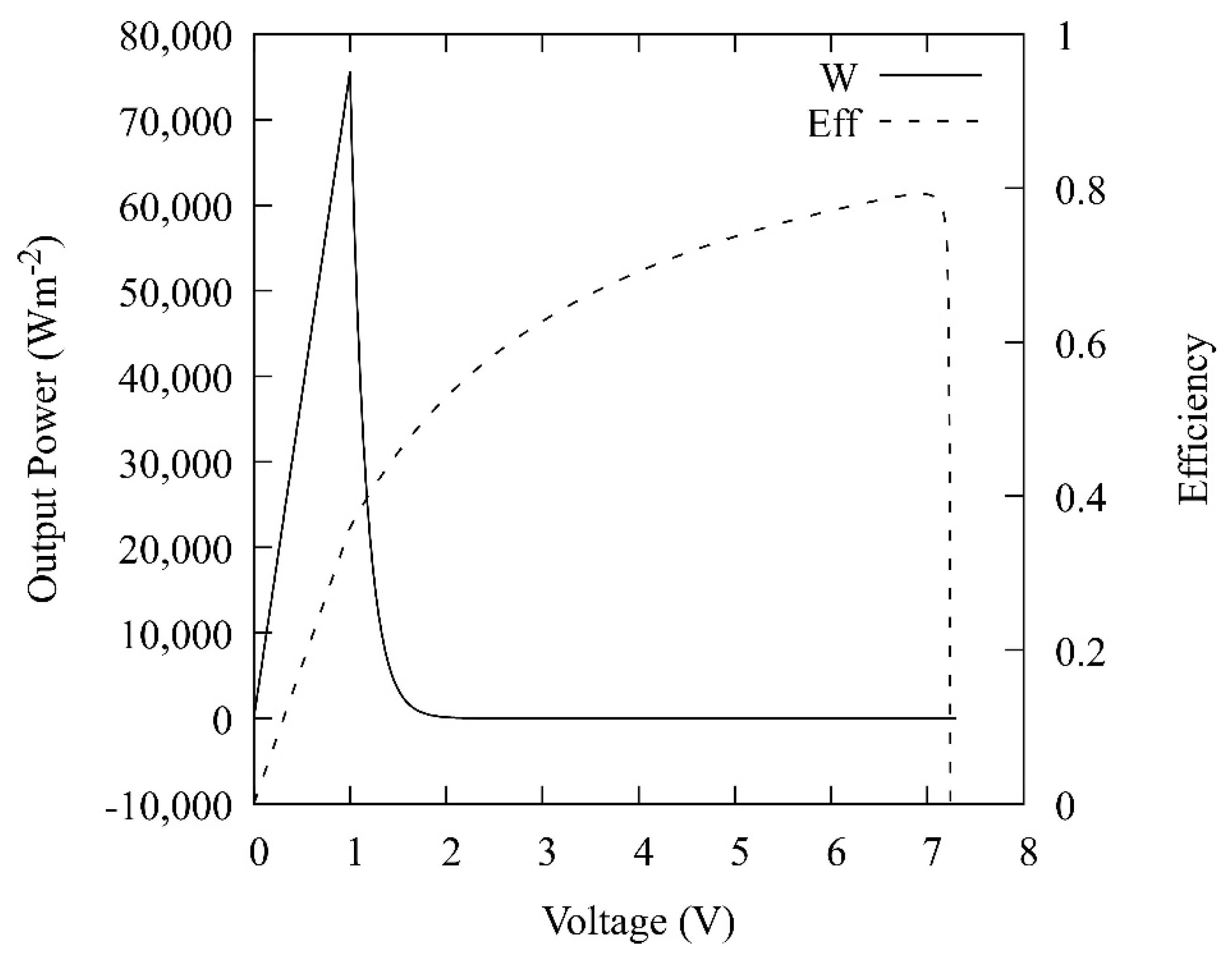
Figure 7 plots the electrical power produced, $\dot{W}$, by the thermionic converter, which is given by:

$$\dot{W}=({\mu }_C-{\mu }_E)({\dot{N}}_{EC}-{\dot{N}}_{CE})$$

(23)

Additionally, the efficiency with which the heat rate supplied to the emitter is converted into electrical power. The derivation of this efficiency will be discussed in the next sections. Contrarily to solar cells, the maximum efficiency is not obtained when the output power is maximum but close to open-circuit conditions. Hence, while open-circuit in this example takes place at 7.235 V, the maximum efficiency (79.24%) takes place at 6.92 V. For reference, we will point out here that the Carnot efficiency for a reversible engine operating between a hot heat reservoir at 1650 K and a cold reservoir at 300 K is 81.82%.

5. Thermodynamic Consistency

Table 1 collects the energy flux $\dot{E}$ and the entropy flux $\dot{S}$ associated to the electron flux calculated in the previous section. The energy flux is obtained from the electron flux by multiplying by the energy of the electron and the entropy flux is obtained through the grand canonical potential flux $\dot{\mathsf{\Omega }}$. The grand canonical potential is the Legendre transform of the energy with respect to the temperature and the electrochemical potential [11]. The logarithmic term appearing in TI.10, for example, is the result of deriving the grand canonical potential from the gran canonical ensemble in the field of statistical mechanics [12]. The derivation of these formulas follows the reasoning in [6] but changing the Bose statistics of photons for the Fermi–Dirac statistics of electrons, the speed of light of the photons by the electron velocity distribution given by Equation (8), as well as by considering the density of states of electrons given by Equation (5) instead of the density distribution of the photon modes.

To analyze the thermodynamic consistency of the model we will consider first the emitter. As detailed in Figure 8, the emitter receives heat ${\dot{Q}}_E$ and emits electrons towards the collector transporting an energy ${\dot{E}}_{EC}$ and entropy ${\dot{S}}_{EC}$ per unit of time. The emitter also receives electrons, not only from the collector, through the vacuum that separates it from the emitter, but also from the electric circuit that connects the emitter and collector through the load. Those traveling through the vacuum transport an energy ${\dot{E}}_{CE}$ and entropy ${\dot{S}}_{CE}$ whilst those coming from the electric circuit inject in the emitter only chemical energy as work ${\dot{W}}_E$, which carries no entropy, and is given by:

$$\dot{W_E}={\mu }_E({\dot{N}}_{EC}-{\dot{N}}_{CE})$$

(24)

Energy conservation (first law of thermodynamics) demands that:

$${\dot{Q}}_E+{\dot{W}}_E={\dot{E}}_{EC}-{\dot{E}}_{CE}$$

(25)

where,

$${\dot{E}}_{EC}=\dot{E}({\mathsf{\Phi }}_E,\infty ,E_{FE},T_E,\pi )eV<{\mathsf{\Phi }}_E-{\mathsf{\Phi }}_C$$

(26)

$${\dot{E}}_{EC}=\dot{E}({\mathsf{\Phi }}_C+eV,\infty ,E_{FE},T_E,\pi )eV>{\mathsf{\Phi }}_E-{\mathsf{\Phi }}_C$$

(27)

is the energy electrons transport from the emitter to the collector and:

$${\dot{E}}_{CE}=\dot{E}({\mathsf{\Phi }}_E,\infty ,eV,T_C,\pi )eV<{\mathsf{\Phi }}_E-{\mathsf{\Phi }}_C$$

(28)

$${\dot{E}}_{EC}=\dot{E}({\mathsf{\Phi }}_C+eV,\infty ,eV,T_C,\pi )eV>{\mathsf{\Phi }}_E-{\mathsf{\Phi }}_C$$

(29)

is the energy that electrons transport from the collector to the emitter.

The second law of thermodynamics states that the conversion process of the heat ${\dot{Q}}_E$ into a flux of electrons transporting energy has to be such that it creates positive or null entropy. Designating this entropy creation rate as ${\dot{S}}_{irr}$ we must assume then that:

$$T_E{\dot{S}}_{irr,E}=T_E{\dot{S}}_{EC}-T_E{\dot{S}}_{CE}-{\dot{Q}}_E\ge 0$$

(30)

where,

$${\dot{S}}_{EC}=\dot{S}({\mathsf{\Phi }}_E,\infty ,E_{FE},T_E,\pi )eV<{\mathsf{\Phi }}_E-{\mathsf{\Phi }}_C$$

(31)

$${\dot{S}}_{EC}=\dot{S}({\mathsf{\Phi }}_C+eV,\infty ,E_{FE},T_E,\pi )eV>{\mathsf{\Phi }}_E-{\mathsf{\Phi }}_C$$

(32)

is the flux of entropy leaving the emitter,

$${\dot{S}}_{CE}=\dot{S}({\mathsf{\Phi }}_E,\infty ,eV,T_C,\pi )eV<{\mathsf{\Phi }}_E-{\mathsf{\Phi }}_C$$

(33)

$${\dot{E}}_{EC}=\dot{E}({\mathsf{\Phi }}_C+eV,\infty ,eV,T_C,\pi )eV>{\mathsf{\Phi }}_E-{\mathsf{\Phi }}_C$$

(34)

is the flux of entropy entering the emitter associated to the flux of electrons coming from the collector and ${\dot{Q}}_E/T_E$ is the flux of entropy associated to the input heat.

Substituting ${\dot{Q}}_E$ from Equation (25) we obtain:

$$T_E{\dot{S}}_{irr,E}=T_E{\dot{S}}_{EC}-T_E{\dot{S}}_{CE}-{\dot{E}}_{EC}+{\dot{E}}_{CE}+{\mu }_E({\dot{N}}_{EC}-{\dot{N}}_{CE})$$

(35)

Figure 9 plots ${\dot{S}}_{irr,E}$ for the case of the thermionic converter whose current–voltage characteristic, power output, and efficiency were exemplified in Figure 6 and Figure 7. As it can be seen, it is verified that ${\dot{S}}_{irr,E}>0$ demonstrating the thermodynamic coherence of the conversion processes taking place in the emitter.

Following a similar approach, we can calculate the production of irreversible entropy at the collector where the energy of the arriving electrons is converted into electrical work ${\dot{W}}_C$, while some energy is dissipated as heat ${\dot{Q}}_C$. The energy conservation of the processes taking place at the collector demands that:

$${\dot{Q}}_C+{\dot{W}}_C={\dot{E}}_{EC}-{\dot{E}}_{CE}$$

(36)

where,

$$\dot{W_C}={\mu }_C({\dot{N}}_{EC}-{\dot{N}}_{CE})$$

(37)

The fulfillment of the second law requires that:

$$T_C{\dot{S}}_{irr,C}=T_C{\dot{S}}_{CE}-T_C{\dot{S}}_{EC}+{\dot{Q}}_C\ge 0$$

(38)

where ${\dot{Q}}_C$ is obtained from Equation (36). Figure 9 plots also ${\dot{S}}_{irr,C}$ for the case of the thermionic converter whose current–voltage characteristic, power output, and efficiency $\eta$, defined as:

$$\eta =\frac{\dot{W}}{\dot{Q_E}}=\frac{\dot{W_C}-\dot{W_E}}{\dot{Q_E}}$$

(39)

were exemplified in Figure 6 and Figure 7, verifying that ${\dot{S}}_{irr,C}$ > 0.

6. Conclusions

We have calculated the energy and entropy fluxes associated to the electron fluxes involved in the Richardson–Duhmann model for the thermionic converter and with them, verified that the model is consistent with the second principle of thermodynamics in which entropy creation must be zero or positive. In the review of the model, we have generalized it to take into account Fermi–Dirac statistics and have pointed out the importance of referring the calculations to a point in between the emitter and the collector (point A) in which the electric field is zero. It is at this point where it is possible to assume that the electrons are free and, therefore, we can calculate their density of states as free electrons. It is also therefore at this point at which the electron, energy, and entropy fluxes going from the emitter to the collector and vice-versa must be calculated. When the voltage at the collector is such that $eV<{\mathsf{\Phi }}_E-{\mathsf{\Phi }}_C$, this point is close to the emitter and due to this proximity it is assumed that electrons, when travelling to the emitter preserve their emitter temperature and chemical potential; when the voltage at the collector is such that $eV>{\mathsf{\Phi }}_E-{\mathsf{\Phi }}_C$ this point is close to the collector and, similarly, it is assumed that electrons, when travelling to the collector from the emitter preserve their collector temperature and chemical potential.