Abstract
The effective thermal conductivity (λeff) of sands is a critical parameter required by applications in geothermal energy resources, geo-technique and geo-environment and in science disciplines. However, the availability of the reliable λeff data is not sufficient and predictive models are usually used in practice to estimate λeff. These predictive models may vary in complexity, flexibility, accuracy and applications. There is no universal model that can be applied to all soil types and full water content range. The choice of different models may result in distinctive estimates of λeff. The objectives of this study were to conduct an extensive review of the thermal conductivity models of sands and evaluate their performance with a large dataset consisting of various sand types from dry to saturation. A total of 14 models to predict λeff of sands were evaluated with a large compiled dataset consisting of 1025 measurements on 62 sands from 20 studies. The results show that the models of Chen 2008 (CS2008) and Zhang et al. 2016 (ZN2016) give the best estimates of thermal conductivity of sands, with Nash–Sutcliffe efficiency = 0.9 and RMSE = 0.3 W m−1 °C−1. These two models are potentially applied to accurately estimate thermal conductivity of sands of different types.
1. Introduction
The effective thermal conductivity (λeff, W m−1 °C−1) of sands is of great interest because it is required by petroleum or natural gas production from underground oil- or methane-bearing sands [1,2]. It is also the critical parameter to determine heat exchange between the surrounding environments and the borehole heat exchanger [3,4,5,6], nuclear waste disposal [7] or energy storage [8], buried power cables and steam/hot water pipelines [9], and other thermo-active ground structures (e.g., energy pile and tunnel linings). The value of λeff is often an input for calculating the ground thermal regimes or land-atmosphere energy balance and associated soil physical, chemical and biological processes [10,11].
The values of λeff can be either measured or indirectly predicted with mathematic models. The available λeff data of sands are not sufficient to meet the demands, although great progress has been achieved in the measurement technologies of λeff [12,13,14]. In addition, reliable λeff data can only be measured by the transient method (e.g., heat pulse method) at full water content range, because the transient method is less likely to be affected by the water redistribution or phase change compared to the steady-state method (e.g., guarded hot plate). On the other hand, modeling of λeff is a highly thriving field, because there is no single model for universal applications. Previous studies generally applied models of other applications to estimate λeff of sands, while some developed predictive models for sands but based on a small size dataset [15,16] or unreliable measurements [17]. The complexity, flexibility, accuracy and applications of the predictive models largely determine the accuracy of their applications [18,19]. Therefore, it is critical to evaluate the performance of the predictive models for sands for accurate applications in engineering and science.
The objectives of this study were: (1) to conduct an extensive review of the predictive thermal conductivity models of sands; (2) to compile a large and reliable dataset consisting of measurements on various sands at full water content range with the transient heat pulse methods; and (3) to evaluate the performance of the collated models with the compiled dataset.
2. A Review of STC Models for Sands
2.1. Overview of Soil Thermal Conductivity Models for Sands
An extensive literature search gives 14 models that were originally developed to predict thermal conductivity of sands. The 14 models are divided into three categories, including six mixing or analytical models, four models based on the normalized concept and four linear/non-linear regression models. The models of Woodside and Messmer [1] (WM1961I, WM1961II) and Tarnawski and Leong [20] (TL2016) are original or modified geometric mean models and that of Lu et al. [21] (LY2018) is a mixed series and parallel model. The Haigh [16] (HS2012) and Rubin and Ho [22] (RH2018) models are physically based models. The Ewen and Thomas [23] (ET1987), Zhang et al. [24] (ZN2015), Zhang et al. [25] (ZN2016) and Zhao et al. [26] (ZY2019) models are normalized thermal conductivity models. The Becker et al. [27] (BB1992), Chen [15] (CS2008), Li et al. [28] (LY2012) and Alrtimi et al. [17] (AA2016) models were developed empirically.
2.2. Analytical or Mixing Models
2.2.1. Woodside and Messmer 1961 Model (WM1961I)
Woodside and Messmer [1] presented the classical weighted geometric mean model to calculate λeff of 2-phase saturated sands. The geometric mean model was extended for a three-phase soil system [29,30]
where P is porosity (cm3 cm−3), θ is water content (cm3 cm−3), λs, λw and λair are thermal conductivity of soil solids, water and air (W m−1 °C−1). λw = 0.56 W m−1 °C−1 and λair = 0.025 W m−1 °C−1 are assumed.
2.2.2. Woodside and Messmer 1961 Model (WM1961II)
Woodside and Messmer [1] also presented another model similar to the geometric mean model [31,32,33]
2.2.3. Tarnawski and Leong 2016 Model (TL2016)
Kiyohashi and Deguchi [30] were among the first to extend Equation (1) of Woodside and Messmer [1] to unsaturated solid rocks (e.g., sandstones, zeolites, tuff, etc.) with 0.05 < n < 0.51 (with accuracy of λeff = ±0.20 W m−1 °C−1)
Tarnawski and Leong [20] found Equation (3) overestimates λeff of unsaturated soils due to the model is lack of physical characteristics for unsaturated soil applications. They introduced the inter-particle thermal contact resistance factor (α)
where α is expressed as [20,34,35]
where Sr−cr is the degree of saturation of a miniscule pore space, Sr−cr = (0.22fclay + 0.01)/P [20,36], ε is a dimensionless interface contact coefficient (0 ≤ ε ≤ 1, ε = 1 indicates an ideal contact between soil particles). ε depends on soil compaction, soil specific surface area, and grain size distribution. Tarnawski and Leong [20] obtained ε value by reverse modeling of experimental λeff data of 40 Canadian soils; the resulting ε varied between 0.988 and 0.994 for coarse and fine soils, respectively. For dry soils, α ᾰ1 due to the highest λ reduction arising from the thermal contact resistance.
2.2.4. Haigh 2012 Model (HS2012)
Based on dataset of Chen [15], Haigh [16] developed an analytical model based on unidirectional heat flow through a three-phase soil system [17,37],
where F = 1.58 is a correction factor, and are thermal conductivity of water (λw, W m−1 °C−1) and air (λair, W m−1 °C−1), respectively, that are divided by λs
where coefficients a and b are related to the thickness of water film and degree of saturation
where e is the void ratio, e = P/(1 − P). The left side of Equation (10) can be simplified as , and .
2.2.5. Lu Et Al. 2018 Model (LY2018)
Lu et al. [21] developed a parallel-series mixed model for predicting λeff of Aeolian sand on the Qinghai-Tibet Plateau
where a and b are fitting parameters. Lu et al. [21] recommended a = 0.76 and b = 1 for unfrozen soils and a = 0.72 and b = 2.06 for frozen soils.
2.2.6. Rubin and Ho 2018 Model (RH2018)
Rubin and Ho [22] showed that the Haigh [16] model underestimates λeff and they provided an alternative empirical equation for the correction factor F [38]
where x is the estimated λeff with the Haigh [16] model when F = 1, multiplying the λeff calculating with Haigh [16] by the F gives the corrected λeff. The R2 for Equation (12a,b) are 0.65 and 0.87, respectively.
2.3. Normalized Models
2.3.1. Ewen and Thomas 1987 Model (ET1987)
Ewen and Thomas [23] proposed a modified Johansen [39] model
where λsat and λdry are thermal conductivities when soil is saturated or dry, respectively. Ke is an exponential function that is dependent on degrees of saturation. Ke is calculated by [23]
where ξ is a fitted parameter, ξ = 8.9 was recommended by Ewen and Thomas [23] which returns Ke ≈ 1 at Sr = 1. .
Values of λsat and λdry are calculated by a two-phase system (solid-air or solid-water) [39]
where θl is the unfrozen water content (cm3 cm−3), λw is the thermal conductivity of water, λw = 0.56 W m−1 °C−1 at above-zero temperature, λw = 0.269 W m−1 °C−1 at sub-zero temperature [40], λice is the thermal conductivity of ice (2.2 W m−1 °C−1), ρb is the bulk density (g cm−3), λs is the thermal conductivity of the solid that can be calculated based on volumetric fraction and thermal conductivity of quartz (fquartz, λquartz) and other minerals (λother),
where λq = 7.7 W m−1 °C−1 and λother = 2.0 W m−1 °C−1 for fq > 20% and λother = 3 for fq ≤ 20% at 20 °C.
2.3.2. Zhang Et Al. 2015 Model (ZN2015)
Zhang et al. [24] modified the Côté and Konrad [41] model by introducing a different set of parameters with k = 6.0, χ = 8.12 W m−1 °C−1, and η = 3.28 for quartz sand. The modified model becomes [24]
2.3.3. Zhang Et Al. 2016 Model (Z2016)
Zhang et al. [25] further modified the Côté and Konrad [41] model with experimental data measured on sand-kaolin clay mixtures with thermo-TDR method, the resulting formula is
where λkaolin is thermal conductivity of kaolin (2.9 W m−1 °C−1), Kaolin is assumed to be zero in this study. Equation (16) is used to calculate λs.
2.3.4. Zhao Et Al. 2019 Model (ZY2019)
Zhao et al. [26] presented a closed-form thermal conductivity model for mixtures of sands and peat materials
where A and B are parameters related to soil properties (composition, texture and structure)—they can be directly derived from the lower and upper water saturations. λeff = λdry = A when Sr = 0 and B = (λsat − λdry)/Ln2 when Sr = 1. Equation (20) can be converted to the normalized form as Ke = Log2 (1 + Sr)
where Equations (15a), (16) and (17a) are retained for calculation of λsat, λs and λdry, respectively.
2.4. Linear or Nonlinear Regression Models
2.4.1. Becker 1992 Model (BB1992)
Becker et al. [27] developed an unified methodology for predicting λeff of gravel, sand, silt, clay and peat in both frozen and unfrozen states using literature data [42]
or
where UC = 0.1442 is used to convert the SI unit (W m−1 °C−1) back to “Btu in. ft−2 h−1 °F−1” for consistence with the original study. a1 to a4 are coefficients depending on soil type. For unfrozen sand, a1 to a4 are 6.8, 0.4, −2.9 and −1.5, respectively.
2.4.2. Chen 2008 Model (CS2008)
Chen [15] proposed a simple empirical relationship for sandy soils
where b = 0.0022 and c = 0.78 are the fitting parameters obtained using DPS code with R2 = 0.996, λs is calculated with Equation (16).
2.4.3. Li Et Al. 2012 Model (LY2012)
Li et al. [28] developed an empirical relationship for powdery sand while test soil thermal conductivity along a crude oil pipeline in tropical desert and grassland in southwest Sahara Desert in West Africa,
2.4.4. Alrtimi Et Al. 2016 Model (AA2016)
Alrtimi et al. [17] developed a new logarithmic expression for sands:
3. Data Compilation and Analysis
3.1. Experimental Data of Thermal Conductivity of Sand
A large dataset was collated by digitaltizing literature data or by collecting through personal communications following several important criteria: (1) soil must be sands with zero or a negligibly small amount of organic matter. Full dataset of Chen [15] was included because it has been used by a few researchers to compare, develop, or test new models [16,18,22,38], additional soils contain sand content ~>90%; (2) λeff were measured on soil samples with the transient method (e.g., single/dual-probe heat pulse method, thermo-TDR) at room temperature; (3) sufficient sample size and a wide range of water contents or degrees of saturation (e.g., >5) and bulk densities should be provided for useful evaluation; and (4) detailed description of the sample preparation and complete soil information such as grain size distribution (fsand, fsilt, and fclay), P, ρb, and ρs should be available. The values of λs and fq that were measured or recommended by original research were used, otherwise fq = fsand is assumed and missed λs was calculated by Equation (16).
This screen procedure ended up with 1025 measurements on 62 sands from 20 studies [9,15,23,25,26,36,43,44,45,46,47,48,49,50,51,52,53,54,55,56,57], which are all published data. These data were mainly measured under controlled laboratory conditions to maintain high quality. The sand samples of this compiled dataset were from different regions around the world, including Germany [43], the UK [23], Greece [52], Australia [44], the USA [25,36,45,51,57], Canada [26,53,54,55,56], China [15,46], Japan [47,50] and South Korea [9]. Selected soil physical properties can be found in Table 1. Detailed information can be found in the respective studies.

Table 1.
Selected Physical Properties of Soils for Model Evaluation.
3.2. Performance Metrics
The similarity between the predicted and actual values was assessed by plotting them on a 1:1 diagram with ±10% line and two goodness-of-fit parameters were used, including (1) root mean square error (RMSE)
and (2) Nash-Sutcliffe efficiency (NSE):
where is the jth measured value, is the jth predicted value, is the mean of measured values, and n is the number of measured values. NSE = 1 indicates a perfect match between and ; NSE = 0 indicates that is as accurate as ; while NSE < 0 indicates that is a better predictor. RMSE indicates the absolute difference between and —the closer the RMSE value is to zero, the better the predictor.
4. Results and Discussion
4.1. Analytical or Mixing Models
The best performing model among the six thermal conductivity models of this category is TL2016 (Table 2 and Figure 1(3)) with RMSE = 0.43 W m−1 °C−1 and NSE = 0.79. The HS2012 (Figure 1(4)) model retains a physical origin but it is relatively complex [17,37] and does not have a satisfactory performance on the dataset investigated. The models of TL2016 (Figure 1(3)) and WM1961I (Figure 1(1)) generally underestimate the measured λeff. The WM1961II (Figure 1(2)), LY2018 (Figure 1(5)) and RH2018 (Figure 1(6)) generally overestimate the measured λeff.
Table 2.
Performance metrics of the 14 thermal conductivity models for sands.
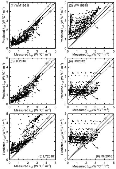
Figure 1.
Comparison of measured λeff and predicted λeff with six analytical or mixing models: (1) WM1961I [1], (2) WM1961II [1], (3) TL2016 [20], (4) HS2012 [16], (5) LY2018 [21] and (6) RH2018 [22].
The WM1961I and WM1961II were originally developed for water saturated soils with λs/λw ≈ 10 [1]. Although the geometric mean model was extended for frozen soil study by Cosenza et al. [31] and Endrizzi et al. [32], and incorporated into the GEOtop program [33], the extension to three-phase system may not always be valid because this model lacks a physical basis for the heat conduction in granular materials [58,59]. The LY2018 model was developed based on the basic series-parallel model using a small dataset (28 measurements) of Aeolian sands from the Tibetan Plateau [21]. The RH2018 model (Figure 1(6)) is in fact the modified form of HS2012 (Figure 1(4)) model by multiplying an F factor based on Equation (12). However, it should be noted that Equation (12a) gave an unreasonably high value at Sr < 0.1 and only Equation (12b) was used for all degrees of saturation in this study. Rubin and Ho [22] found that the correction factor worked well for the dataset of Chen [15] and others (a total of 155 measurements), but a large variation was reported when applying this method to their own measurements (124 measurements). Therefore, it is not surprising to see that it showed a greater variation on a much larger dataset used in this study (a total of 1025 measurements).
4.2. Normalized Models
The four normalized thermal conductivity models generally performed better than the analytical or mixing models of Section 4.1. The ZN2016 (Table 2, Figure 2(3)) performed the best, with RMSE = 0.3 W m−1 °C−1 and NSE = 0.9, followed by ZN2015 (Table 2, Figure 2(2)), with RMSE = 0.33 W m−1 °C−1 and NSE = 0.88. It should be noted that both models, ZN2015 and ZN2016, are a modified form of the Côté and Konrad [41] model. The difference is that the ZN2015 model was developed for quartz sand while the ZN2016 was developed for a sand-clay mixture [24,25]. The normalized thermal conductivity models are among the most prevalent soil thermal conductivity models, because they generally give satisfactory estimates [19,60]. The ZN2015 and ZN2016 models extend the capability of the normalized thermal conductivity model to accurately predict λeff of sands at a high range of λeff (or water content range), but they still faced difficulties in λeff prediction at low to middle ranges of λeff. The ET1987 model (Figure 2(1)) generally overestimated the measured λeff, which agrees with the findings of other research [18,19]. The ZY2019 model (Figure 2(4)) generally slightly underestimated measured λeff, the same underestimates was reported by previous study [19]. The possible reason for the underestimates of the ZY2019 model is that it was developed for a sand-peat mixture, in which peat has a much smaller magnitude of thermal conductivity [26].
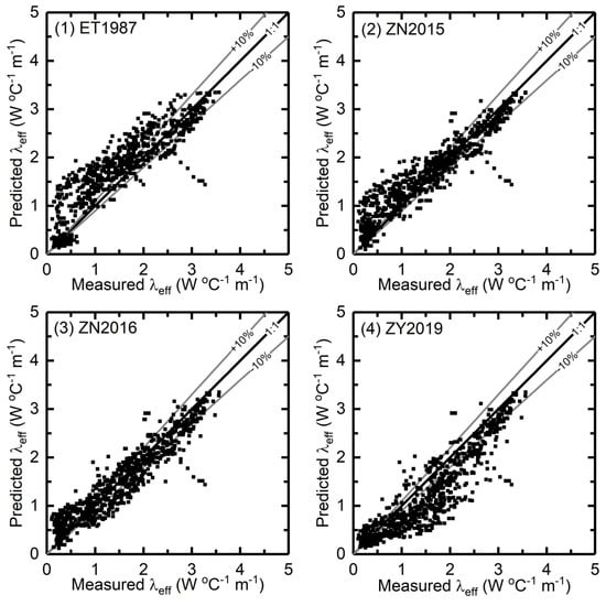
Figure 2.
Comparison of measured λeff and predicted λeff with four normalized thermal conductivity models: (1) ET1987 [23], (2) ZN2015 [24], (3) ZN2016 [25] and (4) ZY2019 [26].
4.3. Linear or Non-Linear Regression Models
The CS2008 model (Figure 3(2)) is the best performing model in this category and performs equally well with model of ZN2016. The CS2008 model was developed empirically for estimating λeff of quartz sands, but it actually has a form similar to that of the geometric mean model [1,39,61]. The inclusion of λs may explain why it outperformed the other three empirical models (i.e., BB1992, LY2012 and AA2016) in this category. The BB1992 (Figure 3(1)) and LY2012 (Figure 3(3)) models have mixed performance, giving overestimates of λeff at ranges below ~1 W m−1 °C−1 and underestimates of λeff at ranges greater than ~1 W m−1 °C−1. The LY2012 model was developed for powdery sand in tropical desert and grassland in the southwest Sahara Desert in West Africa [28]—the sand characteristics may different from sands from other parts of the world. This difference may result in the unsatisfactory performance of the LY2012 model. The AA2016 model (Figure 3(4)) generally overestimated the measured λeff as a whole, which may be attributed to the fact that AA2016 was developed based on steady-state measurements (i.e., guarded hot plates). Steady-state measurements are prone to water redistribution in unsaturated soils, which changes the thermal conductivity being measured [12,62]. This may explain why Alrtimi et al. [17] found that the models of de Vries [63], Johansen [39], Côté and Konrad [41], Lu et al. [48], Chen [15] and Haigh [16] could not be used to properly predict thermal conductivity of Tripoli sand measured with the steady-state measurements. Therefore, care should be taken when applying these models.
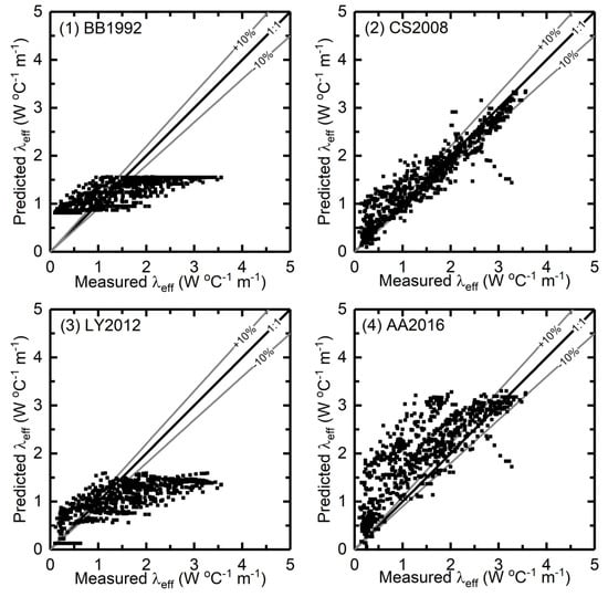
Figure 3.
Comparison of measured λeff and predicted λeff with four linear or non-linear regression models: (1) BB1992 [27], (2) CS2008 [15], (3) LY2012 [28] and (4) AA2016 [17].
5. Conclusions
In this study, 14 models used to predict the thermal conductivity of sands were reviewed and evaluated with a large compiled dataset consisting of 1025 thermal conductivity measurements measured on 62 sands from 20 studies. The results show that most of the models either underestimated or overestimated the experimental measurements. Only the models of Chen [15] (CS2008) and Zhang et al. [25] (ZN2016) gave the best estimates, with Nash-Sutcliffe efficiency = 0.9 and RMSE = 0.3 W m−1 °C−1. These two models can potentially be used for accurately estimating the thermal conductivity of sands of different types with satisfactory performance. Although sands from various locations around the world were used in this study, care should be taken when applying the selected models for much wider applications beyond the sands tested due to the highly spatial variability in the nature of soil properties. This work would provide useful information pertaining to applications in geothermal energy resources, geo-techniques and geo-environments and in science disciplines that require the effective thermal conductivity of sands.
Author Contributions
Manuscript preparation: J.W. and H.H.; Data analysis and graph: J.W.; Revision of the manuscript: H.H., M.D. and J.L. All authors have read and agreed to the published version of the manuscript.
Funding
Funding for this research was provided in part by the National Key Research and Development Program of China (No. 2017YFD0200205), National Natural Science Foundation of China (NSFC, Grant No. 41877015), China Postdoctoral Science Foundation (2018M641024), the Northwest A&F University, and the 111 project (No. B12007).
Acknowledgments
Datasets used in this study were digitalized from the published literature or colleted through personal communication, the authors are indebted to their work and efforts for taking these measurements. Special thanks go to Yingying Chen, Sen Lu, Yili Lu, and Ying Zhao for providing their dataset.
Conflicts of Interest
The authors declare no conflict of interest.
References
- Woodside, W.; Messmer, J.H. Thermal conductivity of porous media. I. Unconsolidated sands. J. Appl. Phys. 1961, 32, 1688–1699. [Google Scholar] [CrossRef]
- Waite, W.F.; deMartin, B.J.; Kirby, S.H.; Pinkston, J.; Ruppel, C.D. Thermal conductivity measurements in porous mixtures of methane hydrate and quartz sand. Geophys. Res. Lett. 2002, 29, 81–84. [Google Scholar] [CrossRef]
- Wang, H.; Cui, Y.; Qi, C. Effects of sand–bentonite backfill materials on the thermal performance of borehole heat exchangers. Heat Transf. Eng. 2013, 34, 37–44. [Google Scholar] [CrossRef]
- Zhang, X.; Zhang, T.; Li, B.; Jiang, Y. Comparison of four methods for borehole heat exchanger sizing subject to thermal response test parameter estimation. Energies 2019, 12, 4067. [Google Scholar] [CrossRef]
- Baglivo, C.; D’Agostino, D.; Congedo, P.M. Design of a ventilation system coupled with a horizontal air-ground heat exchanger (haghe) for a residential building in a warm climate. Energies 2018, 11, 2122. [Google Scholar] [CrossRef]
- Sáez Blázquez, C.; Farfán Martín, A.; Martín Nieto, I.; Gonzalez-Aguilera, D. Measuring of thermal conductivities of soils and rocks to be used in the calculation of a geothermal installation. Energies 2017, 10, 795. [Google Scholar] [CrossRef]
- Yoon, S.; Cho, W.; Lee, C.; Kim, G.-Y. Thermal conductivity of Korean compacted bentonite buffer materials for a nuclear waste repository. Energies 2018, 11, 2269. [Google Scholar] [CrossRef]
- Ertas, A.; Boyce, C.T.R.; Gulbulak, U. Experimental measurement of bulk thermal conductivity of activated carbon with adsorbed natural gas for ang energy storage tank design application. Energies 2020, 13, 682. [Google Scholar] [CrossRef]
- Sohn, B.-H. Thermal conductivity measurement of sand-water mixtures used for backfilling materials of vertical boreholes or horizontal trenches. Korean J. Air Cond. Refrig. Eng. 2008, 20, 342–350. [Google Scholar]
- He, H.; Dyck, M.; Si, B.; Zhang, T.; Lv, J.; Wang, J. Soil freezing–thawing characteristics and snowmelt infiltration in cryalfs of Alberta, Canada. Geoderma Reg. 2015, 5, 198–208. [Google Scholar] [CrossRef]
- Peters-Lidard, C.D.; Blackburn, E.; Liang, X.; Wood, E.F. The effect of soil thermal conductivity parameterization on surface energy fluxes and temperatures. J. Atmos. Sci. 1998, 55, 1209–1224. [Google Scholar] [CrossRef]
- He, H.; Dyck, M.; Horton, R.; Ren, T.; Bristow, K.L.; Lv, J.; Si, B. Development and application of the heat pulse method for soil physical measurements. Rev. Geophys. 2018, 56, 567–620. [Google Scholar] [CrossRef]
- Palacios, A.; Cong, L.; Navarro, M.E.; Ding, Y.; Barreneche, C. Thermal conductivity measurement techniques for characterizing thermal energy storage materials—A review. Renew. Sustain. Energy Rev. 2019, 108, 32–52. [Google Scholar] [CrossRef]
- He, H.; Dyck, M.; Horton, R.; Li, M.; Jin, H.; Si, B. Distributed Temperature Sensing for Soil Physical Measurements and its Similarity to Heat Pulse Method. In Advances in Agronomy; Sparks, D.L., Ed.; Academic Press: Cambridge, UK, 2018; Volume 148, pp. 173–230. [Google Scholar]
- Chen, S. Thermal conductivity of sands. Heat and Mass Transf. 2008, 44, 1241–1246. [Google Scholar] [CrossRef]
- Haigh, S.K. Thermal conductivity of sands. Géotechnique 2012, 62, 617–625. [Google Scholar] [CrossRef]
- Alrtimi, A.; Rouainia, M.; Haigh, S. Thermal conductivity of a sandy soil. Appl. Therm. Eng. 2016, 106, 551–560. [Google Scholar] [CrossRef]
- He, H.; Zhao, Y.; Dyck, M.; Si, B.; Jin, H.; Lv, J.; Wang, J. A modified normalized model for predicting effective soil thermal conductivity. Acta Geotech. 2017, 12, 1281–1300. [Google Scholar] [CrossRef]
- He, H.; Noborio, K.; Johansen, Ø.; Dyck, M.; Lv, J. Normalized concept for effective soil thermal conductivity modelling from dryness to saturation. Eur. J. Soil Sci. 2020, 71, 27–43. [Google Scholar] [CrossRef]
- Tarnawski, V.R.; Leong, W.H. Advanced geometric mean model for predicting thermal conductivity of unsaturated soils. Int. J. Thermophys. 2016, 37, 18. [Google Scholar] [CrossRef]
- Lu, Y.; Yu, W.; Hu, D.; Liu, W. Experimental study on the thermal conductivity of Aeolian sand from the Tibetan plateau. Cold Reg. Sci. Technol. 2018, 146, 1–8. [Google Scholar] [CrossRef]
- Rubin, A.J.; Ho, C.L. A Modified Method for Estimating the Thermal Conductivity of Sands. In Proceedings of the GeoShanghai 2018 International Conference: Transportation Geotechnics and Pavement Engineering, Shangha, China, 27–30 May 2018. [Google Scholar]
- Ewen, J.; Thomas, H.R. The thermal probe—A new method and its use on an unsaturated sand. Géotechnique 1987, 37, 91–105. [Google Scholar] [CrossRef]
- Zhang, N.; Yu, X.; Pradhan, A.; Puppala, A.J. Thermal conductivity of quartz sands by thermo-time domain reflectometry probe and model prediction. J. Mater. Civ. Eng. 2015, 27, 04015059. [Google Scholar] [CrossRef]
- Zhang, N.; Yu, X.; Pradhan, A.; Puppala, A.J. A new generalized soil thermal conductivity model for sand–kaolin clay mixtures using thermo-time domain reflectometry probe test. Acta Geotech. 2016, 12, 739–752. [Google Scholar] [CrossRef]
- Zhao, Y.; Si, B.C.; Zhang, Z.; Li, M.; He, H.; Hill, L.R. A new thermal conductivity model for sandy and peat soils. Agric. For. Meterol. 2019, 274, 95–105. [Google Scholar] [CrossRef]
- Becker, B.R.; Misra, A.; Fricke, B.A. Development of correlations for soil thermal conductivity. Int. Commun. Heat Mass Transf. 1992, 19, 59–68. [Google Scholar] [CrossRef]
- Li, Y.; Wu, C.; Xing, X.; Yue, M.; Shang, Y. Testing and Analysis of the soil Thermal Conductivity in Tropical Desert and Grassland of West Africa. In Proceedings of the 2012 9th International Pipeline Conference, Calgary, AB, Canada, 24–28 September 2012; American Society of Mechanical Engineers: New York, NY, USA, 2012; pp. 149–157. [Google Scholar]
- Judge, A.S. The Thermal Regime of the Mackenzie Valley: Observations of the Natural State; Environmental-Social Committee, Northern Pipelines, Task Force on Northern Oil Development: Ottawa, ON, Canada, 1973. [Google Scholar]
- Kiyohashi, H.; Deguchi, M. Derivation of a correlation formula for the effective thermal conductivity of geological porous materials by the three-phase geometric-mean model. High Temp. High Press. 1998, 30, 25–35. [Google Scholar] [CrossRef]
- Cosenza, P.; Guérin, R.; Tabbagh, A. Relationship between thermal conductivity and water content of soils using numerical modelling. Eur. J. Soil Sci. 2003, 54, 581–588. [Google Scholar] [CrossRef]
- Endrizzi, S.; Quinton, W.L.; Marsh, P. Modelling the spatial pattern of ground thaw in a small basin in the arctic tundra. Cryosphere Discuss 2011, 2011, 367–400. [Google Scholar] [CrossRef]
- Endrizzi, S.; Gruber, S.; Dall’Amico, M.; Rigon, R. Geotop 2.0: Simulating the combined energy and water balance at and below the land surface accounting for soil freezing, snow cover and terrain effects. Geosci. Model Dev. 2014, 7, 2831–2857. [Google Scholar] [CrossRef]
- Tarnawski, V.R.; Leong, W.H.; Gori, F.; Buchan, G.D.; Sundberg, J. Inter-particle contact heat transfer in soil systems at moderate temperatures. Int. J. Energy Res. 2002, 26, 1345–1358. [Google Scholar] [CrossRef]
- Sundberg, J. Thermal Properties of Soils and Rocks; Chalmers University of Technology and University of Gothenburg: Gothenburg, Sweden, 1988. [Google Scholar]
- McInnes, K.J. Thermal Conductivities of Soils from Dryland Wheat Regions of Eastern Washington; Washington State University: Washington, DC, USA, 1981. [Google Scholar]
- Zhang, N.; Yu, X.; Wang, X. Use of a thermo-tdr probe to measure sand thermal conductivity dryout curves (tcdcs) and model prediction. Int. J. Heat Mass Transf. 2017, 115, 1054–1064. [Google Scholar] [CrossRef]
- Rubin, A.J.; Ho, C.L. A Review of Two Methods to Model the Thermal Conductivity of Sands. In Proceedings of the Geotechnical Frontiers 2017, Orlando, FL, USA, 12–15 March 2017. [Google Scholar]
- Johansen, O. Varmeledningsevne av Jordarter (Thermal Conductivity of Soils). In CRREL Draft English Translation 637; University of Trondheim: Trondheim, Norway; US Army Corps of Engineers, Cold Regions Research and Engineering Laboratory: Hanover, NH, USA, 1975. [Google Scholar]
- Yamazaki, Y.; Tsuchiya, F.; Tsuji, O. Measurement and estimation of thermal conductivity of quartz-containing frozen and unfrozen soils (in Japanese with English abstract). Trans. Jpn. Soc. Irrig. Drain. Reclam. Eng. 2003, 226, 497–505. [Google Scholar]
- Côté, J.; Konrad, J.-M. A generalized thermal conductivity model for soils and construction materials. Can. Geotech. J. 2005, 42, 443–458. [Google Scholar] [CrossRef]
- Dissanayaka, S.H.; Hamamoto, S.; Kawamoto, K.; Komatsu, T.; Moldrup, P. Thermal properties of peaty soils: Effects of liquid-phase impedance factor and shrinkage. Vadose Zone J. 2012, 11. [Google Scholar] [CrossRef]
- Bachmann, J.; Horton, R.; Ren, T.; van der Ploeg, R.R. Comparison of the thermal properties of four wettable and four water-repellent soils. Soil Sci. Soc. Am. J. 2001, 65, 1675–1679. [Google Scholar] [CrossRef]
- Barry-Macaulay, D.; Bouazza, A.; Singh, R.M.; Wang, B.; Ranjith, P.G. Thermal conductivity of soils and rocks from the Melbourne (Australia) region. Eng. Geol. 2013, 164, 131–138. [Google Scholar] [CrossRef]
- Cass, A.; Campbell, G.S.; Jones, T.L. Enhancement of thermal water-vapor diffusion in soil. Soil Sci. Soc. Am. J. 1984, 48, 25–32. [Google Scholar] [CrossRef]
- Chen, Y.; Yang, K.; Tang, W.; Qin, J.; Long, Z. Parameterizing soil organic carbon’s impacts on soil porosity and thermal parameters for eastern Tibet grasslands. Sci. China Earth Sci. 2012, 55, 1001–1011. [Google Scholar] [CrossRef]
- Kasubuchi, T.; Momose, T.; Tsuchiya, F.; Tarnawski, V. Normalized thermal conductivity model for three Japanese soils. Trans. Jpn. Soc. Irrig. Drain. Rural Eng. 2007, 251, 529–533. [Google Scholar]
- Lu, S.; Ren, T.; Gong, Y.; Horton, R. An improved model for predicting soil thermal conductivity from water content at room temperature. Soil. Sci. Soc. Am. J. 2007, 71, 8–14. [Google Scholar] [CrossRef]
- Lu, Y.; Wang, Y.; Ren, T. Using late time data improves the heat-pulse method for estimating soil thermal properties with the pulsed infinite line source theory. Vadose Zone J. 2013, 12, 0011. [Google Scholar] [CrossRef]
- Mochizuki, H.; Sakaguchi, I.; Inoue, M. Comparison of the methods measuring of soil thermal conductivity (in Japanese with English abstract). J. Jpn. Soc. Soil Phys. 2003, 93, 47–50. [Google Scholar]
- Park, S.-I.; Hartley, J.G. A model for prediction of the effective thermal conductivity of granular materials with liquid binder. KSME J. 1992, 6, 88–94. [Google Scholar] [CrossRef]
- Papadakis, G.; Glaglaras, P.; Kyritsis, S. A numerical method for determining thermal conductivity of porous media from in-situ measurements using a cylindrical heat source. J. Agric. Eng. Res. 1990, 45, 281–293. [Google Scholar] [CrossRef]
- Tarnawski, V.R.; Momose, T.; Leong, W.H.; Bovesecchi, G.; Coppa, P. Thermal conductivity of standard sands. Part i. Dry-state conditions. Int. J. Thermophys. 2009, 30, 949–968. [Google Scholar] [CrossRef]
- Tarnawski, V.R.; Momose, T.; Leong, W.H. Thermal conductivity of standard sands ii. Saturated conditions. Int. J. Thermophys. 2011, 32, 984–1005. [Google Scholar] [CrossRef]
- Tarnawski, V.R.; McCombie, M.L.; Momose, T.; Sakaguchi, I.; Leong, W.H. Thermal conductivity of standard sands. Part iii. Full range of saturation. Int. J. Thermophys. 2013, 34, 1130–1147. [Google Scholar] [CrossRef]
- Tarnawski, V.R.; Momose, T.; McCombie, M.L.; Leong, W.H. Canadian field soils iii. Thermal-conductivity data and modeling. Int. J. Thermophys. 2015, 36, 119–156. [Google Scholar] [CrossRef]
- Smits, K.M.; Sakaki, T.; Limsuwat, A.; Illangasekare, T.H. Thermal conductivity of sands under varying moisture and porosity in drainage–wetting cycles. Vadose Zone J 2010, 9, 172–180. [Google Scholar] [CrossRef]
- Rees, S.W.; Adjali, M.H.; Zhou, Z.; Davies, M.; Thomas, H.R. Ground heat transfer effects on the thermal performance of earth-contact structures. Renew. Sustain. Energy Rev. 2000, 4, 213–265. [Google Scholar] [CrossRef]
- Béhaegel, M.; Sailhac, P.; Marquis, G. On the use of surface and ground temperature data to recover soil water content information. J. Appl. Geophys. 2007, 62, 234–243. [Google Scholar] [CrossRef]
- Yan, H.; He, H.; Dyck, M.; Jin, H.; Li, M.; Si, B. A generalized model for estimating effective soil thermal conductivity based on the kasubuchi algorithm. Geoderma 2019, 353, 227–242. [Google Scholar] [CrossRef]
- Johansen, O. Thermal Conductivity of Soils Report 637; Cold Regions Research and Engineering Laboratory, US Army Corps of Engineers: Hanover, NH, USA, 1977. [Google Scholar]
- He, H.; Dyck, M.; Wang, J.; Lv, J. Evaluation of tdr for quantifying heat-pulse-method-induced ice melting in frozen soils. Soil Sci. Soc. Am. J. 2015, 79, 1275–1288. [Google Scholar] [CrossRef]
- De Vries, D.A. Thermal properties of soil. In Physics of Plant Environment; van Dijk, W.R., Ed.; North Holland Publishing: Amsterdam, The Netherlands, 1963; pp. 210–235. [Google Scholar]


© 2020 by the authors. Licensee MDPI, Basel, Switzerland. This article is an open access article distributed under the terms and conditions of the Creative Commons Attribution (CC BY) license (http://creativecommons.org/licenses/by/4.0/).