Modeling the Impact of Modified Inertia Coefficient (H) due to ESS in Power System Frequency Response Analysis

Abstract

The advantages of increased penetration of distributed generation are also accompanied by several challenges, low inertia being one of them, which threatens the grid stability. An emerging approach to confront this problem is the introduction of so-called virtual inertia (VI) provided by energy storage systems (ESS). In contrast to the already available literature which considers a conventional load frequency control (LFC) model, this work concentrates on a modified LFC model as the integration of a large portion of ESS changes the inertia constant ($H$) of a power system. A sensitivity function is derived that shows the effects of changes in $H$ on the power system’s frequency response. With the help of the developed mathematical model and simulation results, it is shown that a difference in the actual and calculated values of $H$ can deteriorate the system performance and economy. As one of the reasons for this difference is improper modeling of ESS in the LFC model, therefore, the study signifies the accurate calculation of $H$ in the power systems having enlarged penetration of ESS.

1. Introduction

1.1. Background and Motivation

A stable profile of the power system frequency response (PSFR) is among the primary requirements for secure and reliable operation of the power system. The PSFR depends on the balance between supply and demand of real power. Despite the fact that power system continuously experiences the fluctuation in power generation and demand, the PSFR is required to be maintained within a specific operating range [1,2]. Conventionally, the objective of frequency regulation (FR) is achieved with the help of spinning and nonspinning reserves during normal conditions. However, to avoid larger blackouts, underfrequency load-shedding or overfrequency protection schemes are deployed during contingency stages [3,4,5]. There are several studies that explain the frequency regulation process in the conventional power systems (e.g., [1,6]). However, the conventional methods of frequency regulation are neither ecofriendly nor cost-effective.

On the other hand, the modern power systems have an increased penetration of distributed energy resources to address the reliability, economy, and environmental concerns. However, the benefits of DERs are accompanied by several challenges, and low inertia is one of them. In the conventional power systems, the inertia inherently provided by the massive machines aids in the system’s stability. The DERs, on the other hand, is based on the stationary or light rotating masses. Therefore, they lack in providing enough inertia to the power system when compared to the conventional power plants. To overcome this problem, a concept known as a virtual synchronous machine (VISMA) was introduced [7,8]. A VISMA is essentially a control system that uses an energy storage system (ESS) and a power converter to mimic the inertial and damping properties of a real synchronous machine. The inertia produced by VISMA is known as virtual inertia (VI), and it forms a basis to accommodate a larger share of DERs in the modern power systems without conceding the system’s stability. A conceptual block diagram of VISMA is shown in Figure 1.

There are several studies that show the effectiveness of VISMA for FR services, and it is expected that modern power systems will have an increased role of VI for the grid’s stability [9]. For example, Ireland and the United Kingdom (UK) aim to increase the introduction rate of DERs up to about 40% by 2020. Their plan also includes to export a huge amount of wind power to the UK from Ireland [10]. However, due to integration of several inverters, it is projected that the inertial constant of the UK power grid could reduce to 70% by 2030 [11]. In this context, VI and associated challenges are a topic of great interest among researchers. A working group supported by the 6th European Research Framework program presented useful research on this topic by providing the mathematical models, control system designs, and experimental results for VISMA hardware in the loop [12,13,14]. A comprehensive description of existing topologies for VISMA systems is presented in [15]. An improved dynamic response and dispatchable behavior of wind turbines are reported in [16]. This study presents a VISMA control method for the full converter wind turbine and assumes minute-level energy storage in the dc link as the energy buffer. A recent study [17] models the role of VI and demand response programs for the FR process of a power system. The results of this study show that the VISMA can play a vital role in stabilizing the frequency response of a power system. In [18], a model predictive control based on virtual inertia is proposed for the FR process. The proposed control methodology demonstrates a robust performance even in the presence of a high share of intermittent RES. A control scheme is proposed in [19] to suppress the deviation in a system’s voltage and frequency using VISMA. The study in [20] extends the VISMA control for voltage-source converters to modular multilevel converters and shows accurate results with improved efficiency.

1.2. Contribution and Organization

From the previous discussion, it is evident that the magnified capacity of ESS modifies the inertia constant ($H$) of a power system. This observation calls for an in-depth investigation of the impact of the inertia constant of the power system on the FR process, as $H$ is an important parameter of the load frequency control (LFC) model and the power balance equation. In solving the LFC problem, $H$ is typically considered as of constant value. However, this assumption is not justified for the power systems having an enlarged capacity of ESS and can result in undesired results, as explained in the subsequent sections. Hence, in comparison to the existing literature, the contribution, assumptions, and highlights of the presented work are summarized as follows:

• The major part of existing literature that addresses the FR process in the presence of ESS considers a conventional load frequency control (LFC) model [8,15,18,21]. Some other studies, such as [17,22], adopt modified LFC models to attain the objective of FR while considering the connection or disconnection of a large load or generation. In these studies, however, there is no to very little contemplation over the intrinsic changes to the power system due to the addition of energy storage devices. In contrast, the proposed work investigates the FR process by introducing a novel stability analysis which considers frequency deviation not only as a function of load disturbance but also a function of $H$.
• A sensitivity function is defined and derived to show the impact of variations in $H$ on the PSFR in the developed LFC model. The results are compared with the conventional model. It is notable that the sensitivity function developed in this work emphasizes on $H$ in comparison to studies such as [23,24,25,26,27], where sensitivity function is developed for the load-damping coefficient or other system parameters.
• The results show that errors in the calculation of the inertia constant affect the system performance and stability. Although, for essentially stable systems, the effects of miscalculated inertia constants are overshadowed by external disturbances, and the existing controls system of the power system is robust enough to overcome these effects. However, the consequences are adverse when the system is unstable or has a low stability margin. Alternatively, it means that the frequency protection devices may malfunction due to miscalculated$H$.
• Please note that the presented work mainly focuses on the modified LFC model considering changes in $H$ and analytical results obtained thereof in a MATLAB/Simulink environment. To find out how wind and solar systems affect the value of the inertia constant and similar topics, please refer to other resources, such as [28,29,30,31]. Further, implementation of the proposed model in a hardware-in-the-loop setup or using a detailed machine model is not reported in this work.

The paper is organized as, in Section 2, the derivation of the sensitivity function with respect to $H$ for the frequency response analysis is presented for two typical types of power systems. A detailed analysis of PSFR using the total differential equation is presented in Section 3 considering two cases: when the system is essentially stable and when the system is unstable. The simulation results are presented and discussed in Section 4. Section 5 delivers a summary and conclusion of this study. A description of the symbols used in the paper is provided in the Abbreviations and Nomenclature section at the end of the paper.

2. Derivation of Sensitivity Function

In this section, a sensitivity function is defined and derived to show the impact of variations in the inertia constant on the frequency deviation of a power system. A change in the inertia constant is denoted by $\Delta H$. For the sake of generality, two typical categories of power systems (i.e., with primary control only and with primary and supplementary control) are considered for the derivation.

2.1. Power System with Primary Control

For the frequency control analysis, the block diagram of a power system containing a non-reheat turbine and a primary or droop control mechanism is shown in Figure 2 [15,23]. This model of the power system does not have a supplementary control, which will be explained in the subsequent sections. A mathematical relation for the calculation of the frequency deviation$\left(\Delta f\right)$ due to a step load disturbance$\left(\Delta P_d\right)$ is provided in Equation (1), as follows [1]:

$$\Delta f(s)=-\frac{\Delta P_d}{2sH+D+\frac{1}{R(s{T}_t+1)(s{T}_g+1)}}$$

(1)

The term $T_t$ and $T_g$ represent the time constants of the non-reheat turbine and governor, respectively. The mathematical calculations and derivations carried out in this work are equally valid for other types of turbines. Considering other types, such as hydro or reheated turbines, will require a modification in the turbine transfer function (TF), as described in Equation (2) [32].

$$T_{tur}(s)=\{\begin{array}{cc}\frac{c{T}_{r}s+1}{(T_{t}s+1)(T_{r}s+1)}& \mathrm{for}\mathrm{reheated}\mathrm{turbine}\\ \frac{1-T_{w}s}{(0.5T_{w}s+1)}& \mathrm{for}\mathrm{hydro}\mathrm{turbine}\end{array}$$

(2)

In Equation (3), $\partial f(s)/\partial H$ is calculated to demonstrate a potential variation in frequency due to a change in $H$. For the old conventional power systems where the penetration level of ESS was small, the effect of a change in $H$ was not significant in comparison to the external disturbances, and the available control of a power system was robust enough to handle the minor change in $H$ due to small-sized ESS. However, this difference cannot be overlooked in the present and future power systems where the inertia constant changes significantly during a time period due to an intensified involvement of the ESS.

$$\frac{\partial \Delta f(s)}{\partial H}=2s\cdot \frac{{[\Delta f(s)]}^2}{\Delta P_d(s)}$$

(3)

A detailed derivation of Equation (3) is presented in Appendix A.

Next, a unit less sensitivity function$({\mathsf{\Im }}_H^f)$ is defined in Equation (4) for the relative change in the frequency deviation with respect to a relative change in the inertia constant.

$${\mathsf{\Im }}_H^f\triangleq \frac{d\Delta f(s)/\Delta f(s)}{dH/H}=\frac{\partial \Delta f(s)}{\partial H}\cdot \frac{H}{\Delta f(s)}$$

(4)

For the power system without supplementary control, ${\mathsf{\Im }}_H^f$ is calculated according to Equation (5), as follows:

$${\mathsf{\Im }}_H^f=2sH\cdot \frac{\Delta f(s)}{\Delta P_d(s)}$$

(5)

2.2. Power System with Primary and Supplementary Controls

The LFC model of a power system containing supplementary control in addition to primary control is shown in Figure 3, where $(K_S(s)=K_S/s)$ represents a supplementary integral controller. A TF that relates the frequency deviation $(\Delta f(s))$ to the step load disturbance $(\Delta P_d(s))$ is provided in Equation (6) [15,23].

$$\frac{\Delta f(s)}{\Delta P_d(s)}=-\frac{1}{2sH+D+(\frac{K_S}{s}+\frac{1}{R})\cdot \frac{1}{(s{T}_t+1)(s{T}_g+1)}}$$

(6)

Following the steps of the previous subsection, the frequency deviation and the sensitivity function are calculated according to Equation (7) and Equation (8), respectively. Appendix B provides a detailed derivation of the sensitivity function given in Equation (8) for the power system shown in Figure 3.

$$\Delta f(s)=-\frac{\Delta P_d(s)}{2sH+D+(\frac{K_S}{s}+\frac{1}{R})\cdot \frac{1}{(s{T}_t+1)(s{T}_g+1)}}$$

(7)

$$\frac{\partial f(s)}{\partial H}=2s\cdot \frac{{[\Delta f(s)]}^2}{\Delta P_d(s)}$$

(8)

Again, the unit less sensitivity function $({\mathsf{\Im }}_H^f)$ is calculated for the power system with supplementary control, as given in Equation (9).

$${\mathsf{\Im }}_H^f=2sH\cdot \frac{\Delta f(s)}{\Delta P_d(s)}$$

(9)

The formulation of sensitivity functions for the two models of the power system is the same as shown in Equations (3) and (8). Similarly, Equations (5) and (9) have the same relationship for the unit less sensitivity function $({\mathsf{\Im }}_H^f)$, showing that the general formulation of sensitivity functions is independent of system configurations.

3. Stability Analysis

For the sake of simplicity, the conventional models consider the frequency deviation to be associated with an external load disturbance while the fixed values are of the power system coefficients [33,34]. In terms of a differential equation, this approach is represented by Equation (10), as follows:

$$d\Delta f(s)=\frac{\partial \Delta f(s)}{\partial \Delta P_d(s)}\cdot d\Delta P_d(s)$$

(10)

However, the effect of changes in $H$ on the PSFR is not considered in Equation (10) which can lead to undesired results, as shown in the following section. Based on the discussion presented in the previous sections, this study recommends that $\Delta f(s)$ must be a function of $H$ and $\Delta P_d(s)$ , instead of $\Delta P_d(s)$ only. Considering a mutual independence between $\Delta P_d(s)$ and $H$, formulation of the frequency deviation is modified to include the role of, $H$ as presented in Equation (11):

$$d\Delta f(s)=\frac{\partial \Delta f(s)}{\partial \Delta P_d(s)}\cdot d\Delta P_d(s)+\frac{\partial \Delta f(s)}{\partial H}dH$$

(11)

Using the formulation of $\partial f(s)/\partial H$ as already calculated in Equations (3) and (8), the following relationship is obtained for the modified model:

$$d\Delta f(s)=\frac{\partial \Delta f(s)}{\partial \Delta P_d(s)}\cdot d\Delta P_d(s)+2s\cdot \frac{{[\Delta f(s)]}^2}{\Delta P_d(s)}dH$$

(12)

control only using Equations (6) and (7), as follows. It is notable that the given derivation is also applicable to the system with primary and supplementary controls and results in the same formulation, as shown in Equations (13)–(15):

$$\begin{array}{l}\frac{\partial \Delta f(s)}{\partial \Delta P_d(s)}=-\frac{\partial }{\partial \Delta P_d(s)}[\frac{\Delta P_d(s)}{2sH+D+(\frac{K_S}{s}+\frac{1}{R})\cdot \frac{1}{(s{T}_t+1)(s{T}_g+1)}}]\\ =-\frac{1}{2sH+D+(\frac{K_S}{s}+\frac{1}{R})\cdot \frac{1}{(s{T}_t+1)(s{T}_g+1)}}\\ =\frac{\Delta f(s)}{\Delta P_d(s)}\end{array}$$

(13)

Combining Equations (12) and (13), Equation (14) is obtained as follows:

$$d\Delta f(s)=\frac{\Delta f(s)}{\Delta P_d(s)}\cdot d\Delta P_d(s)+2s\cdot \frac{{[\Delta f(s)]}^2}{\Delta P_d(s)}dH$$

(14)

The time-domain representation of the frequency deviation is presented in Equation (14) by integrating the inverse Laplace transformation of Equation (13), as follows:

$$\Delta f(t)={\displaystyle \int L^{-1}\{d\Delta f(s)\}=}{\displaystyle \int L^{-1}}\{\frac{\Delta f(s)}{\Delta P_d(s)}\cdot d\Delta P_d(s)\}+{\displaystyle \int L^{-1}}\{2s\cdot \frac{{[\Delta f(s)]}^2}{\Delta P_d(s)}dH\}$$

(15)

Having a time-domain representation of the frequency deviation, the stability analysis is performed for the PSFR considering two situations of the power system, as explained below.

3.1. Stable Power System

The classical methods of the root locus plot or Routh–Hurwitz stability criterion provide sufficient information about the stability of a linear system, and they are frequently used in control system applications [35]. The characteristic polynomial of a stable power system is a Hurwitz polynomial, which has all the roots located in the left half of the complex plane. It means that a finite or bounded power disturbance $\Delta P_d(t)$ in the time-domain cannot produce an infinite frequency deviation $\Delta f(t)$ in the power system. In other words, the norm of the TF $(\Vert \Delta f(s)/\Delta P_d(s)\Vert )$ is always bounded. It is mathematically represented by Equation (16), which means that $\Delta f(t)$ is within a small band, as the power system is essentially stable.

$$\Vert \frac{\Delta f(s)}{\Delta P_d(s)}\Vert <\infty \mathrm{for}\forall t\in (0,\infty )$$

(16)

Similar to the conventional model, the norm of TF is bounded in the developed model (Equation (11)). However, the value of the upper bound in the developed model is different from the conventional model. Considering a step load disturbance (i.e., $\Delta P_d(s)=P_d/s$), Equation (15) is arranged, as follows, using the triangle inequality. The term $\phi =\Vert \Delta f(s)/\Delta P_d(s)\Vert$ used in Equation (17) represents a small number whose values are less than its unity for a stable power system and $u(t)$ represents a step function.

$$\begin{array}{l}\Vert \Delta f(t)\Vert =\Vert {\displaystyle \int L^{-1}}\{\frac{\Delta f(s)}{\Delta P_d(s)}\cdot d\Delta P_d(s)\}+{\displaystyle \int L^{-1}}\{2s\cdot \frac{{[\Delta f(s)]}^2}{\Delta P_d(s)}\cdot dH\}\Vert \\ \le \Vert {\displaystyle \int L^{-1}}\{\frac{\Delta f(s)}{\Delta P_d(s)}\cdot d\Delta P_d(s)\}\Vert +\Vert {\displaystyle \int L^{-1}}\{2s\cdot \frac{{[\Delta f(s)]}^2}{\Delta P_d(s)}\cdot dH\}\Vert \text{ (}\because \text{triangle inequality)}\\ \le \Vert {\displaystyle \int L^{-1}}\{\Vert \frac{\Delta f(s)}{\Delta P_d(s)}\Vert \cdot d\Delta P_d(s)\}\Vert +\Vert {\displaystyle \int L^{-1}}\{2s\cdot {\Vert \frac{\Delta f(s)}{\Delta P_d(s)}\Vert }^2\cdot \Delta P_d(s)\cdot dH\}\Vert \text{ (}\because \frac{{[\Delta f(s)]}^2}{\Delta P_d(s)}\text{=}{\left[\frac{\Delta f(s)}{\Delta P_d(s)}\right]}^2\cdot \Delta P_d(s)\text{)}\\ =\Vert {\displaystyle \int L^{-1}}\{\phi \cdot d\Delta P_d(s)\}\Vert +\Vert {\displaystyle \int L^{-1}}\{2s\cdot {\phi }^2\cdot \Delta P_d(s)\cdot dH\}\Vert \text{ (}\because \phi \text{ = }\Vert \frac{\Delta f(s)}{\Delta P_d(s)}\Vert \text{)}\\ =\Vert {\displaystyle \int \phi \cdot L^{-1}}\left\{\frac{d\Delta P_d}{s}\right\}\Vert +\Vert {\displaystyle \int {\phi }^2\cdot dH\cdot L^{-1}}\{2s\cdot \frac{\Delta P_d}{s}\}\Vert \\ =\Vert {\displaystyle \int \phi \cdot u(t-t_0)\cdot d\Delta P_d}\Vert +\Vert {\displaystyle \int 2{\phi }^2\cdot \delta (t-t_0)\cdot \Delta P_d\cdot dH}\Vert \\ \le \phi \cdot \Vert \Delta P_d\Vert +2{\phi }^2\cdot \Vert \Delta P_d\Vert \cdot \Vert H\Vert \end{array}$$

(17)

The maximum frequency deviation for the conventional model of Equation (10) in the time-domain is bounded by the term shown in Equation (17) for a stable power system.

$$\Vert \Delta f(t)\Vert \le \phi \Vert \Delta P_d\Vert$$

(18)

It is evident from Equations (17) and (18) that $\Vert \Delta f(t)\Vert$ is bounded for the two models of a stable power system; however, their boundaries are dissimilar.

3.2. Unstable Power System

If the TF of a power system has the right-half plane poles (i.e., the characteristic polynomial of the power system has zeros in the right-half plane in the $s$-domain), the power system is considered to be unstable. It implies that a finite power disturbance $\Delta P_d(t)$ in the time-domain should produce an infinite (or very large) frequency deviation, $\Delta f(t)$, in the power system. Mathematically, it is represented by Equation (19), where $\mathsf{\Phi }$ represents a very large number whose value is greater than its unity.

$$\Vert \frac{\Delta f(s)}{\Delta P_d(s)}\Vert \ge \mathsf{\Phi }\mathrm{for}\forall t\in (0,\infty )$$

(19)

For the conventional LFC model, which considers the frequency deviation as a function of load disturbance ($\Delta P_d(s)$) only, the lower bound of the frequency deviation in the case of an unstable system is calculated using Inequality (20) [23]. It is notable that the frequency deviation is directly proportional to $\mathsf{\Phi }$ and $\Delta P_d(s)$.

$$\Vert \Delta f(t)\Vert \ge \Vert \mathsf{\Phi }\Delta P_d\Vert$$

(20)

On the other hand, the lower limit of the frequency deviation for an unstable power system can be calculated using Inequality (21). A complete derivation of Inequality (21) is provided in Appendix C and follows the steps explained in the preceding subsection.

$$\Vert \Delta f(t)\Vert \ge \Vert \mathsf{\Phi }{e}^{i\mathsf{\theta }}\Delta P_d(1+2H\mathsf{\Phi }{e}^{i\mathsf{\theta }})\Vert$$

(21)

Comparing Inequality (20) and (21), it is clear that the frequency deviation in the time-domain is very large even if the values of $H$ and $\Delta P_d(s)$ are small per unit. This observation is true for the two LFC models (i.e., the conventional model and the model proposed in this work). However, the boundaries of the frequency deviation are not the same for the two models. In the conventional model, the lower bound of the frequency deviation in the case of an unstable system is much smaller than the lower bound given in Inequality (21) that has a ${\mathsf{\Phi }}^2$ term. In other words, the effect of changes in $H$ on the frequency deviation cannot be ignored in this situation.

3.3. Calculation of Maximum Frequency Deviation

Though the frequency deviation is bounded for an essentially stable power system, it is always desirable to calculate the maximum frequency deviation, which is denoted by $\Delta f_{\max }(t)$ in this work. The value of $\Delta f_{\max }(t)$ provides vital information about the power system. From a design and operational point of view, the criterion of the power system stability must fulfill the requirements associated with $\Delta f_{\max }(t)$.

For a stable power system, the partial time-derivate of $f(t)$ must be zero at the point of the maximum deviation [5,21]. This is mathematically shown in Equation (22), which assumes no initial frequency deviation (i.e., $\Delta f(0)=0$).

$$\frac{\partial \Delta f(t)}{\partial t}=L^{-1}\{s\Delta f(s)-\Delta f(0)\}=L^{-1}\{s\Delta f(s)\}=0$$

(22)

For the two types of power systems with and without supplementary control, the maximum frequency deviation is calculated according to Equations (23) and (24), respectively, as follows:

$$\begin{array}{l}\frac{\partial \Delta f(t)}{\partial t}=L^{-1}\{s\Delta f(s)\}\\ =L^{-1}\{-\frac{s\Delta P_d}{2sH+D+1/(R(s{T}_t+1)(s{T}_g+1))}\}\\ =0\end{array}$$

(23)

$$\begin{array}{l}\frac{\partial \Delta f(t)}{\partial t}=L^{-1}\{s\Delta f(s)\}\\ =L^{-1}\{-\frac{s\Delta P_d}{2sH+D+1/((K_S+R)(s{T}_t+1)(s{T}_g+1)))}\}\\ =0\end{array}$$

(24)

For an oscillatory response of $\Delta f(t)$, there are several values of $t$ that satisfy Equations (23) and (24). In this case, the smallest value of $t$ must correspond to $\Delta f_{\max }(t)$ as the first swing in a stable power system corresponds to the maximum frequency deviation.

4. Case Studies

The simulation setup is divided into four case studies, as described below:

• Case I: A stable power system with primary control.
• Case II: An unstable power system with primary control.
• Case III: A stable power system with primary and supplementary controls.
• Case IV: An unstable power system with primary and supplementary controls.

The parameters of the test systems are shown in

Table 1. Parameters of the test system.

Parameter	Value	Unit
$T_t$	0.4	sec
$T_g$	0.08	sec
$P_d$	0.05	p.u.
$R$	3	Hz/p.u.
$D$	0.015	p.u./Hz
$2H$	0.15	p.u. sec
$K_S$	0.1
Deadband in governor control	±0.036	Hz
Generation rate constraint (GRC)	±0.1	p.u.

[36]. Appendix D shows the MATLAB implementation of the test system. A step load disturbance of 0.05 p.u. is applied in all the test cases. The changes in $H$ are made with a step of 15%, and the possibility of positive and negative changes is considered in this work. As already discussed, several systems are facing the reduction of $H$ as high as more than 50%. Therefore, the simulation cases consider up to ±60% variations in the inertia constant.

4.1. Case I: A Stable Power System with Primary Control

Figure 4 shows the effects of changes in $H$ on the PSFR for a stable power system having primary control only. Since the power system does not have an integral control action, therefore, the frequency deviation does not go to zero, as shown in the results. The key points of this simulation study are presented as follows:

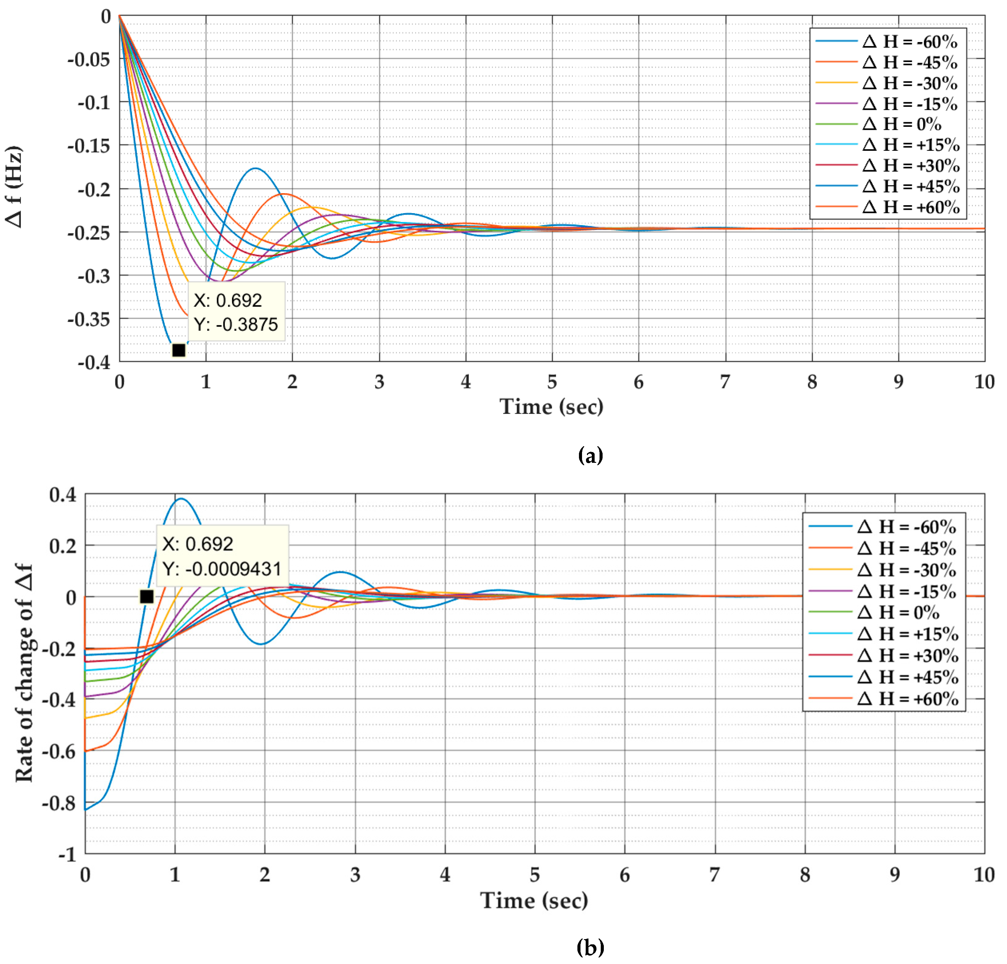
• In a stable power system with only primary control, the level of frequency deviation changes with $\Delta H$, as shown in Figure 4a. For the same load disturbance, the maximum frequency deviation is different from the one calculated using a fixed value of $H$ (i.e., the case when $\Delta H=0$).
• The observation presented in the preceding point has significant implications over the conventional model, which does not consider the effect of changes in H over the frequency deviation. From Figure 4a, it is evident that the error in calculation of the amount of frequency deviation could be as high as 43% for the extreme cases (i.e., $\Delta H=+60\% \mathrm{and} \Delta H=-60\%$) and 30% for $\Delta H=0\% \mathrm{and} \Delta H=-60\%.$It is notable that, from a practical perspective, only a major portion of ESS devices can introduce such a significant difference. However, the results presented in Figure 4a indicate the importance of considering variation in the inertia constant.
• Additionally, the observation presented in the previous points has practical applications as well. For example, the capacity determination of spinning/nonspinning reserves is also dependent on the calculated frequency deviation; therefore, an error in the $H$ estimation can lead to over/undercapacity reserves. Similarly, the reliability of frequency relays is also jeopardized if $H$ is miscalculated or there are changes in its value due to the virtual inertia provided by ESS. It is once again iterated that, in conventional LFC models, the value of $H$ is considered to be constant and does not change during an operational time-period.
• The rate of change of the frequency deviation in Figure 4b is zero when the frequency deviation in Figure 4a touches a maximum or minimum point. As discussed earlier, the first zero-crossing of $\partial \Delta f(t)/\partial t$ corresponds to $\Delta f_{\max }(t)$ in a stable power system. This is demonstrated for a simulation run with $\Delta H=-60\%$. The maximum frequency deviation occurs at $t=0.692 \mathrm{s}$, as verified by the curve shown in Figure 4b. For the sake of clarity, this observation is highlighted for only one case, although it is valid for all simulation cases.

4.2. Case II: An Unstable Power System with Primary Control

The effects of changes in $H$ on the PSFR for an unstable power system primary control only are shown in Figure 5. Since the power system is not stable, therefore, the load disturbance takes the frequency deviation to higher levels. The instability is modeled by converting the left-half plane pole of the turbine TF to a pole in the right-half plane (i.e., $T_{tur}=1/(-s{T}_t+1)$). Further, the generation rate constraint (GRC) of 10% does not allow extreme changes to the power, though the frequency response remains unstable. The key points of this simulation study are presented as follows:

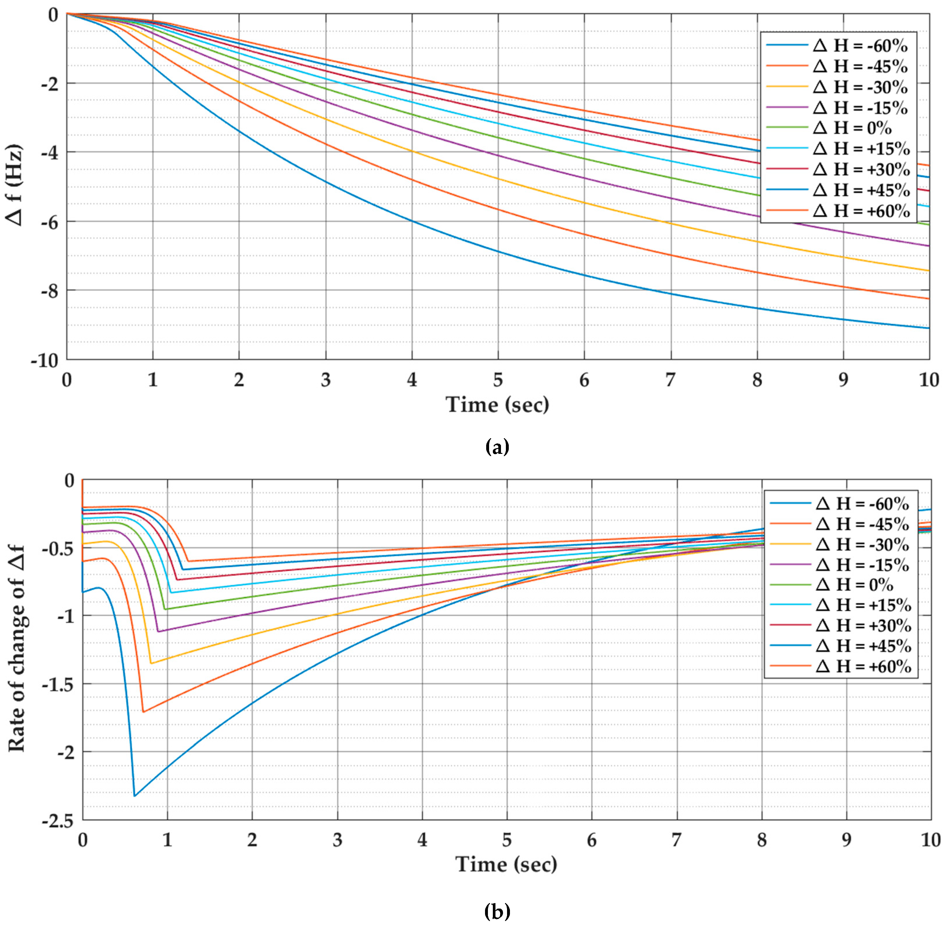
• Although the frequency response is unstable in all cases, however, the level of the frequency deviation changes with $\Delta H$, as shown in Figure 5a. In some cases, the response of the frequency deviation is quicker than the other cases.
• The observation presented in the preceding point also has practical considerations. For example, the frequency relays can mal-operate if $H$ is miscalculated or there are changes in its value due to the virtual inertia provided by ESS.
• As the frequency deviation goes much beyond the operational limits, the shown simulation time of $10\mathrm{s}$ in this study provides enough information. Since the power system is unstable, the frequency deviation should (theoretically) keep on increasing, and its time derivative will not be zero. In any case, the practical power plants have control, and protective devices (e.g., frequency relays or generation rate limiters) that do not allow their operation after certain limits on $\Delta f(t)$ and $\partial \Delta f(t)/\partial t$ are met.

4.3. Case III: A Stable Power System with Primary and Supplementary Controls

Figure 6 shows the effects of variation in $H$ on the PSFR for a stable power with primary and supplementary controls. Again, the changes in $H$ are made with a step of 15%. In contrast to previous cases, the power system has an integral control action; therefore, the frequency deviation goes to zero, as shown in Figure 6a. The summary of observations for this simulation study is presented as follows:

• For the same load disturbance, the level of frequency deviation changes with $\Delta H$. As shown in Figure 6a, $\Delta f_{\max }(t)$ and $t_{\max }$ are different for all cases. This observation calls for the need of accurate information about the power system’s inertia constant. It is notable that, as long as the power system reserves have enough capacity, the stability of a power system is not jeopardized. In any case, a significant difference in the actual and calculated value of $H$ may result in insensitive or oversensitive behavior of the protective relays. It is once again explained that a huge amount of ESS can introduce such a significant difference.
• Whenever $\Delta f(t)$ reaches a maximum or minimum point, $\partial \Delta f(t)/\partial t=0$, as shown in Figure 6b. As discussed earlier, the first zero crossing of $\partial \Delta f(t)/\partial t$ corresponds to $\Delta f_{\max }(t)$ in a stable power system. This is demonstrated for a simulation run with $\Delta H=-60\%$. The maximum frequency deviation occurs at $t=0.66 \mathrm{s},$ as verified by the curve shown in Figure 6b. For the sake of clarity, this observation is highlighted for only one case, although it is valid for all simulation cases.

4.4. Case IV: An Unstable Power System with Primary and Supplementary Controls

The effects of changes in $H$ on the PSFR for an unstable power system with primary and supplementary controls are shown in Figure 7. The instability is modeled by converting the left-half plane pole of the turbine TF to a pole in the right-half plane, as explained earlier. Since the power system is not stable, therefore, the load disturbance keeps on increasing the frequency deviation. The following points summarize the important observations of this simulation study:

• Although the frequency response is unstable in all cases, however, the level of the frequency deviation changes with$\Delta H$, as shown in Figure 7a. In some cases, the response of the frequency deviation is quicker than the other cases. In other words, the frequency relays can trip earlier or later than expected if there is a difference between the actual and calculated $H$.
• As shown in Figure 7b, the rate of change in the frequency deviation will not go to zero for an unstable power system. This is due to the existence of a right-half plane pole in the system TF, which makes the error grow. It is once again explained that, due to the deployment of the GRC, the response does not shoot instantaneously. The results shown in Figure 7 are for a demonstrative purpose to show the significance of an accurate calculation of $H$ for an improved PSFR. Further, the practical systems do have watchful protection that does not allow the generator to operate beyond set limits [6].

5. Conclusions

The modern power systems have increased the role of ESS, which can provide VI with the help of power electronics-based power converters. These sources of VI are seen as an alternative of the synchronous generator in the context of the power grid’s stability enhancements. There exist several simulation studies that show the promising role of VI in frequency profile improvements of power systems using the well-established LFC model. These studies, however, do not consider the changes in the inertia coefficient due to significant penetration of ESS. This work, on the other hand, provides a modified LFC model which includes the role of increased VI. The sensitivity function derived in this work shows the importance of the inertia coefficient in the LFC model. The stability analysis and simulation results show that the effects of differences in the calculated and actual value of $H$ could be detrimental, as it can result in the mal-operation of frequency relays or improper calculations of power reserves. The findings of this study call for the proper modeling of ESS for VI and an accurate and dynamic calculation method of the inertia coefficient of the power system.

As a future work, experimentation of the proposed model in a hardware-in-the-loop configuration could lead to interesting results. Moreover, the presented work can be extended by taking into account the nonlinearities of the power system and considering complex multi-machine, multi-area configurations. Additionally, the presented model can be augmented with consideration of changes in the damping coefficient of the power system.

References

- Anderson, P.M.F. Power System Control and Stability; John Wiley & Sons: Hoboken, NJ, USA, 2008. [Google Scholar]
- Machowski, J.; Bialek, J.W.; Bumby, J. Power System Dynamics: Stability and Control; John Wiley & Sons: Hoboken, NJ, USA, 2011. [Google Scholar]
- Amraee, T.; Darebaghi, M.G.; Soroudi, A.; Keane, A. Probabilistic under frequency load shedding considering RoCoF relays of distributed generators. IEEE Trans. Power Syst. 2018, 33, 3587–3598. [Google Scholar] [CrossRef]
- Wang, L.; Sun, W.; Zhao, J.; Liu, D. A Speed-Governing System Model with Over-Frequency Protection for Nuclear Power Generating Units. Energies 2019, 13, 137. [Google Scholar] [CrossRef]
- Jia, J.; Yang, G.; Nielsen, A.H.; Rønne-Hansen, P. Hardware-in-the-loop Tests on Reverse Power and Over-Frequency Protection for Synchronous Condensers. In Proceedings of the Cigre Aalborg 2019: International Symposium, Aalborg, Denmark, 4–7 June 2019; p. 104. [Google Scholar]
- Power Systems Relaying Committee. IEEE Guide for the Application of Protective Relays Used for Abnormal Frequency Load Shedding and Restoration. IEEE Std C 2007, 37, 1–55. [Google Scholar]
- Bevrani, H. Robust Power System Frequency Control; Springer International Publishing: Cham, Switzerland, 2014. [Google Scholar]
- Zhong, Q.; Weiss, G. Synchronverters: Inverters That Mimic Synchronous Generators. IEEE Trans. Ind. Electron. 2011, 58, 1259–1267. [Google Scholar] [CrossRef]
- Tamrakar, U.; Shrestha, D.; Maharjan, M.; Bhattarai, P.B.; Hansen, M.T.; Tonkoski, R. Virtual Inertia: Current Trends and Future Directions. Appl. Sci. 2017, 7, 654. [Google Scholar] [CrossRef]
- Cleary, B.; Duffy, A.; Bach, B.; Vitina, A.; O’Connor, A.; Conlon, M. Estimating the electricity prices, generation costs and CO2 emissions of large scale wind energy exports from Ireland to Great Britain. Energy Policy 2016, 91, 38–48. [Google Scholar] [CrossRef]
- Smith, R. UK Future Energy Scenarios. In National Grid2014; NRC: Warwick, UK, 2013. [Google Scholar]
- Albu, M.; Calin, M.; Federenciuc, D.; Diaz, J. The measurement layer of the Virtual Synchronous Generator operation in the field test. In Proceedings of the 2011 IEEE International Workshop on Applied Measurements for Power Systems (AMPS), Aachen, Germany, 28–30 September 2011; pp. 85–89. [Google Scholar]
- Karapanos, V.; Haan, S.W.H.; Zwetsloot, K. Testing a Virtual Synchronous Generator in a Real Time Simulated Power System. In Proceedings of the International Conference on Power Systems Transients (IPST2011), Delft, The Netherlands, 14–17 June 2011. [Google Scholar]
- Van, T.V.; Visscher, K.; Diaz, J.; Karapanos, V.; Woyte, A.; Albu, M.; Bozelie, J.; Loix, T.; Federenciuc, D. Virtual synchronous generator: An element of future grids. In Proceedings of the 2010 IEEE PES Innovative Smart Grid Technologies Conference Europe (ISGT Europe), Gothenberg, Sweden, 11–13 October 2010; pp. 1–7. [Google Scholar]
- Zaman, M.S.U.; Bukhari, S.B.A.; Haider, R.; Khan, M.O.; Kim, C.H. Effects of Modified Inertia Constant and Damping Coefficient on Power System Frequency Response. Int. J. Renew. Energy Res. (IJRER) 2019, 9, 525–531. [Google Scholar]
- Ma, Y.; Cao, W.; Yang, L.; Wang, F.; Tolbert, L.M. Virtual Synchronous Generator Control of Full Converter Wind Turbines With Short-Term Energy Storage. IEEE Trans. Ind. Electron. 2017, 64, 8821–8831. [Google Scholar] [CrossRef]
- Saeed Uz Zaman, M.; Bukhari, B.S.; Hazazi, M.K.; Haider, M.Z.; Haider, R.; Kim, C.-H. Frequency Response Analysis of a Single-Area Power System with a Modified LFC Model Considering Demand Response and Virtual Inertia. Energies 2018, 11, 787. [Google Scholar] [CrossRef]
- Kerdphol, T.; Rahman, S.F.; Mitani, Y.; Hongesombut, K.; Küfeoğlu, S. Virtual Inertia Control-Based Model Predictive Control for Microgrid Frequency Stabilization Considering High Renewable Energy Integration. Sustainability 2017, 9, 773. [Google Scholar] [CrossRef]
- Hirase, Y.; Abe, K.; Sugimoto, K.; Sakimoto, K.; Bevrani, H.; Ise, T. A novel control approach for virtual synchronous generators to suppress frequency and voltage fluctuations in microgrids. Appl. Energy 2018, 210, 699–710. [Google Scholar] [CrossRef]
- Li, C.; Xu, J.; Zhao, C. A Coherency-Based Equivalence Method for MMC Inverters Using Virtual Synchronous Generator Control. IEEE Trans. Power Deliv. 2016, 31, 1369–1378. [Google Scholar] [CrossRef]
- Bevrani, H.; Raisch, J. On virtual inertia application in power grid frequency control. Energy Procedia 2017, 141, 681–688. [Google Scholar] [CrossRef]
- Saeed Uz Zaman, M.; Haider, R.; Bukhari, S.B.A.; Ashraf, H.M.; Kim, C.-H. Impacts of Responsive Loads and Energy Storage System on Frequency Response of a Multi-Machine Power System. Machines 2019, 7, 34. [Google Scholar] [CrossRef]
- Huang, H.; Li, F. Sensitivity analysis of load-damping characteristic in power system frequency regulation. IEEE Trans. Power Syst. 2012, 28, 1324–1335. [Google Scholar] [CrossRef]
- Pradhan, C.; Bhende, C.N. Frequency sensitivity analysis of load damping coefficient in wind farm-integrated power system. IEEE Trans. Power Syst. 2016, 32, 1016–1029. [Google Scholar]
- Huang, H.; Li, F. Sensitivity analysis of load-damping, generator inertia and governor speed characteristics in hydraulic power system frequency regulation. In Proceedings of the 2014 Australasian Universities power engineering conference (AUPEC), Perth, Australia, 28 September–1 October 2014; pp. 1–6. [Google Scholar]
- Nguyen, N.T.; Le, D.D.; Moshi, G.G.; Bovo, C.; Berizzi, A. Sensitivity analysis on locations of energy storage in power systems with wind integration. IEEE Trans. Ind. Appl. 2016, 52, 5185–5193. [Google Scholar] [CrossRef]
- Zaman, M.S.U.; Bukhari, S.B.A.; Haider, R.; Khan, M.O.; Baloch, S.; Kim, C.-H. Sensitivity and stability analysis of power system frequency response considering demand response and virtual inertia. IET Gener. Transm. Distrib. 2019. [Google Scholar] [CrossRef]
- Wang, X.; Yue, M.; Muljadi, E. PV generation enhancement with a virtual inertia emulator to provide inertial response to the grid. In Proceedings of the 2014 IEEE Energy Conversion Congress and Exposition (ECCE), Pittsburgh, PA, USA, 14–18 September 2014; pp. 17–23. [Google Scholar]
- Hosseinipour, A.; Hojabri, H. Virtual inertia control of PV systems for dynamic performance and damping enhancement of DC microgrids with constant power loads. IET Renew. Power Gener. 2017, 12, 430–438. [Google Scholar] [CrossRef]
- Tielens, P.; Van Hertem, D. The relevance of inertia in power systems. Renew. Sustain. Energy Rev. 2016, 55, 999–1009. [Google Scholar] [CrossRef]
- Arani, M.F.M.; El-Saadany, E.F. Implementing virtual inertia in DFIG-based wind power generation. IEEE Trans. Power Syst. 2012, 28, 1373–1384. [Google Scholar] [CrossRef]
- Sondhi, S.; Hote, Y.V. Fractional order PID controller for load frequency control. Energy Convers. Manag. 2014, 85, 343–353. [Google Scholar] [CrossRef]
- Anderson, P.M.; Mirheydar, M. A low-order system frequency response model. IEEE Trans. Power Syst. 1990, 5, 720–729. [Google Scholar] [CrossRef]
- Saadat, H. Power System Analysis; McGraw-Hill: Madison, WI, USA, 1999. [Google Scholar]
- Ogata, K. Modern Control Engineering, 5th ed.; Prentice-Hall: Upper Saddle River, NJ, USA, 2010. [Google Scholar]
- Pourmousavi, S.A.; Nehrir, M.H. Introducing Dynamic Demand Response in the LFC Model. IEEE Trans. Power Syst. 2014, 29, 1562–1572. [Google Scholar] [CrossRef]