Abstract
Formation lithology identification is of great importance for reservoir characterization and petroleum exploration. Previous methods are based on cutting logging and well-logging data and have a significant time lag. In recent years, many machine learning methods have been applied to lithology identification by utilizing well-logging data, which may be affected by drilling fluid. Drilling string vibration data is a high-density ancillary data, and it has the advantages of low-latency, which can be acquired in real-time. Drilling string vibration data is more accessible and available compared to well-logging data in ultra-deep well drilling. Machine learning algorithms enable us to develop new lithology identification models based on these vibration data. In this study, a vibration dataset is used as the signal source, and the original vibration signal is filtered by Butterworth (BHPF). Vibration time–frequency characteristics were extracted into time–frequency images with the application of short-time Fourier transform (STFT). This paper develops lithology classification models using new data sources based on a convolutional neural network (CNN) combined with Mobilenet and ResNet. This model is used for complex formation lithology, including fine gravel sandstone, fine sandstone, and mudstone. This study also carries out related model accuracy verification and model prediction results interpretation. In order to improve the trustworthiness of decision-making results, the gradient-weighted class-activated thermal localization map is applied to interpret the results of the model. The final verification test shows that the single-sample decision time of the model is 10 ms, the test macro precision rate is 90.0%, and the macro recall rate is 89.3%. The lithology identification model based on vibration data is more efficient and accessible than others. In conclusion, the CNN model using drill string vibration supplies a superior method of lithology identification. This study provides low-latency lithology classification methods to ensure safe and fast drilling.
1. Introduction
Lithology classification of underground formation is of great importance in the field of oil and gas exploration engineering as lithology represents the reservoir petrophysical characteristics [1]. There are two traditional data resources for classifying the lithofacies. They are underground core (cuttings) observation and well-logging data analysis [2,3,4,5]. Vibration data of drill string can also be used to make real-time lithology identification considering different formation characteristics [6,7].
Computer capabilities enable geologists to make lithology predictions more intelligently. More efforts for lithology identification are carried out with well-logging data by different machine learning methods, including Artificial Neural Network (ANN), Support Vector Machine (SVM), Random Forest (RF), Gradient Boosted Decision Tree (GBDT) [6,7,8,9,10].
Some researchers made lithology prediction based on logging data by using artificial neural networks [11,12,13]. It is demonstrated that lithofacies information from images could be used for lithology identification based on ANN [14]. Tom Horrocks used wire logs to study lithology classification based on three machine learning methods, including Naïve Bayes classifier (NB), SVM, and ANN. And committee and singular architectures are studied in the three machine learning methods [9]. Xie made an evaluation of five machine learning algorithms, including NB, SVM, ANN, RF, and Gradient Tree Boosting (GTB) in lithology classification using well-logging data. RF and GTB showed more advantages on identification accuracy than others [10]. Ren applied ANN with a probabilistic statistical method to make lithology identification. ANN, in this study, showed better accuracy over other algorithms [15].
SVM (Support Vector Machine) classifier is a popular machine learning method in the application of sedimentary rock lithology identification. SVM can be used in drilling and laboratory petrophysical analysis of lithofacies [4,5,9,10,16,17,18].
Random Forest is always applied to make underground formation lithology compared with other machine learning algorithms, such as GTB, GBM, and AdaBoost [8,10,19].
Wang applied an optimized K-Nearest Neighbors clustering to make efficient lithology classification based on weighted cosine distance. And the optimized KNN displayed accurate rates on sandstone recognition [20].
Wood used an optimized-nearest neighbor method to make lithofacies and stratigraphy identification. And the prediction in his study showed advantages over the regression-based and neural-network-based prediction [21].
Dev and Eden focused on GBDT systems, including XGBoost, LightGBM, and CatBoost. LightGBM and CatBoost showed better performances on lithology classification by utilizing well-logging data through some parameter evaluations (Pr, Re, and F1-score) [8].
Khasanov made some investigations on color distribution analysis of lithology classification. Baraboshkin applied convolutional neural networks on rock characterization based on color distribution and feature extraction by using different neural network architectures. GoogleNet has a better performance than other algorithms [22].
Hall used an approach to make a lithofacies classification based on borehole image logs and core photos [23]. Many studies of lithology identification are based on borehole image logs [24,25,26]. Valentín proposed a methodology for lithology identification based on a deep residual convolutional neural network with the application of borehole images [27].
Imamverdiyev applied a new 1D-convolutional neural network (CNN) model by using the logging data as the input dataset in lithology identification. Then it is compared with four machine learning methods, and it shows a better performance in prediction than other methods [28]. It is a good deep learning model in lithology classification until now and shows its excellent performance. This study mainly uses logging data after drilling.
The research in this paper uses vibration data so that real-time prediction could be received in the drilling process. Drill string vibrations are inevitable during the drilling process, and they are recorded in three directions. Vibrations are measured by accelerometers near the drill bit. They can supply the underground formation conditions and rock characteristics [6].
Drill string vibration datasets are always utilized to improve drilling performance [29,30]. It can be applied to reduce friction and enhance the rate of penetration [31]. And drill string vibration is of great importance that many studies are about the analysis of downhole vibration. The downhole vibration data is also easier to access than well-logging and cutting logging data [32,33].
Drill string vibrations are unavoidable and can lead to negative effects on drilling performance by damaging the drill strings. However, it is also of great importance for drilling process optimization.
In 2012, AlexNet won the ImageNet large-scale visual recognition challenge with a high prediction accuracy rate of 10.8%. The important result of this paper is that the deep convolutional neural network can effectively implement image recognition and classification tasks [34].
In this paper, drill string vibrations are applied to make lithology identification through a convolutional neural network algorithm. It can help to make real-time drilling parameter modifications in the drilling process.
Most of the previous lithology classification investigations are based on well-logging datasets. The previous models cannot make the same real-time performance as the novel method in this paper. In this study, drill string datasets are applied to achieve a novel real-time lithology identification model through a convolutional neural network algorithm. We carried out the following work.
Firstly, drill string vibration datasets are the data sources, and time–frequency images are obtained based on vibration characteristics. Secondly, a formation lithology identification model is built based on a convolutional neural network for three kinds of rock by utilizing time–frequency images, which combine the advantages of Mobilenet and ResNet. Lastly, the model prediction result explanation is applied to the formation lithology identification model by a class-activated thermal map. The results showed that the decision time is 10 ms, and the model takes up 49.38 KB storage space. It helps to achieve a real-time lithology identification model. Traditional lithology identification models based on well-logging data have some disadvantages, such as data acquisition lag, complex feature extraction, and limited interpretation. Therefore, the formation of a lithology identification model based on a convolutional neural network using drill string vibration data is a novel method for lithofacies prediction.
2. Drill String Vibration Data Processing
In order to obtain the best generalization performance models, data samples need to cover the sample space for lithology identification. Improving the signal-to-noise ratio of vibration signals helps the datasets to perform lithology identification discrimination more accurately.
2.1. Drill String Vibration Data Sampling
During the sample selection process, we need to consider the sample numbers, sample frequency, and sample lithology. Vibration datasets in this study are from drill string data of an ultra-deep well in Kuqa, which is located in west China. The data depth is 5000~6000 m. Previous researches showed that high and low frequency data generated by downhole drilling string vibration represent different physical meanings. The lower frequency band reflects the working status of the drilling tool, and a higher frequency band reflects the lithological characteristics [35]. Sample frequency is set to 20 Hz, and the collected lithology is fine gravel sandstone, fine sandstone, and mudstone.
By using the vibration sensors, real-time vibration data could be recorded, including axial vibrations, torsional vibrations, and lateral vibrations. And they are recorded according to the directions X, Y, and Z [35].
2.2. Vibration Data Processing
Butterworth High Pass Filter (BHPF) is used for data cleansing in this study. BHPF frequency band transition is smooth, and the attenuation is slow. After Fourier transform, time-domain data is converted into frequency-domain data, and typical spectrum diagrams of three lithologies are observed. Based on the extraction of one-dimensional features of lithology on time and frequency images, short-time Fourier transform (STFT) is used to select time–frequency characteristics changes to form a time–frequency image of the vibration signal.
2.2.1. Time-Domain Characteristics of Different Lithological Vibration Signals
In Figure 1, the time-domain waveform oscillations of fine gravel sandstone in the X and Y directions are the most obvious ones, and the amplitude reflects the difference, indicating that the gravel particles are contained in the stratum. Compared with the fine gravel sandstone, the time-domain waveform oscillations of fine sandstone in the X and Y directions are weaker, indicating that the fine sandstone particles are relatively small and the homogeneity of fine sandstone is relatively good. The time-domain waveform oscillations of mudstone in the X and Y directions are small, and the waveform does not change very much.
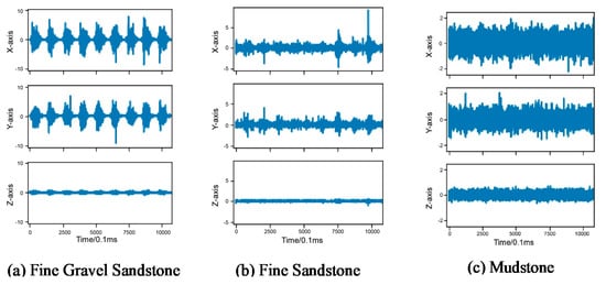
Figure 1.
Typical time-domain diagram of three different lithologies.
Vibration signals of downhole tools are collected, and the time-domain characteristics of the drill string vibration data are analyzed. In Figure 1, X is one of the directions in vibration logging data, so are Y and Z. Mean is the average value of each direction, and rms is short for root mean square. Peak represents the peak data of the drilling string vibration in different directions. R is square root amplitude, lp is peak indicator, and Cf is pulse indicator. The Fourier transform of the stationary signal frequency is used to analyze the frequency domain characteristics. Dimensionless indicators, such as the peak indicator and the pulse indicator, represent the shock characteristics of the vibration signal. They are descriptive statistics in the time-domain of vibration, and they are helpful for studying vibration data characteristics.
In Figure 2, the mean value, root mean square, and peak value of fine sandstone and mudstone range from 0 to 5. The mean value and root mean square value of gravelly fine sandstone range from 0 to 5, and the peak value of it is slightly greater than 5. The peak and pulse indicators of the fine gravel sandstone in the X and Y directions are higher than those of the other two types of lithology, showing more obvious impact characteristics, which may be due to the sudden increase in load caused by encountering high-strength particles. Peak and pulse indicators of the fine gravel sandstone in the Z direction are lower than those of the other two types of lithology.
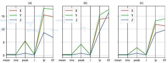
Figure 2.
Comparison of characteristic variables of vibration in the time-domain. (a) Fine Gravel, Sandstone, (b) Fine Sandstone, (c) Mudstone.
2.2.2. Frequency Domain Characteristics of Different Lithological Vibration Signals
Representing a discrete sequence as a series of complex exponential functions can be used to obtain the frequency diagram of the time-domain vibration signal. In Figure 3, the frequency diagram shows the component strength of the original signal at each frequency and the characteristic frequency of the signal. The spectral intensity of fine gravel sandstone has obvious characteristic peaks in the Z direction. The corresponding working condition is that when the high-intensity conglomerate particles are encountered, the frequency spectrum jitters. The homogeneity of fine sandstone and mudstone is slightly better, and the frequency characteristics are similar, but the intensity and coverage frequency of each vibration direction are different. The smaller amplitude of mudstone frequency indicates lower mudstone strength. There are many unpredictable samples in fine sandstone and mudstone, which can be used as the optimization and promotion of the lithology identification model.
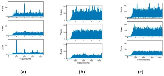
Figure 3.
Typical frequency diagram of three different lithologies. (a) Fine Gravel Sandstone, (b) Fine Sandstone, (c) Mudstone.
Through the Fourier transform processing of the initial time-domain vibration signal of the tool, the spectrum intensities of the three lithologies along the vibration direction are obtained in Figure 4, and the spectrum intensities corresponding to the lithology and the vibration direction are counted to obtain the mean distribution. By statistically comparing the average distribution of the spectral intensity of three lithologies in three vibration directions, it is found that the peaks of the spectral intensity of the three lithologies in the Z direction are higher than those in the other two directions. The peaks of the spectral intensity of the fine gravel sandstones in the X direction are larger. The peaks of the fine gravel sandstones are slightly higher than those of the fine sandstones.
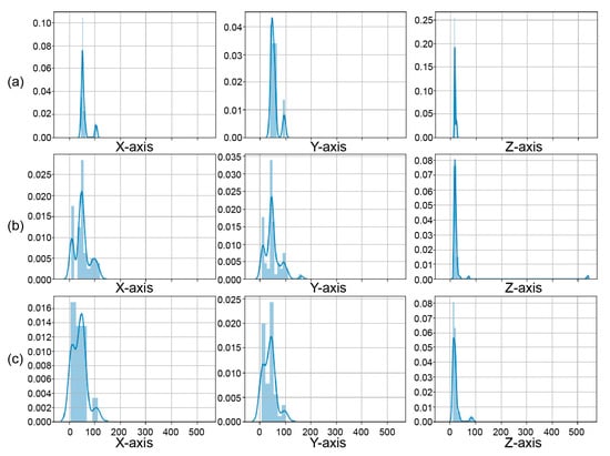
Figure 4.
Histogram of mean spectral intensity of three lithological samples. (a) Fine Gravel Sandstone, (b) Fine Sandstone, (c) Mudstone.
2.2.3. Time–frequency Characteristics of Different Lithological Vibration Data
Frequency domain processing, also known as spectrum analysis, is a time–frequency transform based on the Fourier transform. The result obtained is a function of frequency, called the spectral function. The real and imaginary parts of the result of the Fourier transform can be converted into the amplitude spectrum and the phase spectrum.
Short-Time Fourier Transform and Wavelet Transform Calculation Principles
(a) Short-time Fourier transform
The underground drill string vibration data is a non-stationary signal with transient characteristics. Short-time Fourier transform has significant advantages in processing non-stationary signals [36]. In Formula (1), it is that the representation information of the short-time Fourier transform contains the time dimension. In this study, the Gabor transform is used for signal processing. The Gabor transform is a short-time Fourier transform that uses a Gaussian function as the window function. The Gaussian function is the window function that can best balance both the time axis and the frequency axis. The Gaussian function is a characteristic function of the Fourier transform, and its properties are unchanged after the transformation. Therefore, after the Gabor transformation, the properties of the time axis and the frequency axis are symmetrical to each other.
where x[n] is the signal to be transformed, w[n − m] is the window function, and m is the signal overlap area.
The horizontal axis of the time–frequency graph represents the time dimension of the signal. The vertical axis represents the change in the frequency dimension of the signal. The color shading represents the intensity of the spectrum under a certain time and frequency limit in Figure 5. In this study, the main frequencies of 500 and 1000 Hz are extracted.
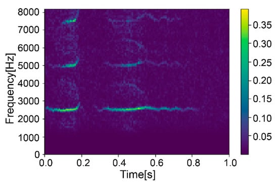
Figure 5.
Time–frequency graph in short-time Fourier transform.
(b) Wavelet transforms
When performing time–frequency analysis, wavelet transform is also a commonly used tool. Compared with short-time Fourier transform, it is characterized by adaptive frequency changes. Therefore, a lower time resolution can be used in the high frequency band to improve the frequency resolution and provide a sufficiently long vibration signal to capture the frequency domain characteristics.
The focus of wavelet analysis is on the selection of “mother wavelet”, which has translation and scaling parameters to match the signal. Its transformation formula is as follows:
where x(t) is the signal to be transformed, a is a scale parameter, b is a translation parameter, and ψ(t) is the wavelet function. Common wavelet functions include Meyer, Morlet, and Mexican hat.
The wavelet transform spectrum with Gaussian wavelet Cgau as the wavelet function in the time–frequency image is given in this paper. (Figure 6) The original vibration signal is disturbed by low-frequency noise, and the wavelet transform can show the change of spectral intensity in low-frequency conditions. Compared with short-time Fourier transform, wavelet transform can improve the time and frequency resolution, but the computation efficiency is low. Compared with the original vibration signal under the same conditions, the computation time is increased by about 10 times, and a suitable mother wavelet signal needs to be screened.
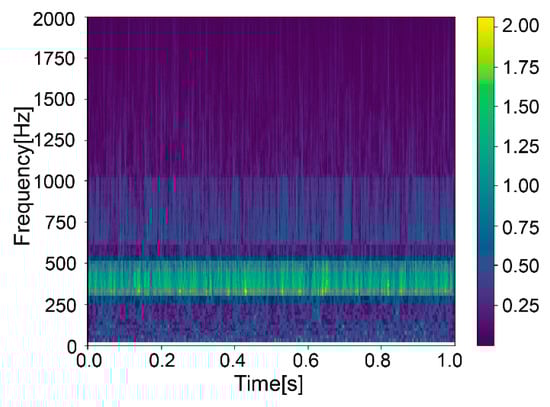
Figure 6.
Time–frequency graph in wavelet transform.
Figure 6 shows the low-frequency noise interference from raw vibration data. The low-frequency time–frequency plot shows changes in spectral intensity at low frequencies. Wavelet transform spectrogram improves time and frequency resolution discrimination. Compared with the original vibration data with the same conditions, the wavelet transform spectrogram has low calculation efficiency, and the calculation time increases by about 10 times.
Time–frequency Image Analysis of Different Lithologies
A time–frequency image of raw vibration data can be obtained by short-time Fourier transform and wavelet transform. A time–frequency image has a high density of information. This unstructured image data is suitable for processing using convolutional neural networks. Time–frequency images of raw vibration data provide training data samples for building complex lithology recognition models.
(a) Short-time Fourier transform time–frequency image features
Short-time Fourier transform transforms the signal into the time–frequency domain. Sliding window intercepts unstable signals, and the signals in the sliding window can be approximated as stable signals. Therefore, the frequency domain of a time-varying signal can be decomposed into a time–frequency domain. Then, the lithology can be classified using the convolutional neural network’s efficient feature extraction and pattern recognition classification capabilities.
Figure 7 is a short-time Fourier transform time–frequency domain image of the first sample of three lithologies. Since the original signal is obtained by a fixed sliding window during the short-time Fourier transform, the time–frequency image is consistent in the resolution of each time-domain and frequency domain. Discrete grids can be seen in the time–frequency images. Comparing Figure 7 with the spectrum diagram in Figure 3, we can find that the time–frequency image shows the frequency intensity along the time axis direction. By observing the color scale, it is found that the three lithological main frequency distributions are different. The time–frequency images of fine sandstone and mudstone along the three directions are similar. It is similar to the regular vibration covering the frequency range. Among them, the fine gravel sandstone has significant frequency changes in the X and Z directions.
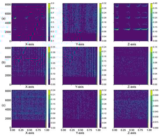
Figure 7.
Time–frequency image after short-time Fourier transform. (a) Fine Gravel Sandstone, (b) Fine Sandstone, (c) Mudstone.
(b) Wavelet transform time–frequency image features
Figure 8 is a wavelet transform time–frequency image of the three lithological samples corresponding to Figure 3. The wavelet transform has the ability to adapt to two dimensions of time and frequency. It improves the frequency domain resolution at high frequencies and the time resolution at low frequencies. Comparing Figure 8 and Figure 3, the wavelet transform can get more local frequency intensity changes. Analysis of wavelet time–frequency images of three lithologies shows that the frequency intensity at 3 KHz is approximately 0. The intensity of the frequency spectrum of fine gravel sandstone vibrating in three directions changes most obviously with time, and the periodic frequency intensity increases in the Z direction. For mudstone, high frequency intensity in the Y direction is more obvious than in the X direction. For fine sandstone, high frequency intensity in the X direction is more obvious than in the Y direction. Fine sandstone and mudstone have almost no change in frequency intensity in the Z direction.
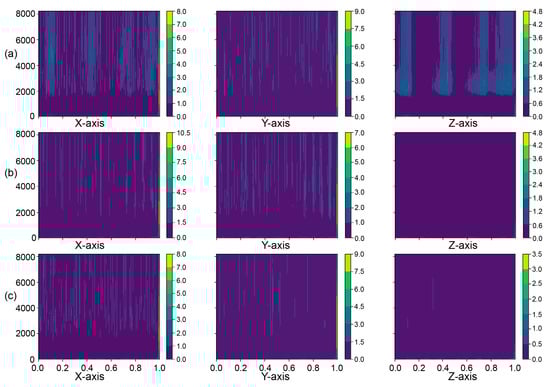
Figure 8.
Time–frequency image after wavelet transform. (a) Fine Gravel Sandstone, (b) Fine Sandstone, (c) Mudstone.
3. Lithology Identification Model Based on Convolutional Neural Network
Convolutional neural network is a feedforward network. Compared with the results of traditional fully connected layer networks, convolution calculations are more suitable for feature extraction of two-dimensional image data. In a deep convolutional neural network, the edge, texture, color, and abstract semantic features of the image are extracted layer by layer using the convolutional network, and then the fully connected layer is used as a classifier to classify the class space.
The convolutional network feature update calculation formula is shown below
where Mj is the set of elements that this layer needs to map; Fj l is the eigenvalue of the position j of the l th layer; kij l is the weight of the convolution kernel at the l th position ij; ∗ is convolution calculation, and it can be analogized to the weighted summation of the eigenvalues in the range of the mapping set. bj l is the extra bias added by position j at level l th layer.
3.1. Lithology Identification Model Establishment Process and Framework
Figure 9 shows the lithology identification model establishment process. The lithology recognition model is implemented based on convolutional layers to extract time–frequency image features. Then the fully connected layer is used for lithology classification. Some special jump connections and convolution kernel combinations are used between the layers to make the model training converge better. Generally, these special connections and combinations form a basic unit, and the model construction can also be expanded based on the basic unit.
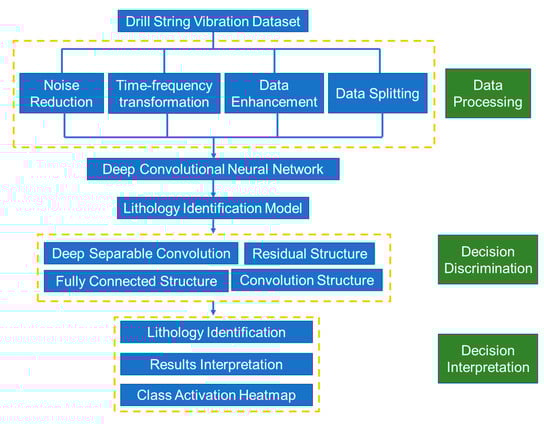
Figure 9.
Lithology identification model establishment process.
The basic calculation process of the lithology identification model includes data processing, data enhancement, model construction initialization, model training, model evaluation, and model tuning. Data processing and data enhancement determine the upper limit of the model’s predictive ability. Model construction, training, and tuning determine whether the model can approach the upper limit.
3.2. Model Architectures and Calculation Process
In view of training efficiency and model complexity, two structural units, MobileNet and ResNet, are generally used to ensure the calculation efficiency and prediction accuracy of the lithology identification model.
MobileNet is mainly composed of deeply separable convolutions. Under the limitations of computation efficiency and computing resources of mobile or embedded devices, it guarantees efficient computing, and at the same time compresses the number of parameters to ensure computing storage efficiency.
ResNet is mainly composed of residual structure, which can effectively control model parameters and maintain the expressiveness of feature transfer. This is helpful to ensure the effectiveness of gradient direction propagation and can build deep networks with rich semantic space.
In addition, we need to use the softmax activation function to normalize and scale the final prediction probability.
MobileNet is a lightweight grid that can effectively reduce the storage and calculation overhead of model networks and provides an effective solution for convolution calculations and parameter storage overhead. The core is to split the traditional convolution process into Depthwise and Pointwise processes, also known as deep separable convolutions.
Comparing traditional convolution (a) and depth separable convolution (b) in Formula (4), the difference between the two calculations is mainly focused on the channel processing of the input data by the convolution check [37].
where m is the number of input layer channels, n is the number of output layer channels, K is the convolution kernel, F is the feature layer, and G is the output feature layer.
ResNet helps suppress performance degradation caused by neural network stacking.
Increasing the depth of the neural network can improve the expression ability of the neural network, but it also increases the risk of gradient disappearance, which leads to the degradation of the performance of the neural network. Therefore, the residual structure helps to solve the model degradation problem of the deep network. The residual unit has the following unit mapping relationship [38].
where Yl is the output of the l th residual unit, Xl is the input of the l th residual unit, F is the residual structure map, Wl is the l th residual structure weight.
The implementation structure of the residual unit is mentioned in He’s study [38]., the residual unit has the identity map x of the upper layer as information to supplement the output unit F(x) of the lower layer, so the training center of gravity of the next stacked residual unit can be transferred to the residual F(x) between y and x.
3.3. Model Network Configuration
The MXNET Deep Learning Framework is applied in this investigation [39]. A network of subject lithological feature extraction and classification is established. MobileNet and ResNet structures are used in the network to ensure that the depth of the network is increased while the model storage calculation overhead is reduced. Specific network parameters are shown in Table 1.

Table 1.
Configuration of network.
In Table 1, the lithology identification model has a total of 16 layers of network stacks and a total of 6859 parameters. The storage space occupied by this model is only 49.38 KB. In the above configuration, the Mobilenet prefix indicates the Mobilenet convolution layer, and the conv prefix indicates the commonly used convolution layer.
The model consists of a 16-layer network stack. The first three layers are a Mobilenet layer structure. The ResNet jump connection structure is embedded in the network. The last six layers are conventional convolution and fully connected layer structures. The number of fully connected neuron nodes is three, which represents the output dimension of three, which is used to distinguish three lithologies. After activation by the softmax function, the highest probability value is selected as the final predicted lithology.
3.4. Lithology Identification Model Training
The data set is split into a training set, a test set, and a validation set. The training set is used to update the iteration parameters for the training process of the lithology classification model. The test set is used to check whether the model has the generalization ability. The validation set is used to monitor the training process. Whether the model accuracy and loss meet the requirements.
The rock recognition model uses the back-propagation algorithm to achieve the training purpose. The parameters are mainly updated by obtaining the partial derivatives of the loss function for each weight parameter. The training process needs to set the hyper-parameters, such as the learning rate, learning decay rate, sample batch processing capacity, and sample iteration rounds. The setting of hyperparameters is related to the model’s convergence rate and final effect. It can add monitoring to the model training process, record weights, gradient changes, and track and observe the model training process to lay the foundation for model tuning.
In addition, in order to further improve the generalization ability of the model, necessary data enhancement measures can be taken on the data, that is, a slight disturbance is applied under the condition that the original data semantics and labels are unchanged. The disturbance can include random cropping, center cropping, image flipping, saturation degree disturbance, and brightness disturbance.
Therefore, the training process of the lithology recognition model needs to consider the data quantity and quality, tuning of hyperparameter settings, network structure design, and training strategies.
When training the lithology recognition model, there are two ways of data and weight flow. One is forward propagation. The data is extracted from the network topic and the prediction results are given. The other is back propagation. The partial derivatives further update the parameter weights, and the training is stopped when the model’s convergence loss function reaches the accuracy requirement or iterative rounds are reached. The complete training process is shown in Figure 10.
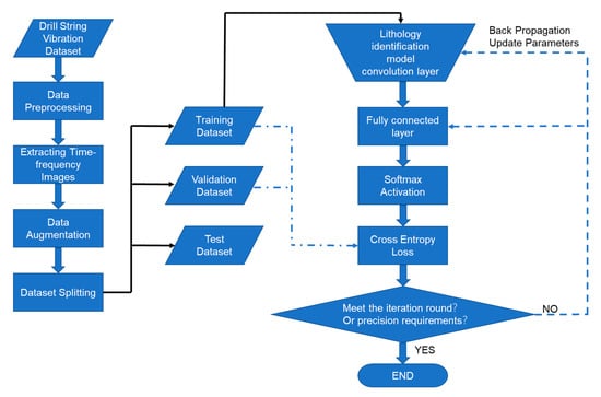
Figure 10.
Lithology recognition model training flowchart.
The training model needs to complete basic tasks, such as data preprocessing, time–frequency image integration, data enhancement, and data set splitting, to ensure reliable data quality and accurate classification labels. The training set and the validation set are used to test the loss cost function of the model and provide parameter gradients. When the model does not meet the end condition, a second iteration occurs, and the parameters are updated according to the back-propagation algorithm.
The back-propagation algorithm needs to calculate the gradient based on the target cost function. Because lithology recognition tasks can be classified as multi-class target tasks, cross-entropy loss is usually chosen as the target cost function for multi-class problems. The formula is as follows:
where M is the target category; yc is the indicator variable, when the predicted category and label are the same, yc is equal to 1, otherwise it is 0. pc is the prediction sample, the probability of c.
The back-propagation algorithm mainly uses the partial derivative of the loss function on the network weight parameters as the gradient and updates the parameters in the reverse direction of the gradient to reduce the loss parameters. [40] The algorithm is as follows:
where wij is model weight, oi is neuron input, y is actual value, netj is neuron output value of this value, φ is activation function, J is loss function, E is error of loss function calculation, ∂E/∂wi is the gradient of error versus weight, which can be obtained by the chain derivation rule, α is learning rate, and Δwij is the weight update amount.
In order to reasonably train, monitor, and evaluate the lithology recognition model, the data set is split into a training set, a validation set, and a test set, with a data volume ratio of 7:2:1. The classification target of the lithology identification model is to distinguish three types of lithology. Therefore, there are three types of lithology samples in the collected raw data. It is not appropriate to use random sampling to determine the three types of data sets during data set splitting. The results after stratified sampling are shown in Table 2
Table 2.
Split dataset.
Effective data augmentation can increase the number of training samples, increase sample diversity, avoid overfitting, and improve the generalization performance of the model. Common enhancement measures include horizontal image flipping, random interception, size conversion, random rotation, and color dithering.
The lithology identification model data source is a time–frequency image converted from vibration data, which has time and frequency dimension information. It is not suitable to use horizontal flip or random flip. Color dithering can be used to simulate noise disturbances, and random cropping of analog signal acquisition is not complete. The fine sandstone time–frequency image is taken as an example to show the data enhancement effect.
The essence of training a neural network is the process of constantly updating the network weights so that they eventually converge on the training target. Before training, you need to build a network and prepare data. Initially, you need to initialize the network weights. During training, you need to update the weights according to the set sample batches, sample iterations, learning rate, and learning rate decay rate. The hyperparameters are set by referring to the previous hyperparameter setting values, combining the data of lithology classification and task characteristics.
Table 3 is the configuration of hyperparameters. The best hyperparameters are finally determined after parameter optimization in Table 4.
Table 3.
Configuration of hyperparameters.
Table 4.
Finetune of hyperparameters.
4. Lithology Identification Model and Verification
After denoising the original vibration data, we extract the video image, configure the lithology recognition model, and strictly follow the training process and strategy to obtain the final lithology recognition model with loss error convergence. After that, the most critical thing is to test the generalization performance of the model prediction, that is, to use the test samples unrelated to the training samples to detect and evaluate the prediction accuracy of the model. This paper uses class activation graphs to make reasonable decision interpretations of prediction results.
4.1. Lithology Identification Model Verification Results
According to the model in the previous section, the optimal model is adjusted, and the test set samples sampled from the hierarchy in the section are taken as the evaluation data set for the model’s final generalization performance. The precision, recall, macro precision, macro recall, and confusion matrix of the test set is counted in turn [41]. Table 5 is the finetune of hyperparameters.
Table 5.
Finetune of hyperparameters.
The trained lithology recognition model is used to predict the test sample and calculate the normalized confusion matrix between the prediction result and the true label of the sample in Figure 11. The lithology recognition model has a good recognition effect on fine gravel sandstone. The prediction result of fine sandstone is acceptable. And the prediction result of Mudstone is general, which can be effectively improved by supplementing mudstone samples. The fine gravel sandstone prediction results have more obvious vibration changes in the time–frequency images of vibration, and the prediction effect is better.
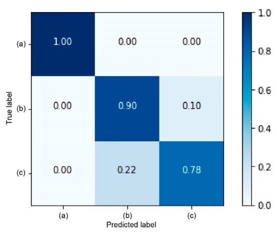
Figure 11.
Normalized confusion matrix of test.
Table 6 shows the precision, recall, macro precision, and macro precision indicators of this test sample set.
Table 6.
Statistical indicators of test dataset.
4.2. Interpretation of Lithology Identification Model Results
According to the final accuracy and recall evaluation indicators, we can see that the lithology identification model has good identification results. The storage space of the model is only 49.38 KB, with a total of 6859 weight parameters. The prediction time of a single sample can be controlled within 10 ms, which achieves the dual advantages of computing efficiency and storage ratio.
Lithology recognition model construction is based on a deep convolutional neural network. The characteristics of deep learning methods have significantly improved the performance of the model. However, the model is not interpretable enough. The reason for the lack of interpretability is that it is difficult to intuitively extract the effective associations and decision linkages between the layers from the huge parameter weights [42].
This paper uses class activation diagrams for model interpretation. Class activation diagrams are used to highlight the decision basis for predicting the interpretation model of relevant regions. In order to explain the decision basis of the lithology identification model, a class activation graph is used to highlight the areas that have a high contribution to the identification result.
The class activation map is a weighted fusion of different channels of the last convolutional layer according to the weighting coefficient to generate a rough thermal positioning map, which is used to highlight the areas in the image that are of high importance to the identification of the prediction target. Gradient coefficient weighted class activation mapping is applied in this study [43].
The gradient-weighted class activation mapping is defined as follows:
where is yc is the score for category c; Ak is the k th channel of the feature map; αkc is the weight of the k th channel category c; Z is the number of pixels in the feature map; (i, j) is the pixel position.
Formula (9) is integrated into the MXNET model through python code (Appendix A), and the recognition results of three lithologies are obtained as shown in the figure below.
From the Grad-CAM submap in Figure 12, the brighter the color of this type of activation heatmap, the stronger the correlation, and the higher the contribution to the prediction of the final target category. Time–frequency images of fine gravel sandstone, fine sandstone, and mudstone will produce different highly correlated thermal localization maps.
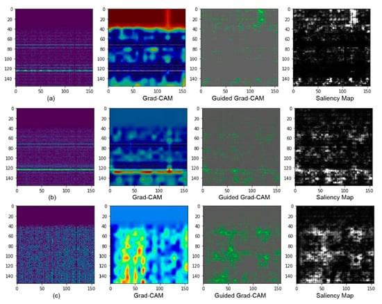
Figure 12.
Class activation diagram for lithology recognition.
5. Conclusions
In this study, a new method of lithology identification relied on drill string vibration data is introduced by utilizing convolutional neural networks. Utilizing the advantages of real-time acquisition of vibration signals and the efficient computation capabilities of deep convolutional networks to process complex unstructured data, a lithology identification model is established to achieve efficient lithology identification analysis. Finally, the decision of the lithology identification model is explained with a class activation diagram judgment basis. The conclusions are as follows:
- (1)
- The vibration data needs to be denoised and high-pass filtered. Due to the low signal-to-noise signal of the drilling tool vibration signal collected in the well, the denoising operation is required, and the lithological characteristics of the rock are mainly concentrated in the high frequency band, so high-pass filtering should be performed.
- (2)
- An end-to-end lithology identification model calculation framework is implemented. The collected vibration data is pre-processed by high-pass filtering and noise reduction, and the short-time Fourier transform is used to extract the time–frequency channel component images of each vibration direction.
- (3)
- A lithology identification model based on the characteristics of the Mobilenet and ResNet structural units is designed and constructed. Finally, the output is classified into three types by using fully connected layers and softmax activation functions, corresponding to three types of target lithology. Designed to have a lithology recognition network with 16 layers of depth, the network has 6859 weight parameters. The storage space occupied by the model is only 49.38 KB, and the time–frequency image inference speed of a single sample can be controlled within 10 ms. The test macro precision rate is 90.0%, and the macro recall rate is 89.3%. Therefore, the model can be adapted to regular embedded or mobile devices.
- (4)
- An explanatory method of the model is provided. The first is a rough positioning heat map that provides a classification basis based on the activation map. Three types of highly correlated time–frequency regions with different lithologies were located using the activation-like thermogram. Fine gravel sandstone has an extremely high frequency region, Mudstone has a stable and continuous main frequency vibration, and Sandstone vibration has a broad but short duration.
Supplementary Materials
Supplementary File 1Author Contributions
Conceptualization, G.C.; Funding acquisition, M.C.; Software, G.H.; Data curation, B.Z.; Validation, Y.G.; Supervision, Y.L.; Writing, G.C. All authors have read and agreed to the published version of the manuscript.
Funding
This study is supported the United Fund Key Program (No. U1762215) and and Chinese National Natural Science Foundation (No. U19B6003-05). This study is also supported the State Key Laboratory of Petroleum Resource and Prospecting, China University of Petroleum, Beijing.
Conflicts of Interest
The authors declare no conflict of interest.
Abbreviations
| ANN | Artificial Neural Network |
| BHPF | Butterworth High Pass Filter |
| GBDT | Gradient Boosted Decision Tree |
| GBM | Gradient Boosting Machines |
| GTB | Gradient Tree Boosting |
| NB | Naïve Bayes classifier |
Appendix A
Grad-CAM code


References
- Buryakovsky, L.; Chilingar, G.; Rieke, H.H.; Shin, S. Fundamentals of the Petrophysics of Oil and Gas Reservoirs; John Wiley & Sons: Hoboken, NJ, USA, 2012; ISBN 1-118-34447-2. [Google Scholar]
- Li, H.; Misra, S. Assessment of miscible light-hydrocarbon-injection recovery efficiency in Bakken shale formation using wireline-log-derived indices. Mar. Pet. Geol. 2018, 89, 585–593. [Google Scholar] [CrossRef]
- Salehi, S.M.; Honarvar, B. Automatic Identification of Formation Iithology from Well Log Data: A Machine Learning Approach. J. Pet. Sci. Res. 2014, 3, 73–82. [Google Scholar] [CrossRef]
- Sun, Z.; Lin, C.; Zhu, P.; Chen, J. Analysis and modeling of fluvial-reservoir petrophysical heterogeneity based on sealed coring wells and their test data, Guantao Formation, Shengli oilfield. J. Pet. Sci. Eng. 2018, 162, 785–800. [Google Scholar] [CrossRef]
- Xiongyan, L.; Jinyu, Z.; Hongqi, L.; ZHANG, S.; Yihan, C. Computational intelligent methods for predicting complex ithologies and multiphase fluids. Pet. Explor. Dev. 2012, 39, 261–267. [Google Scholar]
- Esmaeili, A.; Elahifar, B.; Fruhwirth, R.K.; Thonhauser, G. Experimental Evaluation of Real-Time Mechanical Formation Classification Using Drill String Vibration Measurements. In Proceedings of the SPE Annual Technical Conference and Exhibition, San Antonio, TX, USA, 8–10 October 2012. [Google Scholar]
- Myers, G.; Goldberg, D.; Rector, J. Drill string vibration: A proxy for identifying lithologic boundaries while drilling. In Proceeding of the Ocean Drilling Program Scientific Results (Casey and Miller); Texas A&M University: College Station, TX, USA, 2002; pp. 1–17. [Google Scholar]
- Dev, V.A.; Eden, M.R. Formation lithology classification using scalable gradient boosted decision trees. Comput. Chem. Eng. 2019, 128, 392–404. [Google Scholar] [CrossRef]
- Horrocks, T.; Holden, E.-J.; Wedge, D. Evaluation of automated lithology classification architectures using highly-sampled wireline logs for coal exploration. Comput. Geosci. 2015, 83, 209–218. [Google Scholar] [CrossRef]
- Xie, Y.; Zhu, C.; Zhou, W.; Li, Z.; Liu, X.; Tu, M. Evaluation of machine learning methods for formation lithology identification: A comparison of tuning processes and model performances. J. Pet. Sci. Eng. 2018, 160, 182–193. [Google Scholar] [CrossRef]
- Baldwin, J.L.; Otte, D.N.; Whealtley, C. Computer Emulation of Human Mental Processes: Application of Neural Network Simulators to Problems in Well Log Interpretation. In Proceedings of the SPE Annual Technical Conference and Exhibition, San Antonio, TX, USA, 8–11 October 1989. [Google Scholar]
- Chang, H.-C.; Chen, H.-C.; Kopaska-Merkel, D.C. Identification of Lithofacies Using ART Neural Networks and Group Decision Making. In Proceedings of the Artificial Neural Networks in Engineering Conference, St Louis, MO, USA, 1–4 November 1998; pp. 855–860. [Google Scholar]
- Kohonen, T. Self-organized formation of topologically correct feature maps. Biol. Cybern. 1982, 43, 59–69. [Google Scholar] [CrossRef]
- Ivchenko, A.V.; Baraboshkin, E.E.; Ismailova, L.S.; Orlov, D.M.; Koroteev, D.A.; Baraboshkin, E.Y. Core Photo Lithological Interpretation Based on Computer Analyses. In Proceedings of the IEEE Northwest Russia Conference on Mathematical Methods in Engineering and Technology, Russia, Saint-Petersburg, 10–14 September 2018; pp. 425–428. [Google Scholar]
- Ren, X.; Hou, J.; Song, S.; Liu, Y.; Chen, D.; Wang, X.; Dou, L. Lithology identification using well logs: A method by integrating artificial neural networks and sedimentary patterns. J. Pet. Sci. Eng. 2019, 182, 106336. [Google Scholar] [CrossRef]
- Al-Anazi, A.; Gates, I. A support vector machine algorithm to classify lithofacies and model permeability in heterogeneous reservoirs. Eng. Geol. 2010, 114, 267–277. [Google Scholar] [CrossRef]
- Bérubé, C.L.; Olivo, G.R.; Chouteau, M.; Perrouty, S.; Shamsipour, P.; Enkin, R.J.; Morris, W.A.; Feltrin, L.; Thiémonge, R. Predicting rock type and detecting hydrothermal alteration using machine learning and petrophysical properties of the Canadian Malartic ore and host rocks, Pontiac Subprovince, Québec, Canada. Ore Geol. Rev. 2018, 96, 130–145. [Google Scholar] [CrossRef]
- Sebtosheikh, M.A.; Salehi, A. Lithology prediction by support vector classifiers using inverted seismic attributes data and petrophysical logs as a new approach and investigation of training data set size effect on its performance in a heterogeneous carbonate reservoir. J. Pet. Sci. Eng. 2015, 134, 143–149. [Google Scholar] [CrossRef]
- Sun, J.; Li, Q.; Chen, M.; Ren, L.; Huang, G.; Li, C.; Zhang, Z. Optimization of models for a rapid identification of lithology while drilling-A win-win strategy based on machine learning. J. Pet. Sci. Eng. 2019, 176, 321–341. [Google Scholar] [CrossRef]
- Wang, X.; Yang, S.; Zhao, Y.; Wang, Y. Lithology identification using an optimized KNN clustering method based on entropy-weighed cosine distance in Mesozoic strata of Gaoqing field, Jiyang depression. J. Pet. Sci. Eng. 2018, 166, 157–174. [Google Scholar] [CrossRef]
- Wood, D.A. Lithofacies and stratigraphy prediction methodology exploiting an optimized nearest-neighbour algorithm to mine well-log data. Mar. Pet. Geol. 2019, 110, 347–367. [Google Scholar] [CrossRef]
- Baraboshkin, E.E.; Ismailova, L.S.; Orlov, D.M.; Zhukovskaya, E.A.; Kalmykov, G.A.; Khotylev, O.V.; Baraboshkin, E.Y.; Koroteev, D.A. Deep convolutions for in-depth automated rock typing. Comput. Geosci. 2020, 135, 104330. [Google Scholar] [CrossRef]
- Hall, J.; Ponzi, M.; Gonfalini, M.; Maletti, G. Automatic Extraction and Characterisation of Geological Features and Textures Front Borehole Images and Core Photographs. In Proceedings of the SPWLA 37th Annual Logging Symposium, New Orleans, LA, USA, 16–19 June 1996. [Google Scholar]
- Basu, T.; Dennis, R.; Al-Khobar, B.; Al Awadi, W.; Isby, S.; Vervest, E.; Mukherjee, R. Automated Facies Estimation from Integration of Core, Petrophysical Logs, and Borehole Images. In Proceedings of the AAPG Annual Meeting, Houston, TX, USA, 10–13 March 2002; pp. 1–7. [Google Scholar]
- Chai, H.; Li, N.; Xiao, C.; Liu, X.; Li, D.; Wang, C.; Wu, D. Automatic discrimination of sedimentary facies and lithologies in reef-bank reservoirs using borehole image logs. Appl. Geophys. 2009, 6, 17–29. [Google Scholar] [CrossRef]
- Linek, M.; Jungmann, M.; Berlage, T.; Pechnig, R.; Clauser, C. Rock classification based on resistivity patterns in electrical borehole wall images. J. Geophys. Eng. 2007, 4, 171–183. [Google Scholar] [CrossRef]
- Valentín, M.B.; Bom, C.R.; Coelho, J.M.; Correia, M.D.; Márcio, P.; Marcelo, P.; Faria, E.L. A deep residual convolutional neural network for automatic lithological facies identification in Brazilian pre-salt oilfield wellbore image logs. J. Pet. Sci. Eng. 2019, 179, 474–503. [Google Scholar] [CrossRef]
- Imamverdiyev, Y.; Sukhostat, L. Lithological facies classification using deep convolutional neural network. J. Pet. Sci. Eng. 2019, 174, 216–228. [Google Scholar] [CrossRef]
- Besaisow, A.; Ng, F.; Close, D. Application of ADAMS (Advanced Drillstring Analysis and Measurement System) and Improved Drilling Performance. In Proceedings of the SPE/IADC Drilling Conference, Houston, TX, USA, 27 February–2 March 1990. [Google Scholar]
- Dantas, E.; Cunha, A., Jr.; Soeiro, F.; Cayres, B.; Weber, H. An Inverse Problem via Cross-Entropy Method for Calibration of a Drill String Torsional Dynamic Model. In Proceedings of the 25th ABCM International Congress on Mechanical Engineering (COBEM 2019), Uberlândia, Brazil, 20–25 October 2019. [Google Scholar]
- Esmaeili, A.; Elahifar, B.; Fruhwirth, R.K.; Thonhauser, G. Laboratory Scale Control of Drilling Parameters to Enhance Rate of Penetration and Reduce Drill String Vibration. In Proceedings of the SPE Saudi Arabia Section Technical Symposium and Exhibition, Al-Khobar, Saudi Arabia, 8–11 April 2012. [Google Scholar]
- Chiu, S.K.; Anno, P.D. System and Method for Determining Drill String Motions Using Acceleration Data. U.S. Patent 10,227,865, 12 March 2019. [Google Scholar]
- Zha, Y.; Pham, S. Monitoring downhole drilling vibrations using surface data through deep learning. In SEG Technical Program Expanded Abstracts 2018; Society of Exploration Geophysicists: Tulsa, OK, USA, 2018; pp. 2101–2105. ISBN 1949-4645. [Google Scholar]
- Krizhevsky, A.; Sutskever, I.; Hinton, G.E. Imagenet Classification with Deep Convolutional Neural Networks. In Proceedings of the Neural Information Processing Systems Conference, Lake Tahoe, NV, USA, 3–6 December 2012; pp. 1097–1105. [Google Scholar]
- Al-Shuker, N.; Kirby, C.; Brinsdon, M. The Application of Real Time Downhole Drilling Dynamic Signatures as a Possible Early Indicator of Lithology Changes. In Proceedings of the SPE/DGS Saudi Arabia Section Technical Symposium and Exhibition, Al-Khobar, Saudi Arabia, 15–18 May 2011. [Google Scholar]
- Chen, C. Issues in Acoustic Signal-Image Processing and Recognition; Springer: Berlin, Heidelberg, 1983; Volume 1, ISBN 0-387-12192-7. [Google Scholar]
- Howard, A.G.; Zhu, M.; Chen, B.; Kalenichenko, D.; Wang, W.; Weyand, T.; Andreetto, M.; Adam, H. Mobilenets: Efficient convolutional neural networks for mobile vision applications. arXiv 2017, arXiv:1704.04861. [Google Scholar]
- He, K.; Zhang, X.; Ren, S.; Sun, J. Deep Residual Learning for Image Recognition. In Proceedings of the Conference on Computer Vision and Pattern Recognition (CVPR), Las Vegas, NV, USA, 26 June–1 July 2016; pp. 770–778. [Google Scholar]
- Chen, T.; Li, M.; Li, Y.; Lin, M.; Wang, N.; Wang, M.; Xiao, T.; Xu, B.; Zhang, C.; Zhang, Z. Mxnet: A flexible and efficient machine learning library for heterogeneous distributed systems. arXiv 2015, arXiv:1512.01274. [Google Scholar]
- Rumelhart, D.E.; Hinton, G.E.; Williams, R.J. Learning representations by back-propagating errors. Nature 1986, 323, 533–536. [Google Scholar] [CrossRef]
- Bishop, C.M. Pattern Recognition and Machine Learning; Springer: Berlin, Heidelberg, 2006; ISBN 1-4939-3843-6. [Google Scholar]
- Zeiler, M.D.; Fergus, R. Visualizing and Understanding Convolutional Networks; Springer: Cham, Switzerland, 2014; pp. 818–833. [Google Scholar]
- Selvaraju, R.R.; Cogswell, M.; Das, A.; Vedantam, R.; Parikh, D.; Batra, D. Grad-Cam: Visual Explanations from Deep Networks via Gradient-Based Localization. In Proceedings of the IEEE International Conference on Computer Vision, Venice, Italy, 22–29 October 2017; pp. 618–626. [Google Scholar]


© 2020 by the authors. Licensee MDPI, Basel, Switzerland. This article is an open access article distributed under the terms and conditions of the Creative Commons Attribution (CC BY) license (http://creativecommons.org/licenses/by/4.0/).