Abstract
We consider strategic gas/power producers and strategic gas/power consumers operating in both gas and power markets. We build a flexible multi-period complementarity model to characterize day-ahead equilibria in those markets. This model is an equilibrium program with equilibrium constraints that characterizes the market behavior of all market agents. Using a realistic case study, we analyze equilibria under perfect and oligopolistic competition. We also analyze equilibria under different levels of information disclosure regarding market outcomes. We study as well equilibria under different ownership schemes: no hybrid agent, some hybrid agents, and only hybrid agents. Finally, we derive policy recommendations for the regulators of both the gas and the power markets.
1. Introduction
Electric power systems and natural-gas systems are generally operated independently, with limited or no coordination [1]. This is the result of how these systems were created and have evolved over time. In fact, gas has not played a significant role as a primary fuel in electricity production until recently, and thus, gas and power system coordination has not been important until recently.
Due to the increasing availability of gas and its competitive price, during the last decade, an increasing number of combined cycle gas turbines (CCGTs) have been incorporated into the generation mix of many power systems. This has resulted in an increasingly strong interdependency between gas systems and power systems [2]. In fact, this interdependency can no longer be disregarded if the gas and power systems are to be operated efficiently [1].
However, tools to comprehend the effect of such interdependency are limited. Many of these tools adopt a centralized perspective, in which a single operator manages both the gas and power systems [3,4,5,6,7,8,9,10,11,12,13,14], which is unrealistic. Representative references are briefly discussed below. Chen et al. [3] develop a unit commitment model that includes an enhanced second order conic gas flow model, where the interdependency between gas and power prices is investigated. Byeon and Van Hentenryck [4] introduce a unit commitment problem with gas network awareness, where bid-validity constraints are imposed on gas-fired units. He et al. [5] propose an integrated gas and power system operation model that considers demand response and uncertainty via distributionally robust optimization. He et al. [6] develop a decentralized operation model for multi-area gas and power systems. Chen et al. [7] develop a joint gas and power market model that addresses wind power uncertainty and gas system congestion. Ameli et al. [8] quantify the value of the flexibility of the gas system in accommodating intermittent renewable energy sources. Yang et al. [9] propose a two-stage robust operation model that considers gas network dynamics and wind power uncertainty. Bai et al. [10] develop a robust scheduling model that considers N-1 contingencies of power transmission lines or gas pipelines. Zlotnik et al. [11] analyze the economic and security benefits of a coordinated scheduling of interdependent gas and power systems. Chen et al. [12] propose a two-stage robust day-ahead dispatch model for urban electric and gas systems. Antenucci and Sansavini [13] investigate the impacts of gas-system operational constraints on a stochastic unit commitment model with large renewable penetration. Ordoudis et al. [14] develop an integrated electricity and gas market-clearing model, in which the value of the gas system flexibility to accommodate high shares of renewables is discussed.
Complementarily, Ref. [15] proposes an equilibrium model of the type we propose in this paper, but for distribution systems and [16] describes an equilibrium model at the bulk level, but uses and heuristic solution approach.
We propose in this paper an equilibrium model that allows studying the interactions of both gas/power producers and gas/power consumers (referred generically to as agents) through both the gas and the power markets. This model expands the one reported in [17] as it considers a multi-period framework and carries out a comprehensive analysis. Each market agent (producer of consumer) is represented as a bi-level model (see Appendix A.3 of the Appendix) with an upper-level problem that pursues maximum profit (revenue minus cost or utility minus payment) for the agent (see Appendix A.3.1 and Appendix A.3.2, respectively of the Appendix), and two lower-level problems representing the clearing of the gas and the power markets (see Appendix A.1 and Appendix A.2, respectively, of the Appendix). We then jointly consider the bi-levels problems of all the agents participating in the gas and power markets, and solve the resulting Equilibrium Problem with Equilibrium Constraints (EPEC) using a direct approach [18,19] that does not rely on heuristics.
We consider hybrid producers that own both gas and power production facilities as well as non-hybrid ones. Likewise we consider hybrid consumers that consume both gas and electricity and non-hybrid ones.
The study horizon that we consider for both the gas and the power markets is one day divided in a number of periods to capture inter-temporal effects, such as steep ramping requirements due to the variability of the production of renewable units.
The proposed model represents in detail the gas and power network, the latter using linear (dc) equations (see Appendix A.2 of the Appendix) and the former via second order conic equations (see Appendix A.1 of the Appendix).
We consider that gas/power producers and gas/power consumers are both strategic and seek to alter gas/power clearing prices to their respective benefits and analyze equilibria under three conditions, namely:
- Perfect and imperfect competition.
- Aggregated price information from the gas market, as in [20], which is common in practice.
- Diverse ownership of the gas and power facilities, including no hybrid agent, some hybrid agents and only hybrid agents.
The equilibrium analysis reported in this paper is particularly relevant to the regulator, as it helps devising market adjustments and coordination rules to maximize social welfare in both the gas and power markets.
The contributions of this paper are twofold:
- To formulate and solve a multi-period EPEC to characterize the outcomes of interrelated gas and power markets with strategic agents.
- To analyze market outcomes under (i) different degrees of imperfect competition, (ii) market-clearing information granularity, and (iii) ownership structure.
The rest of this paper is organized a follows. Section 2 describes in a generic manner the bi-level model of a strategic agent (producer or consumer), Section 3 describes the considered EPEC, Section 4 shows how to solve it, Section 5 provides an illustrative example, Section 6 and Section 7 describe and discuss results from two realistic test systems, and Section 8 draw conclusions. The Appendix provides detailed descriptions of the models considered and metrics used.
2. Single-Agent Model
A generic bi-level model to represent the profit-seeking behavior of a single strategic agent (producer or consumer) is provided below:
where .
The notation used is described below:
- is the profit of agent ,
- the vector of gas variables,
- the sub-vector (of vector ) of gas variables that pertains to agent ,
- vectors of dual gas variables,
- the sub-vector (of vector ) of dual gas variables that pertains to agent ,
- the vector of power variables,
- the sub-vector (of vector ) of power variables that pertains to agent ,
- vectors of dual power variables,
- the sub-vector (of vector ) of dual power variables that pertains to agent ,
- the gas offer/bid vector,
- the gas offer/bid sub-vector (of vector ) pertaining to agent ,
- the power offer/bid vector,
- the power offer/bid sub-vector (of vector ) pertaining to agent ,
- the feasible set of gas offers/bids of agent , and
- the feasible set of power offers/bids of agent .
Upper-level problem (1) and (2) represents the profit of the agent (revenue minus cost for a producer and utility minus payment for a consumer), while lower-level problems (3)–(5) and (6)–(8) represent the clearing of the gas and power markets, respectively.
The detailed models of a strategic gas/power consumer and a strategic gas/power producer are provided in Appendix A.3.1 and Appendix A.3.2, respectively, of the Appendix. Detailed descriptions of the gas clearing model (3)–(5) and the power clearing model (6)–(8) are provided in Appendix A.1 and Appendix A.2, respectively, of the Appendix.
Assuming that lower-level problems (3)–(5) and (6)–(8) are convex or have been convexified [21], we replace them with their corresponding Karush-Kuhn-Tucker (KKT) optimality conditions [18,19,22], rendering the Mathematical Program with Equilibrium Constraints (MPEC) below:
Since MPEC (9)–(12) might be complex to solve/transform and considering that the gas problem is formulated as a second order conic problem (SOCP) [21] and that the power problem is formulated as a linear programming problem, each of these problems can be replaced by its primal constraints, its dual constraints, and its strong duality equality. Thus, instead of considering (9)–(12), we consider:
Problem (13)–(16) is generally better behaved than problem (9)–(12), and the KKT optimality conditions of (13)–(16) (single agent optimality conditions) are easily obtained [22] and represented as:
Deriving KKT conditions is a relatively simple exercise. For example, the solver EMP (Extended Mathematical Programming), (https://www.gams.com/latest/docs/UG_EMP.html) which is available in GAMS (General Algebraic Modeling System) (https://www.gams.com), derives KKT conditions automatically.
3. Multiple-Agent Model: EPEC
To search for equilibria, we jointly solve (17) for all market agents, which constitutes an Equilibrium Problem with Equilibrium Constraints (EPEC) [19]. This is expressed as:
which is a system of nonlinear equalities and inequalities difficult to solve. How to solve EPEC (18) is addressed in Section 4 below.
4. EPEC Solution
The auxiliary problem below can be used to solve (18), i.e., to search for equilibria:
where is a suitable objective function. We consider in the example and case study (Section 5 and Section 6, respectively) three objective functions (19), namely:
- Total Producers’ Profit (TPP).
- Total Consumers’ Profit (TCP).
- Social Welfare of both markets (SW).
The corresponding EPECs (19)–(20) are referred to as:
- Max TPP EPEC.
- Max TCP EPEC.
- Max SW EPEC.
Since (19)–(20) is generally nonlinear and non-convex, its solution can be attempted via linearization or using global solvers, such as BARON [24].
Once potential equilibrium points (solutions of (19)–(20)) are found, a diagonalization algorithm [22] can be used to verify if these points are indeed equilibria.
5. Illustrative Example
For the sake of illustration, we consider in this section a simple example. We analyze a two-bus power system (bus is used to refer to a power-system node) and a two-node gas system (node is used to refer to a gas node), the topology of which is shown in Figure 1. The gas-fired power unit at power bus 2 receiving gas from gas node 2 couples the two systems.
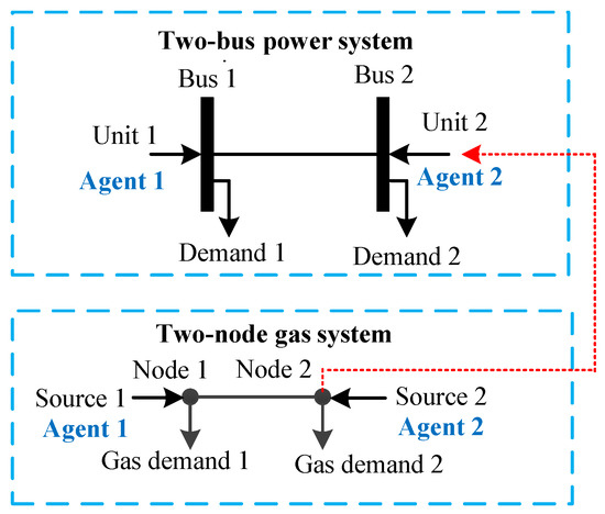
Figure 1.
Example: two-bus power system and two-node gas system.
We consider two hybrid agents:
- Agent 1 owns power unit 1 and gas source 1
- Agent 2 owns power unit 2 and gas source 2.
For simplicity, we do not consider strategic bids by consumers in this example. In addition, we consider a perfect gas price information interchange between the gas market and the owner of gas-fired power unit 2 (Agent 2).
5.1. Data
The capacities of the two power units at buses 1 and 2 are 50 MW and 20 MW, respectively. The marginal production cost of the power unit at bus 1 is 18 $/MWh. The non-fuel cost of the gas-fired unit at bus 2 is 1 $/MWh, and its energy conversion coefficient associated with gas consumption is 0.0045 .
Regarding the two gas sources at nodes 1 and 2, their capacities are 0.5 and 0.7 , respectively, and their marginal production cost are 3000 and 3500 , respectively.
The transmission capacity of the power transsmission line connecting buses 1 and 2 is 18 MW. The lower and upper gas pressure limits at gas nodes are 25 bar and 40 bar, respectively. We note that these gas nodal pressure bounds do not restrict the gas flows through the pipeline connecting nodes 1 and 2.
The baseline utility of the power demands at buses 1 and 2 are 30 $/MWh and 35 $/MWh, respectively. The baseline utility of the gas demands at buses 1 and 2 are 4000 and 4200 , respectively. The marginal utility factors of both gas and power demands during time periods 1–8, 9–16, and 17–24 are 0.8, 1.0, and 1.2 relative to their baseline utilities, respectively.
Finally, Figure 2 depicts the 24-h total non-generation-related gas demand and the total electricity demand.
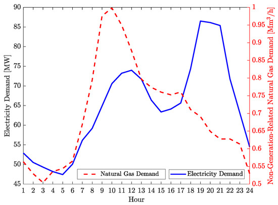
Figure 2.
Example: non-generation-related gas demand and power demand.
5.2. Results
We considered two equilibrium models (19)–(20), whose objective functions were total producers’ profit and social welfare of both markets, i.e., Max TPP EPEC, and Max SW EPEC, respectively. Table 1 summarizes the market equilibria obtained from the two models. We observed that the equilibrium model that maximized TPP yielded a lower SW but a higher TPP than the corresponding SW and TPP obtained from the equilibrium model that maximized SW. In addition, these two equilibrium models resulted in differences in the distribution of profits between the two production agents. Specifically, Agent 1 earned a higher profit from the model that maximized SW, while the model that maximized TPP was more beneficial for Agent 2.

Table 1.
Example: profits and social welfare ($ thousand) for two equilibrium models.
Additionally, we considered a gas-shortage case, where the capacity of gas-fired unit 2 was reduced to 10 MW. Table 2 provides results for the base case and the gas-shortage case obtained from the Max TPP EPEC. This table shows that the gas-shortage case resulted in a higher profit for Agent 1, earned from the electricity market. This is because power unit 1 accounted for an increased share of electricity supply. Additionally, the gas shortage resulted in lower profits for the two production agents earned from the gas market due to reduced generation-related gas demands.
Table 2.
Example: profits and social welfare ($ thousand) for two cases (Max Total Producers’ Profit (TPP) Equilibrium Problem with Equilibrium Constraints EPEC).
These results show how the operation of the gas system impacts production agents’ profits earned from both gas and power markets. In practice, gas-fired power producers should be aware of potential gas-system bottlenecks, which determine the availability and reliability of their fuel supply.
The EPEC model (19)–(20) was solved using BARON [24] under GAMS on a computer with a 2.1-GHZ Intel Core-i7 processor with 8 GB of memory. The solution time of any instance analyzed was below 190 seconds.
6. Case Study
This section examines a case study comprising the IEEE-57 bus system [25] and a tree-like 134-node Greek gas system (http://gaslib.zib.de/).
We consider (i) strategic offers/bids from both producers and consumers, (ii) disaggregated and aggregated gas price information, and (iii) diverse ownership of gas and power production units.
Taking into account the computational machinery used and for the sake of simplicity and tractability, we consider a time horizon of 3 h.
6.1. Data
The gas system consists of three gas sources, 45 demand nodes, 132 pipelines, and one gas compressor. The power system includes seven power units, being the units at buses 1, 2 and 3 gas-fired and connected to gas nodes 2, 8, and 15, respectively. This system includes 22 demand nodes and 80 transmission lines.
We consider three strategic agents, agents 1 and 2 being hybrid producers, and agent 3 a hybrid consumer. Specifically:
- Agent 1 owns the power units at buses 1–3 and 12, and gas sources at nodes 1 and 20.
- Agent 2 owns the power units at buses 6, 8, and 9, and the gas source at node 80.
- Agent 3 owns electricity demands at 10 buses and gas demands at 18 nodes.
All power units and gas sources are owned by either by Agent 1 or 2 and submit strategic offers. However, a number of electricity/gas demands are not owned by Agent 3, and hence bid competitively.
6.2. From Perfect to Oligopolistic Competition
Table 3 summarizes the market equilibria obtained from the competitive model and three oligopolistic models:
Table 3.
Case study: profits and social welfare ($ thousand) under different equilibrium models.
- Max SW EPEC.
- Max TPP EPEC.
- Max TCP EPEC.
Figure 3 and Figure 4 provide the load-weighted electricity and gas locational marginal prices (LMPs), respectively, obtained from the four models.
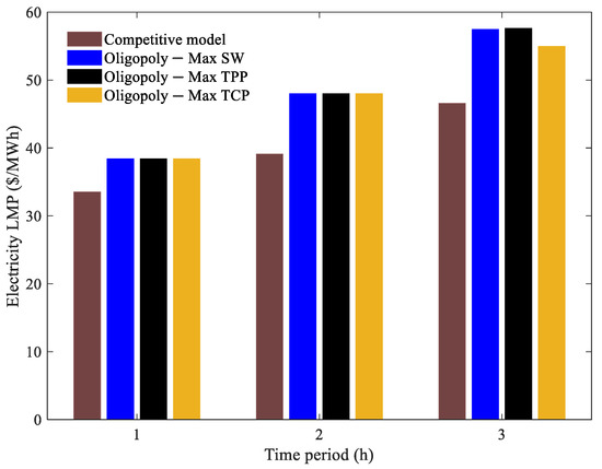
Figure 3.
Case study: load-weighted electricity locational marginal prices (LMPs) obtained from four equilibrium models.
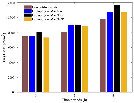
Figure 4.
Case study: load-weighted gas LMPs obtained from four equilibrium models.
The results obtained allow the following conclusions:
- Since no market power was exercised, the competitive model yielded the highest SW and the lowest electricity and natural gas LMPs.
- The oligopolistic model that maximized SW resulted in the same SW as the competitive one. However, the profits of the producers (Agents 1 and 2) obtained from the oligopolistic model were nearly twice those obtained from the competitive one.
- The oligopolistic model that maximized TPP resulted in lower SW but higher TP than the oligopolistic model that maximized SW. This is because the model that maximized TPP allowed producers further exercising market power, which yielded higher gas and power LMPs.
- The oligopolistic model that maximized TCP yielded the highest TCP, and the same SW than the oligopolistic model that maximized SW.
- Among the three oligopolistic models, the one that maximized TPP resulted in the highest gas and power LMPs, while the model that maximized TCP resulted in the lowest gas and power LMPs. Hence, supply-side market power increases energy prices, while the demand-side market power decreases them.
The EPEC models that maximized SW, TPP, and TCP required approximately 1681 s, 4123 s, and 3124 s, respectively, of wall-clock time to solve.
6.3. Aggregated Gas Prices
This subsection investigates the impact of temporal/spatial aggregation of gas prices on the market equilibria reached.
Considering the Max SW EPEC, Table 4 summarizes the market equilibria obtained from perfect pricing, spatial averaging pricing, temporal averaging pricing, and combined spatial and temporal averaging pricing.
Table 4.
Case study: profits and social welfare ($ thousand) for a perfect pricing and three imperfect pricing cases (Max SW EPEC).
The spatial averaging pricing derived a single price per hour by performing a load-weighting average across nodes of all gas LMP that hour (see (A32) in the Appendix). Similarly, the temporal averaging pricing derived a single price per node by performing a load-weighting average across hours of all gas LMP in that node (see (A33) in the Appendix). Finally, the combined spatial and temporal averaging pricing did both, deriving a single gas price per day (see (A34) in the Appendix).
We observe from Table 4 that the imperfect-pricing cases resulted in lower SW. Specifically, both spatial averaging pricing and temporal averaging pricing models yielded a lower TPP and a slightly higher TCP. However, the combined averaging pricing model resulted in a loss of both TPP and TCP.
These results show that highly granular pricing practices are desirable to co-ordinate gas and power markets. This is so because such practices prevent loss of SW and increased profits of gas/power producers.
6.4. Ownership Structure
We investigate in this section the impact of ownership structure on market equilibria. This was done by considering three cases involving all hybrid agents, some hybrid agents, and no hybrid agent. The Max TPP EPEC was considered. Table 5 describes the three cases considered.
Table 5.
Case study: ownership structure. A: power units at buses 1–3 and 12. B: power units at buses 6, 8, and 9. C: gas sources at nodes 1 and 20. D: gas source at node 80.
The resulting market equilibria are provided in Table 6. This table shows that the all hybrid agents’ cases resulted in the highest TPP and the lowest SW. In comparison, the case of no hybrid agent resulted in the lowest TPP and the highest SW. These changes in TPP and SW are due to differences in the market power exercised by gas/power producers. In the all hybrid agents’ cases, each agent accounted for a larger gas/power production capacity, and thus it could potentially exercise higher market power to its own profit, which, consequently, reduced the SW.
Table 6.
Case study: profits and social welfare ($ thousand) for different market ownership cases (Max TPP EPEC).
7. Case Study 2
This section summarizes numerical results from a realistic Belgian 24-node power system and 20-node gas system [17], the topology of which is shown in Figure 5. The power units at buses 2, 3, 6, 8, 16, 15, and 22 are gas-fired and connected to nodes 4, 3, 4, 4, 6, 11, and 13, respectively. We considered three strategic producers: agents 1, 2 and 3. Agent 1 owned power units in area 1 (see upper left-hand-side of Figure 5); agent 3 owned gas sources in area A (see upper right-hand-side of Figure 5); agent 2 owned power units in area 2 (see lower left-hand-side of Figure 5) and gas sources in area B (see lower right-hand-side of Figure 5). A fourth strategic agent owned electricity demands at buses 7, 9, 23, and 24 and gas demands at nodes 10, 12, 19, and 20. We considered a time horizon of 6 h.
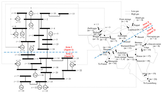
Figure 5.
Case study 2: Belgian 24-node power system and 20-node gas system.
We investigated the impact of gas-pressure limits on the market equilibria reached. This was done by comparing the results obtained from two cases, in which the ranges of nodal gas pressures were between 30 bar and 70 bar and between 35 bar and 65 bar, respectively. Table 7 and Figure 6 summarize the equilibrium results obtained from the two cases. These results indicate that a strict gas-pressure limit resulted in 1) a lower TPP, TCP, and SW, 2) higher gas LMPs, and 3) lower profits of agents 1 and 2 obtained from the power market owing to increased fuel cost for gas-fired units.
Table 7.
Case study 2: profits and social welfare ($ thousand) for two sets of gas pressure limits (Max TPP EPEC).
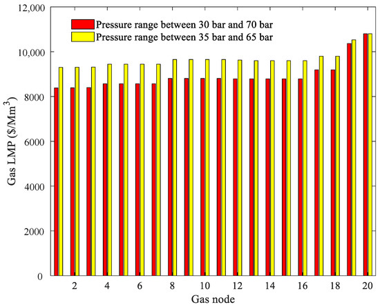
Figure 6.
Case study 2: gas LMPs at the peak time period for two sets of gas pressure limits (Max TPP EPEC).
8. Conclusions
This paper proposes a multi-period EPEC model to analyze the interactions of both strategic power/gas producers and power/gas consumers that participate in power and gas markets. We investigate the impacts of (i) market power, (ii) aggregated gas prices and (iii) ownership structure of power/gas producers on the market equilibria reached. From the analysis carried out, the conclusions below are in order:
- The proposed model is tractable and generally well-behaved, but complex. If larger instances and multi-period settings need to be considered, decomposition techniques and industry-grade computational resources are required.
- We verify with our model that the exercise of market power results in reduced social welfare and arbitrary allocation of the extra profits among market agents. Moreover, exercising market power in either the gas or the power market impacts both the power and gas markets.
- We find that bottlenecks in the gas system impact agents’ profits earned from both gas and power markets.
- Not transferring the true gas LMPs to the owners of gas-fired power units results in significant inefficiencies and potential intra-market and inter-market cross-subsidies.
- We verify that the ownership structure determines the degree of market power that can be exercised by market agents: the lower the intra- and inter-market concentration, the higher the efficiency.
- The model presented allows analyzing the impact of (i) a reduced disclosure of market outcomes (prices) and/or (ii) the impact of exercising market power by market agents. Such a model may help regulators to design market rules that encourages market-outcome disclosure, and discourages exercising market power.
Author Contributions
Conceptualization, A.J.C. and S.C.; methodology, A.J.C. and S.C.; software, S.C. and A.J.C.; validation, S.C. and A.J.C.; formal analysis, A.J.C. and S.C.; investigation, S.C. and A.J.C.; data curation: S.C. and A.J.C.; writing-original draft preparation, A.J.C. and S.C.; writing–review and editing, A.J.C. and S.C.; visualization, S.C. and A.J.C.; supervision, A.J.C. and S.C. All authors have read and agreed to the published version of the manuscript.
Funding
A. J. Conejo is partly supported by NSF Grant 1808169. S. Chen is partly supported by Fundamental Research Funds for the Central Universities under Grant 2019B05714.
Conflicts of Interest
The authors declare no conflict of interest.
Appendix A. Detailed Models
Appendix A.1. Gas Market Clearing
An SOC (Second Order Conic) formulation of the gas operation problem (3)–(5) is:
where e is the index of gas demands in set , t the index of operating periods in set T, l the set of agents in set , m and n the indices of nodes in set , v the index of power units, the set of gas-fired units connected to node m, the set of gas sources connected to node m, the set of gas compressors connected to node m, the set of gas demands connected to node m, the set of nodes that are connected directly to node m, k the index of gas compressors in the set , and w the index of gas sources.
The parameters of the problem (A1)–(A14) are described below. is the marginal utility of demand e at time period t, the gas transportation capacity of compressor k, the production capacity of gas source w, the quantity of gas demand e at time period t, the maximum gas consumption of power unit v, the line-pack parameter of the pipeline connecting nodes m and n, the Weymouth constant of the pipeline connecting nodes m and n, and the minimum and maximum compression ratio of compressor k, the conversion efficiency of gas compressor k, and and the minimum and maximum gas pressures of node m, respectively.
The variables of the problem (A1)–(A14) are as follows. is the consumption of demand e in time period t, the production of gas source w in time period t, the gas flow through compressor k in time period t, the gas flow through the pipeline connecting nodes m and n in time period t, the average gas flow through the pipeline connecting nodes m and n in time period t, the line-pack in pipeline connecting nodes m and n in time period t, the bid of demand e in time period t, the bid of gas-fired power unit v in time period t, and the offer of gas source w in time period t.
It should be noted that the variables , , and are fixed by upper-level problems and thus are constant for this problem. denotes the dual variable of (A2), and represents the gas LMP of node m at time period t. The variables of problem (A1)–(A14) are those in set .
The objective function (A1) is the gas SW that incorporates strategic offers from gas producers and strategic bids from power producers and gas consumers. Constraints (A2) represent the gas nodal balances. Constraints (A3) calculate average gas flows through pipelines. Constraints (A4) give the relationship between hourly changes in flows and line-pack in pipelines. Constraints (A5) determine the hourly line-pack in each pipeline, which is considered to be linear with the average gas pressure at the two ends of the pipeline. Constraints (A6) relate the average gas flow with the change in squared gas pressures between the upstream and downstream nodes for each pipeline. (A6) represent an SOC formulation of an exact gas flow model [3]. Constraints (A7) enforce minimum and maximum gas pressure ratios of gas compressors. Constraints (A8) impose transportation limits on gas compressors. Constraints (A9) and (A10) impose production capacities and ramping limits on gas sources, respectively. Constraints (A11) limit the amount of gas demands served. Constraints (A12) enforce minimum and maximum gas pressures of each node. Constraints (A13) assume that the direction of gas flows are known a priori, which is generally reasonable in short-term operations [3]. Constraints (A14) limit the amount of generation-related demands.
Appendix A.2. Power Market Clearing
An LP (Linear Programming) formulation of the power operation problem (6)–(8) is:
where d is the index of electricity demands in set , i and j the indices of electric buses in set , v the index of power units in set , the index of the reference bus. the set of strategic consumers owned by agent l, the set of non-strategic consumers, the set of electricity demands directly connected to bus i, the set of power units directly connected to bus i, and the set of buses directly connected to bus i.
The parameters of the problem (A15)–(A21) are described below. is the marginal utility of demand d in time period t, the susceptance of the line connecting buses i and j, the quantity of demand d in time period t, the transmission capacity of the line connecting buses i and j, and the capacity and ramping limit of power unit v, respectively.
The variables of the problem (A15)–(A21) are as follows. is the quantity of demand d served in time period t, the power production of unit v in time period t, the phase angle of bus i in time period t, the bid of demand d in time period t, and the offer of power unit v in time period t.
It should be noted that variables and are determined by upper-level problems and thus are constants for this problem. denotes the dual variable of (A16), and represents the electricity LMP of bus i in time period t. The variables of problem (A15)–(A21) are those in the set .
The objective function (A15) is the power SW that considers the strategic offers of power producers and the strategic bids of power consumers. Constraints (A16) represent the active power balances, in which the DC power flow model is used. Constraints (A17) impose upper limits on power demands. Constraints (A18) enforce the transmission capacity of each line. Constraints (A19) and (A20) impose production capacities and ramping limits on power units, respectively. Constraints (A21) fix the phase angle of the reference bus to zero.
Appendix A.3. Agent Model
Appendix A.3.1. Strategic Consumer
The problem of a gas/power strategic consumer is:
where is the bus at which electricity demand d is located, the node at which gas demand e is located, and .
The objective function (A22) is the profit of consumer l. Constraints (A23) and (A24) represent the non-negative bids of strategic gas consumer e and electricity consumer d, respectively. Constraints (A25) enforce market constraints.
Appendix A.3.2. Strategic Producer
The problem of a gas/power strategic producer is:
where is the bus at which power unit v is located, the gas price information that the gas system sends to power unit v, and the node at which gas source w is located, and .
The objective function (A26) is the profit of each producer l. Constraints (A27) and (A28) represent non-negative offers of power producer v and gas producer w, respectively. Constraints (A29) represent non-negative bids of gas-fired power unit v in the gas market. Constraints (A30) enforce market constraints.
Appendix A.4. Perfect and Imperfect Gas Price Disclosure
We consider perfect and imperfect price coordination between gas and power markets. Specifically, we consider different levels of gas price granularity. In the perfect-pricing case, exact gas price information is exchanged as:
where denotes the node at which gas-fired power unit v is located.
In the imperfect-pricing cases, we consider spatial, temporal, and combined averaging of gas LMPs, in which the information interchange on gas prices are given by (A32), (A33), and (A34), respectively.
Additionally note that the true SW is given by:
References
- Gil, J.; Caballero, A.; Conejo, A.J. Power Cycling: CCGTs: The Critical Link Between the Electricity and Natural Gas Markets. IEEE Power Energy Mag. 2014, 12, 40–48. [Google Scholar] [CrossRef]
- Chen, S.; Wei, Z.; Sun, G.; Cheung, K.W.; Sun, Y. Multi-linear probabilistic energy flow analysis of integrated electrical and natural-gas systems. IEEE Trans. Power Syst. 2017, 32, 1970–1979. [Google Scholar] [CrossRef]
- Chen, S.; Conejo, A.J.; Sioshansi, R.; Wei, Z. Unit Commitment with an Enhanced Natural Gas-Flow Model. IEEE Trans. Power Syst. 2019, 34, 3729–3738. [Google Scholar] [CrossRef]
- Byeon, G.; van Hentenryck, P. Unit Commitment with Gas Network Awareness. IEEE Trans. Power Syst. 2020. [Google Scholar] [CrossRef]
- He, C.; Zhang, X.; Liu, T.; Wu, L. Distributionally Robust Scheduling of Integrated Gas-Electricity Systems with Demand Response. IEEE Trans. Power Syst. 2019, 34, 3791–3803. [Google Scholar] [CrossRef]
- He, Y.; Yan, M.; Shahidehpour, M.; Li, Z.; Guo, C.; Wu, L.; Ding, Y. Decentralized Optimization of Multi-Area Electricity-Natural Gas Flows Based on Cone Reformulation. IEEE Trans. Power Syst. 2018, 33, 4531–4542. [Google Scholar] [CrossRef]
- Chen, R.; Wang, J.; Sun, H. Clearing and Pricing for Coordinated Gas and Electricity Day-Ahead Markets Considering Wind Power Uncertainty. IEEE Trans. Power Syst. 2018, 33, 2496–2508. [Google Scholar] [CrossRef]
- Ameli, H.; Qadrdan, M.; Strbac, G. Value of gas network infrastructure flexibility in supporting cost effective operation of power systems. Appl. Energy 2017, 202, 571–580. [Google Scholar] [CrossRef]
- Yang, J.; Zhang, N.; Kang, C.; Xia, Q. Effect of Natural Gas Flow Dynamics in Robust Generation Scheduling Under Wind Uncertainty. IEEE Trans. Power Syst. 2018, 33, 2087–2097. [Google Scholar] [CrossRef]
- Bai, L.; Li, F.; Jiang, T.; Jia, H. Robust Scheduling for Wind Integrated Energy Systems Considering Gas Pipeline and Power Transmission N–1 Contingencies. IEEE Trans. Power Syst. 2017, 32, 1582–1584. [Google Scholar] [CrossRef]
- Zlotnik, A.; Roald, L.; Backhaus, S.; Chertkov, M.; Andersson, G. Coordinated Scheduling for Interdependent Electric Power and Natural Gas Infrastructures. IEEE Trans. Power Syst. 2017, 32, 600–610. [Google Scholar] [CrossRef]
- Chen, S.; Wei, Z.; Sun, G.; Cheung, K.W.; Wang, D.; Zang, H. Adaptive Robust Day-Ahead Dispatch for Urban Energy Systems. IEEE Trans. Ind. Electron. 2019, 66, 1379–1390. [Google Scholar] [CrossRef]
- Antenucci, A.; Sansavini, G. Gas-constrained secure reserve allocation with large renewable penetration. IEEE Trans. Sustain. Energy 2018, 9, 685–694. [Google Scholar] [CrossRef]
- Ordoudis, C.; Pinson, P.; Morales, J.M. An Integrated Market for Electricity and Natural Gas Systems with Stochastic Power Producers. Eur. J. Oper. Res. 2019, 272, 642–654. [Google Scholar] [CrossRef]
- Wang, C.; Wei, W.; Wang, J.; Wu, L.; Liang, Y. Equilibrium of Interdependent Gas and Electricity Markets with Marginal Price Based Bilateral Energy Trading. IEEE Trans. Power Syst. 2018, 33, 4854–4867. [Google Scholar] [CrossRef]
- Wang, C.; Wei, W.; Wang, J.; Liu, F.; Mei, S. Strategic Offering and Equilibrium in Coupled Gas and Electricity Markets. IEEE Trans. Power Syst. 2018, 33, 290–306. [Google Scholar] [CrossRef]
- Chen, S.; Conejo, A.J.; Sioshansi, R.; Wei, Z. Equilibria in Electricity and Natural Gas Markets with Strategic Offers and Bids. IEEE Trans. Power Syst. 2020. [Google Scholar] [CrossRef]
- Ruiz, C.; Conejo, A.J. Pool Strategy of a Producer with Endogenous Formation of Locational Marginal Prices. IEEE Trans. Power Syst. 2009, 24, 1855–1866. [Google Scholar] [CrossRef]
- Ruiz, C.; Conejo, A.J.; Smeers, Y. Equilibria in an Oligopolistic Electricity Pool with Stepwise Offer Curves. IEEE Trans. Power Syst. 2012, 27, 752–761. [Google Scholar] [CrossRef]
- Chen, S.; Conejo, A.J.; Sioshansi, R.; Wei, Z. Operational Equilibria of Electric and Natural Gas Systems with Limited Information Interchange. IEEE Trans. Power Syst. 2020, 35, 662–671. [Google Scholar] [CrossRef]
- Ben-Tal, A.; Nemirovski, A. Lectures on Modern Convex Optimization: Analysis, Algorithms, and Engineering Applications; Society for Industrial and Applied Mathematics (SIAM): Philadelphia, PA, USA, 2001. [Google Scholar]
- Gabriel, S.A.; Conejo, A.J.; Fuller, J.D.; Hobbs, B.F.; Ruiz, C. Complementarity Modeling in Energy Markets; Springer: New York, NY, USA, 2013. [Google Scholar]
- Hu, X.; Ralph, D. Using EPECs to Model Bilevel Games in Restructured Electricity Markets with Locational Prices. Oper. Res. 2007, 55, 809–827. [Google Scholar] [CrossRef]
- Tawarmalani, M.; Sahinidis, N.V. A polyhedral branch-and-cut approach to global optimization. Math. Program. 2005, 103, 225–249. [Google Scholar] [CrossRef]
- Zimmerman, R.D.; Murillo-Sánchez, C.E.; Thomas, R.J. MATPOWER: Steady-State Operations, Planning, and Analysis Tools for Power Systems Research and Education. IEEE Trans. Power Syst. 2011, 26, 12–19. [Google Scholar] [CrossRef]
© 2020 by the authors. Licensee MDPI, Basel, Switzerland. This article is an open access article distributed under the terms and conditions of the Creative Commons Attribution (CC BY) license (http://creativecommons.org/licenses/by/4.0/).