Abstract
An accurate evaluation of the thermal transmittance (-value) of building envelope elements is fundamental for a reliable assessment of their thermal behaviour and energy efficiency. Simplified analytical methods to estimate the -value of building elements could be very useful to designers. However, the analytical methods applied to lightweight steel framed (LSF) elements have some specific features, being more challenging to use and to obtain a reliable accurate -value with. In this work, the main analytical methods available in the literature were identified, the calculation procedures were reviewed and their accuracy was evaluated and compared. With this goal, six analytical methods were used to estimate the -values of 80 different LSF wall models. The obtained analytical -values were compared with those provided by numerical simulations, which were used as reference -values. The numerical simulations were performed using a 2D steady-state finite element method (FEM)-based software, THERM. The reliability of these numerical models was ensured by comparison with benchmark values and by an experimental validation. All the evaluated analytical methods showed a quite good accuracy performance, the worst accuracy being found in cold frame walls. The best and worst precisions were found in the Modified Zone Method and in the Gorgolewski Method 2, respectively. Very surprisingly, the ISO 6946 Combined Method showed a better average precision than other two methods, which were specifically developed for LSF elements.
1. Introduction
The use of lightweight steel frame (LSF) systems has emerged as a viable alternative to traditional construction and its usage are increasing every year, mostly because of its great advantages, such as: cost efficiency, reduced weight, mechanical resistance, fast assemblage and others [1,2]. However, the high thermal conductivity of the steel could lead to thermal bridges effects resulting in a poor thermal performance of the building if those issues are not properly addressed (e.g., at design stage) [3].
A usual LSF wall is mainly composed of three parts: (1) steel frame internal structure (cold formed profiles); (2) sheathing panels (internal and external, e.g., gypsum plasterboard and OSB); (3) the insulation layers (cavity/batt insulation, such as mineral wool, and/or ETICS-exterior thermal insulation composite system) [3]. Notice that the batt insulation, besides the thermal insulation function, can also perform an important acoustic insulation function [4]. Moreover, the effectiveness of thermal insulation depends on its position in the LSF element [5], as well as on the type of LSF construction [6].
In fact, the existence of an insulation layer and its position on the wall determines the type of LSF construction. According to Santos et al. [1], a LSF construction element can be classified into three wall frame typologies: (1) cold, (2) hybrid, and (3) warm. On cold frame constructions, all the thermal insulation is placed inside the wall air cavity, between the vertical studs and limited to the stud depth. The opposite happens with the warm frame construction, where all thermal insulation is continuous and located outside of the steel frame (ETICS). Given its advantages, the hybrid construction type is used more often [4], being an intermediate solution between cold and warm construction and has both types of insulation applied: continuous exterior (ETICS) and between the steel studs (cavity insulation).
An accurate evaluation of the thermal transmittance (-value) of building envelope elements is fundamental for a reliable assessment of their thermal behaviour and energy efficiency [7]. LSF elements are even more challenging given the very reduced thickness of the cold formed steel profiles and the strong contrast between its thermal properties (e.g., thermal conductivity) and the thermal insulation materials (e.g., mineral wool) [8]. In buildings, despite thermal bridges originated by the high thermal conductivity of the steel frame [9], it is needed to account for flanking thermal losses around and in the intersection of building LSF components [10].
There are several approaches to obtain the thermal resistance/transmittance of building elements: (i) analytical, (ii) numerical, and (iii) measurements [11]. Regarding thermal performance measurements, they could be accomplished in-situ or in laboratory settings, being crucial for the validation of numerical and analytical methods [7]. In-situ non-destructive thermal transmittance measurements in existing buildings are very important for energy audit and retrofitting actions [7], which is very challenging to perform since the properties of materials are often unknown, components frequently degrade over time, and the experiments should be fast, simple and non-destructive [12]. Measurements under laboratory conditions have the advantages of well-known controlled environmental conditions, geometries, configurations and materials [7], but could be very time-consuming and expensive. There are various measurement methods, the most used ones being [7]: the heat flow meter (HFM) [13]; the guarded hot plate (GHP) [14]; the hot box (HB) [15], which could be calibrated (CHB) [16] or guarded (GHB) [17]; infrared thermography (IRT) [18].
Numerical simulations could be performed with more simpler two-dimensional (2D) models [5,6] or more complex/detailed three-dimensional (3D) models [9,10]. They have the advantage of allowing a quick comparison between several building component solutions/configurations. However, they need a specific software tool, skills to use it and to ensure the reliability of the obtained results the used models should be validated with measurements or at least verified by comparison with benchmark results.
The use of analytical formulas could be the simplest approach of all these three methods, being very useful and easy to use by designers [8]. However, this analytical approach is usually only available for simpler configurations; its applicability being, most often, very limited. Moreover, these analytical calculation formulations frequently consider a simplified steady-state one-dimensional (1D) heat transfer and do not take into account the heat storage inside the material, nor the thermal properties variation (e.g., with temperature or humidity) [19].
The use of analytical methods to calculate the thermal resistance (-value) and transmittance (-value) of a building element could be a complicated subject, especially when the element has inhomogeneous layers with very dissimilar thermal properties. For LSF constructions, those analytical calculations can be harder than in other forms of construction, as the methodology must include the effects of the non-homogeneous layers, the thermal bridges and the large difference between materials thermal conductivities [8].
One of the most used simplified analytical methods to calculate the thermal resistance and transmittance of a building component containing homogeneous and inhomogeneous layers is prescribed by standard ISO 6946 [20]. The total thermal resistance of a component is computed by combining its upper and lower limits, and thus this methodology is often designated as the ISO 6946 Combined Method. These -value limits are computed making use of the parallel path method (upper limit) and the isothermal planes method (lower limit). The total -value of the building element is calculated as the average of the upper and lower limits, as previously mentioned. However, this simplified analytical -value calculation methodology should not be applicable to building elements where the insulation is bridged by metal [20], as happens in cold and hybrid LSF elements.
This applicability limitation of the ISO 6946 Combined Method has motivated several researchers to seek for a specific analytical methodology suitable to calculate the - and -values for LSF building elements. The ASHRAE Zone Method [19] was one of the first analytical simplified methods to be developed to calculate the -value of a LSF element. The ASHRAE zone method is a modification of the parallel path method [21], where instead of considering only the thickness of the steel stud web, it considers a larger zone of influence of the metal thermal bridge within the LSF wall. The width of the area affected by the steel thermal bridge depends on the length of the steel stud flange and on the distance from this metal flange to the wall surface, i.e., the sheathing layers thickness [21].
Given the reported unsatisfactory accuracy of the ASHRAE Zone Method, Kosny et al. [21,22] developed a new improved methodology, often designated as Modified Zone Method [19]. This enhanced method to estimate the -value of metal frame walls was developed based on computer-simulation results and experimental measurements of different LSF wall configurations, taking into account several wall parameters, such as stud spacing, stud (depth) and flange sizes, stud metal thickness, the thermal resistance of the cavity insulation and thermal resistance of exterior sheathing [22]. It was concluded that the differences in the thermal calculations are caused by the metal stud zone area estimation. Thus, a more precise estimation technique to define the thermally affected zones caused by steel studs of LSF walls was developed and implemented.
More recently, Gorgolewski [8] adapted the ISO 6946 Combined Method to a more accurate analytical -value calculation methodology for LSF building components, including cold and hybrid frames. In this new suggested analytical methodology, the upper and lower -values limits are still being used, but instead of an average between these limits Gorgolewski found an “algorithm” for estimating the adequate weighting between them [8]. It was proposed and compared the accuracy of three analytical methods, being taken into account some parameters of the steel frame elements, such as flange width, stud spacing and stud depth. The third method developed by Gorgolewski was found to exhibit the best accuracy performance and thus it was adopted in the United Kingdom for LSF buildings code of practice [23].
As reviewed before, there are several analytical simplified methods available in the literature to compute the thermal resistance or transmittance of LSF building elements. However, it was not found in the bibliography any research work with the evaluation and comparison of the accuracy performance of these different analytical methodologies. Moreover, ISO 6946 [20] states that the prescribed Combined Method is not suitable to estimate the -value of cold and hybrid LSF elements, but it is not known how large is this methodology calculation error.
In this context, the main aim of this work—besides to perform a review of the analytical methods calculation procedures—is to evaluate and compare the accuracy of the above mentioned simplified analytical methods. With this goal, six analytical methods were used to estimate the thermal transmittance values of eighty different LSF walls. The obtained analytical -values were compared with those provided by numerical simulations, which were used as reference -values. The numerical simulations were performed using a 2D steady-state finite element method (FEM) based software, THERM [24]. The reliability of these numerical models was ensured via comparison with benchmark values. Additionally, an experimental validation of some LSF numerical models was also accomplished.
This paper is structured as follows. After this introduction, the six evaluated analytical methods are described, namely the ISO 6946 Combined Method, the three Gorgolewski methods and the two ASHRAE methods (zone and modified zone). Next, the numerical reference FEM models are described, including the benchmark verification and experimental validation, the boundary conditions used and the air-layer modelling. Subsequently, all the assessed 80 LSF walls are described, including the parameters evaluated, the variables changed and the values considered in the assessment; then we present the dimensions and thermal properties of the materials used in this study. Afterwards, the obtained results are presented and discussed. Finally, the main concluding remarks of this work are described.
2. Methods and Materials
2.1. Analytical Simplified Methods
As mentioned before, a building component could have homogeneous and/or inhomogeneous layers. When the building element is constituted by homogeneous plane layers (), which are perpendicular to the heat flow, the originated heat flow transfer is one-dimensional and the total thermal resistance (environment to environment) could be computed as prescribed by ISO 6946 [20],
where and are the internal and external surface resistances [], is the thermal resistance of each homogeneous layer . Notice that the results presented in Section 3 are thermal transmittances (-values), which were computed by the reciprocal of the total thermal resistance (), including the internal (0.13 ) and external (0.04 ) surface resistances, as prescribed by ISO 6946 [20] for horizontal heat flow.
When there are inhomogeneous layers in the building component, the heat flow starts being two-dimensional, instead of one-dimensional, given the different thermal conductivities and consequent different thermal resistances. These two-dimensional heat flow features get stronger when the discrepancies between the thermal properties of the materials (, conductivity) within the same layer are more significant.
There are several analytical simplified methods available to compute the thermal resistance or transmittance of building elements containing inhomogeneous layers (, LSF elements). In the next sections several analytical methods will be briefly described, namely: (1) ISO 6946 Combined Method [20]; (2) three methods proposed by Gorgolewski [8]; (3) ASHRAE Zone Method [19]; (4) ASHRAE Modified Zone Method [21].
2.1.1. ISO 6946 Combined Method
One of the most commonly used analytical simplified method to compute the thermal resistance of building elements consisting of homogeneous and inhomogeneous layers, which may contain air layers up to 0.30 m thick, is described in the international standard ISO 6946 [20] and therefore is often identified as ISO 6946 Combined Method, since the total thermal resistance () is computed by combining two different methods: (1) Parallel Path Method; (2) Isothermal Planes Method, as will be explained next.
According to ISO 6946 [20], this simplified analytical approach is only valid for the cases where the ratio of the upper limit to the lower limit of the thermal resistance does not exceeds 1.5. Furthermore, this method is not applicable to building elements where thermal insulation is bridged by metal (, steel studs), , when there is a significant difference between the thermal conductivity of the materials in the layer providing the most important thermal resistance of the building element. Thus, the ISO 6946 Combined Method (theoretically) is not valid for cold and hybrid LSF construction elements.
Moreover, ISO 6946 [20] prescribes (in Annex F) simplified corrections to the thermal transmittance values for: (1) air voids, (2) mechanical fasteners, and (3) inverted roofs, whenever the total correction exceeds 3%.
Upper Limit of the Total Thermal Resistance: Parallel Path Method
The upper limit of the total thermal resistance () is determined making use of the parallel path method, i.e., assuming one-dimensional heat transfer perpendicular to the surfaces of the building element.
This assumption is suitable when the materials on the same layer have close (, same order of magnitude) thermal conductivity values, as for example on wood frame walls [19]. As illustrated in Figure 1, usually two main paths are considered in stud cavity walls: Path , where the heat flux is typically higher given the higher thermal conductivity of the stud material and Path , with habitually lower heat flux given the lower thermal conductivity of the cavity insulation. Figure 1b displays these equivalent parallel path circuits for both paths.

Figure 1.
Parallel path method schematic illustration: (a) lightweight steel frame (LSF) wall cross-section; (b) Equivalent parallel path circuit.
This methodology does not take into account the steel stud horizontal parts (flanges) and stud returns, only considering the web of the stud, being the width of Section delimited by the web stud thickness.
Assuming these calculation principles, the upper limit of the total thermal resistance is given by Equation (2),
where and are the fractional areas of sections and , respectively, and are the total thermal resistances of each section/path []. These total thermal resistances are computed as the summation of the thermal resistances in series for each path (Figure 1b), , assuming homogeneous layers are perpendicular to the heat flow [20], including the internal and external surface thermal resistances.
Lower Limit of the Total Thermal Resistance: Isothermal Planes Method
The lower limit of the total thermal resistance () is determined by making use of the isothermal planes method, , by assuming that all planes parallel to the building element surface are isothermal surfaces. In this method, it is assumed that the heat can flow laterally in any component and the thermal resistances of adjacent components are combined in parallel, resulting on a path with series-parallel resistance combined [21]. This assumption is appropriate when adjacent materials of the same layer/plane have conductivity values moderately different, as with masonry walls [19]. Figure 2a illustrates the three layers (1, 2 and 3) and two sections ( and ) considered in a cold formed stud cavity wall. As mentioned before, given the batt insulation placed in the cavity, the thermal resistance of section (cavity insulation) is much greater than section (stud). As in the previously method (parallel path), only the web of the steel stud is considered for heat transfer calculation purposes.
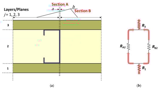
Figure 2.
Isothermal planes method schematic illustration: (a) LSF wall cross-section; (b) equivalent series-parallel circuit.
Figure 2b displays the equivalent series-parallel circuit assuming isothermal planes. Since layer 2 is inhomogeneous, both thermal resistances ( and ) are represented in parallel.
The calculation of the lower limit of the total thermal resistance is divided into two stages [20]. First, the equivalent thermal resistance () of each thermally inhomogeneous layer () is calculated (layer 2 for the wall in Figure 2) making use of the parallel path method according to Equation (3) [20], which could be simplified for the LSF wall illustrated in Figure 2, resulting in Equation (4).
Second, the lower limit of the total thermal resistance () is calculated as a summation of the series resistances,
including the equivalent thermal resistance of the inhomogeneous layer () previously obtained in Equation (4), as well as the internal and external surface thermal resistances.
Total Thermal Resistance: Combined Method
According with the ISO 6946 Combined Method, the total thermal resistance () is computed as an arithmetic average of the total upper () and lower () thermal resistances,
which means that the two -values (upper and lower limits) have the same weight (0.5) on the total resistance calculation [20].
2.1.2. Gorgolewski Methods
As the ISO 6946 Combined Method -value calculation excludes wall configurations—in which insulating layers are bridged by linear metal elements, like on lightweight steel frame (LSF) construction—from its scope, Gorgolewski [8] proposed three new methods based on similar principles used in that standard [20], adapting it to increase the accuracy for this type of construction. Using the same calculation methodology proposed on ISO 6946 to reach upper () and lower () limits of the thermal resistances, Gorgolewski’s method differs on the total resistance calculation by applying different weights for the upper and lower resistance values and considering a factor , between 0 and 1, such that the total thermal resistance () is given by Equation (7),
Thus, the total thermal resistances provided by the Gorgolewski methods ranges in the interval , as illustrated in the following expression,
being equal to the ISO 6946 total resistance when the -value is 0.5.
Notice that for warm LSF elements, , when there is only external insulation, it was assumed a p-value equal to 0.5 [23]. Thus, the obtained total thermal resistance for any of the Gorgolewski methods is equal to the one provided by ISO 6946 Combined Method [20].
The accuracy of the several methods proposed by Gorgolewski was verified by comparison to the results provided by 2D numerical FEM models for 52 different LSF walls and roof slabs [8].
Gorgolewski Method 1
The -value for the first (refined) method proposed by Gorgolewski [8] is expressed in Equation (9),
This -value depends directly on the ratio between the lower and upper limits of the total thermal resistance.
Gorgolewski Method 2
The -values for the second method proposed by Gorgolewski [8] are displayed in Table 1. These values take into account the stud spacing, having as reference 500 mm, and whether the LSF element is a hybrid or cold frame type.

Table 1.
Tabulated -Values for Gorgolewski Method 2 [8].
Analysing the proposed p-values, being all of them lower or equal to 0.5, and looking to Equation (7), it can be concluded that the total thermal resistance predicted by this method will be closer to the lower limit, , for cold frame construction or whenever the stud spacing is lower than 500 mm. This is to be expected, given the higher amount of thermal insulation bridged by steel webs and the higher amount of steel, respectively, thus reducing the overall thermal resistance of the LSF element.
Gorgolewski Method 3
The -value for the third method developed by Gorgolewski [8] is derived from the previous ones and it is expressed in Equation (10),
As with Method 1 (Equation (9)), the -value directly depends on the ratio between the lower and upper limits of the total thermal resistance. Additionally, besides the constant 0.44 parcel, there are more three variables, namely: the flange length (), the stud spacing () and stud depth (), all dimensions of which are given in metres [m].
2.1.3. ASHRAE Methods
Some of the previously described methods (e.g., parallel path method) assume that the heat flow is perpendicular to the wall. Although when the wall structure contains steel framing members next to materials with low thermal conductivity (, thermal insulation), the two-dimensional effects caused by thermal bridges become more relevant [21]. The ASHRAE methods were developed for structures with widely spaced metal members of substantial cross-sectional areas and when the adjacent materials have very high different conductivities (two order or more of magnitude), as what happens on typical LSF constructions [19].
The ASHRAE methods are an adjustment of the parallel path method, where an area “weighting factor” is applied to the wall section influenced by the steel stud thermal bridge [21]. This section is defined by the width of the steel thermal bridge influence zone (Figure 3) and, thus, it is named section . The remaining portion of the wall cavity without the thermal bridge influence it is called section .
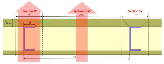
Figure 3.
LSF wall cross-section illustration for the ASHRAE methods: Sections W and CAV.
The section W represents the area where the metal stud has influence on the heat path, being centred on the metal part of the wall cross-section and its length, , is determined by,
where is the flange length [m], is the zone factor (which will distinguish both ASHRAE methods as explained in the following sections) and is the thickness [m] of the thicker sheathing side (internal or external).
For both sections paths, the thermal resistances values are computed and them combined using the parallel path method and the average thermal transmittance per unit overall area is calculated by reversing the total thermal resistance [19], as detailed in the next subsection.
ASHRAE Zone Method
The first method proposed by ASHRAE, the Zone Method, uses Equation (11) to calculate the length of section and the zone factor, , is equal to 2.0. The remaining calculations for total thermal resistance and transmittance are the same for both ASHRAE methods and will be presented next. The detailed dimensions of Section W, which were already presented in Figure 3, are illustrated in Figure 4a. Moreover, the equivalent series-parallel circuit used in the simplified heat transfer calculations is displayed in Figure 4b. Notice that the steel frame is taken into account in the web and both flanges, though is neglected at the steel lip/return.
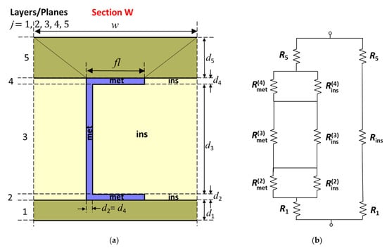
Figure 4.
ASHRAE methods schematic illustration: (a) Section W of the LSF wall cross-section; (b) Equivalent series-parallel circuit.
The total thermal resistance, , of a generic LSF wall displayed in Figure 3 is computed by applying the parallel path method to both considered sections (W and CAV),
where and are the total thermal resistances [] of sections W and CAV, respectively, and are the lengths [m] of sections W and CAV, respectively, and is the studs spacing [m].
The total thermal resistance of the homogeneous layers of the LSF wall cavity, , is calculated as the summation of the thermal resistances of all the layers in series, including the internal and external surface thermal resistances,
where is the thermal resistance of the insulation layer [].
The total thermal resistance of the Section W, , is computed making use of the isothermal planes method. First, the equivalent thermal resistance () of each thermally inhomogeneous layer () is calculated making use of the parallel path method to both metal () and insulation () materials,
Next, these three equivalent thermal resistances are used to compute the total thermal resistance of Section W, having taken into account all the five layers considered, including the ones for the sheathing homogeneous layers ( and ), as well as the surface thermal resistances,
Modified Zone Method
The Modified Zone Method is very similar to the Zone Method, making use of the same equations (Equations (12)–(17)). However, it uses a modified zone factor () value, which is not a constant, nor necessarily equal to 2. In the Modified Zone Method, the width () of the steel stud influence zone (Section W in Figure 3), besides the flange length, , depends on three parameters [19]: (1) the ratio between thermal resistivities of sheathing material and cavity insulation material; (2) the size (depth) of the stud; (3) thickness of the sheathing material.
The modified zone factor, , is usually obtained from a chart [19] (when the thickness of the sheathing materials is higher than 16 mm) and depends on the ratio between the average resistivity of the external sheathing material () and cavity insulation material () for the first 25 mm, combined with the stud size (usually one curve for each stud type). Notice that the thermal resistivity of a material is the reciprocal of its thermal conductivity , i.e., .
In this work, the authors adjusted two power trend-lines to the points obtained from reference [19] for C90 and C150 steel studs, as illustrated in Figure 5. The R-squared determination coefficient was very good, , equal to 0.999 in both curves. These power functions were used in the computations for both steel profile sizes (C90 and C150). The authors were not able to find the modified zone factor curves/points for C170 and C200 studs. Thus, it was assumed by approximation that the C170 factors were similar to the ones provided by the C150 curve. Regarding the LSF walls with C200 steel studs, they were not computed by this method in this work (only five LSF walls).

Figure 5.
Modified zone factor curves for LSF walls with cavity insulation whenever the total thickness of sheathing materials is higher than 16 mm.
The condition for using the chart presented on Figure 5 is that—for at least one of the sides of the wall—the total thickness of the sheathing layers must be thicker than 16 mm. If both interior and exterior sheathings have a total thickness smaller than 16 mm, the values should be obtained according to the following conditions [19]:
2.2. Numerical Reference 2D FEM Computations
There are several numerical computational methods that are able to reproduce highly detailed models of building components and accurately calculate and predicted their thermal behaviour under pre-established conditions. The numerical computational tool used in this work was the 2D FEM software, THERM [24]. For all LSF wall models the maximum error admitted on the FEM computations was 2%.
2.2.1. Accuracy Verification and Models Validation
The accuracy of THERM models used for the LSF wall thermal performance evaluation was checked under two different verifications: (1) benchmark values for two test cases presented on ISO 10,211 [25], and (2) comparison with the analytic -value provided for a wall assuming homogeneous layers. Despite the fulfilled verifications, a validation with laboratorial measurements was also performed.
ISO 10,211 Test Cases Verification
To verify the accuracy of 2D calculation algorithms, the standard ISO 10,211 [25] provides, in Annex C, two test reference cases (Case 1 and 2). According with these 2D standard test cases, the FEM THERM software [24] is classified as a steady-state high precision algorithm. The authors also implemented two test cases to ensure and demonstrate their ability to accurately make use of this software to model heat transfer problems. In both test cases, the difference between the standard solution given for each point and the temperature computed by the algorithm should not exceed 0.1 °C [24]. In test case 1, we provided a sketch of a half square column with 28 grid points placed equidistantly, for which the corresponding temperatures for each point are known (Figure 6a). Figure 6b displays the temperature values calculated by THERM in these reference grid points, all of them being equal to the ones provided by ISO 10,211 when using one decimal place temperature values.
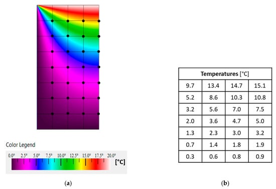
Figure 6.
ISO 10,211 obtained results for test case 1: (a) Temperature distribution and reference grid points; (b) Computed temperatures at reference grid points.
In the second test case, the difference between the heat flow calculated and the reference value shall not exceed 0.1 W/m. Figure 7a illustrates the computed temperature distribution, as well as the points where the reference temperatures are provided (points A to I). Figure 7b displays the previously mentioned computed temperatures and the heat flow calculated by THERM for this model. For all reference points, the temperatures obtained were exactly the same as prescribed by ISO 10211. The calculated heat flow rate was only 0.01 W/m lower the reference value (9.5 W/m), but still far below the difference limit of 0.1 W/m.
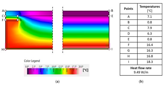
Figure 7.
ISO 10,211 test case 2 obtained results: (a) Temperature distribution and reference points; (b) Computed values.
Homogeneous Wall Layers Verification
An additional simple verification that was made was to compare the analytical and the numerical results for a simplified model of the LSF wall, i.e., the same wall composed only for homogeneous layers (without the steel studs). For those homogeneous walls, the analytical solution is known, being the total thermal resistance calculated as a sum of the layer’s resistances as described in Equation (1).
For this verification, the LSF wall (defined in Section 2.3) was used as a reference, but without steel studs. The numerical simulation result provided by THERM was = 0.227 W/(m2·K). As expected, a simple analytical approach for the same homogeneous wall brings up exactly the same thermal transmittance result.
Experimental Lab Measurements Validation
To validate the numerical simulation results provided by THERM software, used as reference values to evaluate the accuracy of the analytical methods, the thermal transmittance (-value) of some LSF walls were measured on a laboratory facility. In these experiments it was used the heat flow meter method, prescribed in standard ISO 9869-1 [13]. To ensure a controlled temperature gradient between the two surfaces of the LSF wall test-specimen two small thermally insulated boxes were used (Figure 8): (1) a hot box, heated by an electrical resistance (70 watts), and (2) a cold box, cooled by a refrigerator attached to it (Figure 8b). The steady-state set-point temperatures considered in the hot and cold boxes were 40 °C and 5 °C, respectively.
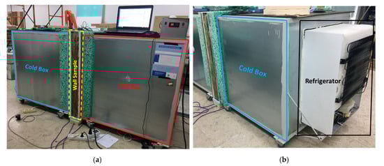
Figure 8.
Mini hot box apparatus: (a) Cold and hot boxes with the wall sample; (b) Refrigerator attached to the cold box.
The wall test samples used in these measurements have the following height and width dimensions: 1030 × 1060 mm, respectively, and the stud spacing was equal to 400 mm, as illustrated in Figure 9a. The cold formed steel profiles used in these experiments have a type C cross-sectional shape and have the following dimensions: C90 × 43 × 15 × 1.5 mm.
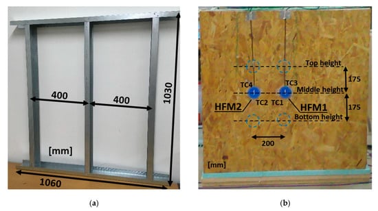
Figure 9.
LSF small-scale test sample wall: (a) Steel frame; (b) Sensors locations on exterior wall surface (HFM–Heat flux meter; TC-Thermocouples).
Four heat flux meters (Hukseflux HFP01, precision: ±3%) were used in these LSF wall experiments, being the measurements performed at four different locations: two at the hot surface and the remaining two at the cold wall surface. In both test-specimen wall surfaces a measurement location was chosen in the vicinity of the vertical steel stud (HFM1) and another one in the middle of the insulation cavity (HFM2), as illustrated in Figure 9b.
The temperatures were measured making use of 12 thermocouples (TC), certified with class 1 precision, with half of them being used in each side of the wall (hot and cold). From these six TC, two measured the environment air temperature inside each box (TC5 and TC6), another two measured the air temperature between the radiation shield and the wall surface (TC3 and TC4), while the remaining two measured the wall surface temperatures (TC1 and TC2), as illustrated in Figure 9b.
In order to ensure the repeatability of the experimental measurements, one test was performed for each wall at three height locations (Figure 9b): (1) top, (2) middle, and (3) bottom, the average of these three tests being the considered measured -value of the LSF wall. Each test had a duration of 24 h.
The data recorded during the experiments (temperatures and heat fluxes) were recorded in two PICO TC-08 data-loggers (precision: ±0.5 °C); one for each side of the LSF wall test-specimen (hot and cold). Making use of the data recorded (heat fluxes and temperatures) and applying the HFM method, prescribed in standard ISO 9869-1 [13], two distinct -values were obtained: (1) a higher value for location 1, i.e., in the vicinity of the steel studs, and (2) a lower value between the steel studs, i.e., in the middle of the insulation cavity. The overall -value of the wall was obtained by computing an area weighted of both -values. The steel stud influence zone area was defined as prescribed by ASHRAE zone method.
Two LSF walls were tested to validate the numerical simulations: (1) an air cavity wall, and (2) a Mineral Wool (MW) insulation filled cavity wall. All the other exterior and interior sheathing materials were the same, i.e., an outer and an inner OSB layer (12 mm), attached to the C90 steel studs, as well as a Gypsum Plaster Board (GPB), this being the innermost layer (12.5 mm).
Table 2 display the obtained overall -values measured under controlled laboratory conditions (three tests for each wall) and the predicted values by 2D FEM numerical simulations.
Table 2.
Thermal Transmittance Values Measured in Lab and Computed by 2D FEM Numerical Simulations (THERM).
The -value predicted by the numerical simulations for the MW LSF wall exactly matches the measured one (0.621 W/(m2·K)), while for the air cavity LSF wall it was found to have an error of about 2%—the predicted -value (1.931 W/(m2·K)) being slightly lower than the measured one (1.969 W/(m2·K)). Given the uncertainties related to the measurements (e.g., sensor precision and material properties) and the maximum error estimated for the FEM numerical simulations (under 2%), these results allowed to reiterate and ensure the reliability of the numerical simulations used in this work as reference values.
2.2.2. Boundary Conditions
In this section are briefly presented the boundary conditions used in the numerical simulations of the LSF wall cross-sections. The temperatures for the inside warm and outside cold environments were set to 20 °C and 0 °C, respectively. The surface thermal resistance values used in the simulations were obtained from ISO 6946 [20] for horizontal heat flow (walls): 0.13 (m2·K)/W for internal thermal resistance () and 0.04 (m2·K)/W for external thermal resistance (). Additionally, two adiabatic surfaces were defined in both extremities of the LSF wall model cross-section.
2.2.3. Air Layers Modelling
Some LSF walls evaluated do not present a full-filled insulation cavity or have an empty air cavity, being necessary to model air gaps inside the LSF wall. The thermal resistances of those unventilated air layers were modelled with a solid-equivalent thermal conductivity, using the thermal resistance values prescribed by ISO 6946 [20] for horizontal heat flow.
2.3. Walls Description and Material Characterization
In this work, all the evaluated walls were derived from a typical reference exterior LSF wall (hybrid frame construction), as illustrated in Figure 10 and described in Table 3. The vertical steel studs (C90 × 43 × 15 × 1.5 mm) were spaced 600 mm apart. The exterior sheathing was constituted of an oriented strand board (OSB) panel (12 mm thick), while the external thermal insulation composite system (ETICS) was made of EPS (Expanded Polystyrene), 50 mm thick. The interior sheathing was made of an OSB panel (12 mm) and a gypsum plaster board (GPB), 12.5 mm thick, while the air cavity was filled with mineral wool (MW) batt insulation.
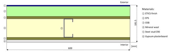
Figure 10.
Reference LSF wall cross-section materials and dimensions.
Table 3.
Reference LSF Wall Material Thickness () and Thermal Conductivities ().
Modifying some parameters and variables (listed on Table 4) on the reference LSF wall (Figure 10), eighty different LSF walls models were obtained. The evaluated parameters were the cold formed steel studs, the cavity insulation, the exterior continuous insulation and the studs facing sheathing materials.
Table 4.
Evaluated Parameters, Variables and Values Used in the Simulations, and Range of Obtained Thermal Transmittances (-Values).
Regarding the steel studs, four different values were modelled for the spacing (300–800 mm range) and depth (90–200 mm range) of the studs. Five different values for the steel studs thickness were evaluated, ranging from 0.6 mm up to 2.0 mm. Two different studs flange lengths were modelled: 43 and 70 mm, as obtained from the Pertecno cold-formed steel profiles manufacturer catalogue [32].
Concerning the cavity insulation thickness, three different levels of batt insulation were evaluated for each one of the four assessed steel studs (C90, C150, C170 and C200): (1) no cavity insulation; (2) half of the cavity filled with batt insulation; (3) cavity full filled with batt insulation. Moreover, two different batt insulation materials were considered: (1) the reference one, , mineral wool (MW) with thermal conductivity equal to 0.035 W/(m·K), and (2) a better performance insulation material (aerogel insulation blanket-AIB) with 0.018 W/(m·K).
Regarding exterior continuous insulation, eight different thicknesses were evaluated, ranging from 0 mm up to 80 mm. Furthermore, two different materials were considered: (1) the reference one, , EPS with thermal conductivity equal to 0.036 W/(m·K), and (2) a worst performance insulation material (insulation cork board-ICB) with 0.045 W/(m·K).
Finally, concerning the sheathing parameter, besides the OSB and GPB panels, three different materials were evaluated, namely cement wood board (CWB), fibre cement board FCB and glass-fibre reinforced board (GRB). The thermal conductivities of these sheathing materials ranges from 0.100 W/(m·K) for OSB up to 0.500 W/(m·K) for GRB.
Usually LSF walls are grouped into warm, hybrid and cold frame construction depending on the thermal insulation type/location, i.e., cavity batt insulation and/or exterior continuous thermal insulation [1]. Table 5 displays the total number of LSF walls evaluated (80) as well as the number of LSF walls by frame type: Warm (22 walls), Hybrid (43 walls), and Cold (15 walls). Additionally, this table also shows the range of -values evaluated, being the minimum thermal transmittance equal to 0.153 W/(m2·K) for a hybrid frame construction, while the maximum value is 0.983 W/(m2·K) for warm frame construction.
Table 5.
Number of Evaluated LSF Walls by Frame Type and Range of Obtained Thermal Transmittances (-values).
3. Results and Discussion
3.1. All LSF Walls
The -values obtained by the six analytical methods for all the evaluated LSF walls are plotted on Figure 11. Each point in these graphics represents a different LSF wall, being the value on the horizontal axis the reference -value provided by the numerical 2D FEM simulations, while the value on the vertical axis is the analytical -value estimated by the respective method: (a) ISO 6946 Combined Method; (b) Gorgolewski Method 1; (c) Gorgolewski Method 2; (d) Gorgolewski Method 3; (e) ASHRAE Zone Method; (f) Modified Zone Method.
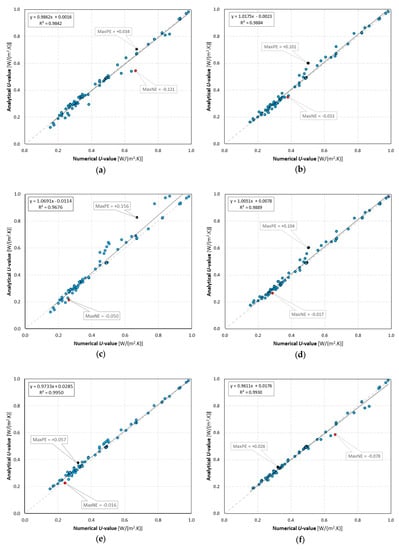
Figure 11.
Thermal transmittances (-values) comparison between the evaluated analytical methods and the numerical 2D FEM results used as reference: (a) ISO 6946 Combined Method; (b) Gorgolewski Method 1; (c) Gorgolewski Method 2; (d) Gorgolewski Method 3; (e) ASHRAE Zone Method; (f) Modified Zone Method.
Moreover, these plots also display a linear trend-line, the R-squared coefficient of determination, the maximum positive error (MaxPE), as well as the maximum negative error (MaxNE) for each analytical method, as well as a 45 degrees’ inclination line, that corresponds to the plots position for a virtual perfect match between the analytical and the numerical methods.
First of all, it could be concluded that there is a quite good agreement between the -values provided by the analytical methods evaluated and the numerical reference ones, evidencing a pretty good accuracy of these analytical methods.
Gorgolewski Method 2 (Figure 11c) exhibits a larger dispersion of values mainly for higher -values (greater than 0.4 W/(m2·K)). This feature is ensured by the linear trend line, which has the biggest slope (1.0691), being above the 45° diagonal line and—even so—exhibiting the smallest determination coefficient (0.9676). Additionally, a major positive error was also found in this analytical method (+0.156 W/(m2·K)). This LSF wall is cold framed (without ETICS), having the air cavity 50% filled with mineral wool.
Moreover, the major negative error (−0.121 W/(m2·K)) was found in the ISO 6946 Combined Method (Figure 11a). This LSF wall is cold-framed (without ETICS), having GRB sheathing panels. Quite surprisingly, this analytical method provides pretty good accuracy, since according with standard ISO 6946 [20] it should not be applicable to building elements where the insulation is bridged by metal, as happens in these cold and hybrid LSF walls.
Looking to both ASHRAE methods (Figure 11e,f), though they have different trends, they both have a very good determination factor (0.995 and 0.993). The ASHRAE Zone Method (Figure 11e) has a very good precision for higher -values (e.g., >0.6 W/(m2·K)), whereas for lower values exhibits a conservative trend, i.e., giving -values bigger than the real ones. On the other hand, the Modified Zone Method (Figure 11f) has a good precision for lower -values (e.g., <0.6 W/(m2·K)), but for lower values exhibits an overoptimistic trend, i.e., -values smaller than the real ones.
Notice that the linear trend-lines presented before and the corresponding determination factors are not the most adequate features to accurately quantify the precision of each analytical method, since they do not correlate the analytical -values with the numerical reference ones, but instead they correlate the analytical values with the corresponding trend-line, which could be very different from the 45° diagonal line.
Thus, it was decided to also compute the root mean square error (RMSE), as an absolute value and as a percentage, which is graphically displayed in Figure 12. These plots also contain the maximum positive errors (MaxPE) and the maximum negative errors (MaxNE).
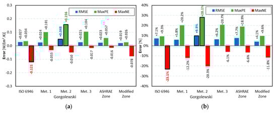
Figure 12.
-values errors for all LSF walls: (a) Absolute errors; (b) Percentage errors.
The Gorgolewski Method 2 exhibits the major RMS error (+0.048 W/(m2·K); +9.9%), as well as the higher maximum positive error (+0.156 W/(m2·K); +28.1%), confirming the relatively bad accuracy performance of this method. As mentioned before, the maximum negative error was found in the ISO 6946 Combined Method (−0.121 W/(m2·K); −23.1%).
Looking now to the smaller RMS error, the lowest value was found for the Modified Zone Method (+0.019 W/(m2·K); +4.1%). This analytical method also exhibits the lowest absolute MaxPE (+0.026 W/(m2·K)) and the second lowest percentage MaxPE (+9.6%), confirming the relatively good accuracy performance of this method. The lowest absolute negative error was found in the ASHRAE Zone Method (−0.016 W/(m2·K)), while the lowest percentage value was found in the Gorgolewski Method 3 (−6.1%).
Taking into account only the RMSE percentage values, the accuracy performance of these analytical methods could be ranked, from the better to the worst, as follows: (1) Modified Zone Method (+4.1%); (2) Gorgolewski Method 1 (+5.8%); (3) Gorgolewski Method 3 (+6.2%); (4) ISO 6946 Combined Method (+7.1%); (5) ASHRAE Zone Method (+7.7%); (6) Gorgolewski Method 2 (+9.9%).
In the following sections, a similar analysis will be performed, but separating the LSF walls into groups, depending on the frame type: (1) warm; (2) hybrid; (3) cold.
3.2. Warm Frame Walls
Figure 13 shows the absolute and percentage thermal transmittance error values obtained for the warm frame walls. Comparing these values with the previous ones (Figure 12), the first remarkable feature is that these error values now appear too small. This is justifiable by the existence of only continuous external thermal insulation (ETICS), existing no insulation in the air cavity between the steel studs and therefore without any thermal bridge effect.
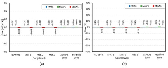
Figure 13.
-values errors for warm frame walls: (a) Absolute errors; (b) Percentage errors.
The errors are so small in absolute values, ranging between +0.006 W/(m2·K) and −0.004 W/(m2·K), as well as in percentage (+1.2%; −0.5%), that it does not worth it to make a more detailed analysis.
3.3. Hybrid Frame Walls
Figure 14 illustrates the error values obtained for the hybrid frame walls. These error values are considerably higher when compared to the previous warm frame ones (Figure 13). This is to be expected, as besides the continuous external thermal insulation, there is also batt insulation which is bridged by the steel studs.
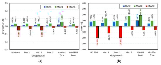
Figure 14.
-values errors for hybrid frame walls: (a) Absolute errors; (b) Percentage errors.
In these hybrid frame walls, the major -value RMS error was obtained by the ASHRAE Zone Method (+0.021 W/(m2·K); +9.7%), as well as the higher maximum positive error (+0.057 W/(m2·K); +18.9%), showing a relatively bad accuracy performance of this method. The maximum negative error was achieved by both ISO 6946 Combined Method and Gorgolewski Method 2 (−0.050 W/(m2·K); −20.3%).
The minor -value RMS error was obtained by the Modified Zone Method (+0.012 W/(m2·K); +4.6%), exhibiting also the lowest absolute positive error (+0.026 W/(m2·K)) and the smaller percentage negative error (−6.0%), demonstrating the relatively good accuracy of this analytical method for hybrid frame walls.
Having taken into account only the RMSE percentage values, the accuracy performance of these analytical methods, regarding the computation of hybrid frame walls -values, could be ranked, from the better to the worst, as enumerated next: (1) Modified Zone Method (+4.6%); (2) Gorgolewski Method 1 (+5.6%); (3) Gorgolewski Method 3 (+6.1%); (4) ISO 6946 Combined Method and Gorgolewski Method 2 (+7.9%); (5) ASHRAE Zone Method (+9.7%).
3.4. Cold Frame Walls
The thermal transmittance error values for cold frame walls are displayed in Figure 15. In general, these error values are even higher than the ones obtained for hybrid fame walls (Figure 14). These could be explained by the fact that all thermal insulation of the LSF wall is now bridged by the steel studs, exhibiting no continuous external thermal insulation (ETICS).
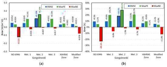
Figure 15.
-values errors for cold frame walls: (a) Absolute errors; (b) Percentage errors.
The major -value RMS error was obtained by the Gorgolewski Method 2 (+0.106 W/(m2·K); +18.4%), as well as the higher maximum positive error (+0.156 W/(m2·K); +28.1%), showing a relatively bad accuracy performance of this method. However, the maximum negative error is the smaller one (−0.007 W/(m2·K); −1.9%). These two facts suggest that this analytical method tends to provide much too conservative -values—i.e., higher than the real ones—originating from a relatively lower precision performance.
The maximum negative error was found in the ISO 6946 Combined Method (−0.121 W/(m2·K); −23.1%), evidencing that this method could provide significant overoptimistic -values, i.e., lower than the real ones, being this trend already seen also for hybrid frame walls (Figure 14).
Observing now the lowest -value RMS errors, the smaller error was obtained by the ASHRAE Zone Method in absolute value (+0.032 W/(m2·K) and by the Modified Zone Method in percentage value (+5.4%). The Modified Zone Method also exhibits the lowest maximum positive error (+0.015 W/(m2·K); +3.9%), revealing also in this parameter a relatively good accuracy performance. Another interesting feature is that all the errors provided by the ASHRAE Zone Method are positive, the minimum value being equal to +0.001 W/(m2·K) and +0.1%, showing a conservative trend.
Taking into account only the RMSE percentage values obtained for the cold frame walls, the accuracy performance of the evaluated analytical methods could be ranked, from best to the worst, as listed next: (1) Modified Zone Method (+5.4%); (2) ASHRAE Zone Method (+6.5%); (3) ISO 6946 Combined Method (+9.3%); (4) Gorgolewski Method 1 (+9.6%); (5) Gorgolewski Method 3 (+10.0%); (6) Gorgolewski Method 2 (+18.4%).
3.5. Overview
In order to provide a better perception and an easier comparison between the average accuracy performance of the six analytical methods evaluated, Figure 16 displays the percentage RMS errors for all LSF walls and also grouped by frame types.
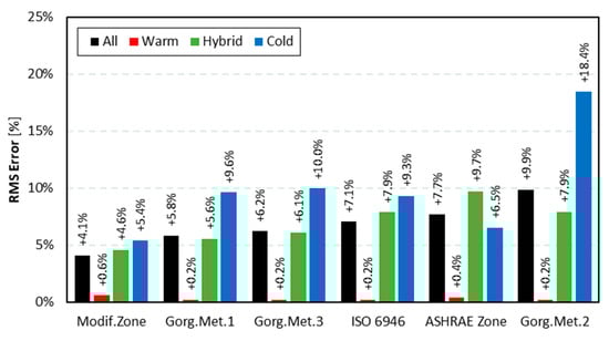
Figure 16.
Root mean square -values errors obtained for the evaluated analytical methods.
Looking to the four grouped RMSE values and comparing their relative values, the highest RMS percentage errors occur in the cold frame walls, followed by the hybrid frame walls (which exhibits values relatively closer to all LSF walls) and by the warm frame walls. There is only one exception: the ASHRAE Zone Method, where the higher error is in the hybrid frame (9.7%) instead of in the cold frame (6.5%). As mentioned before, this trend is related to the amount of thermal insulation that is bridged by the steel frames, which increases the error of the analytical methods in cold frame walls, the error being significantly reduced when there is only continuous external insulation (warm frame walls).
The major RMS -value error occurred in cold frame walls evaluated by the Gorgolewski Method 2 (18.4%), while for the same frame type the smaller error occurs in the Modified Zone Method (5.4%).
Regarding the most common LSF wall type (hybrid frame), the major error occurred in the ASHRAE Zone Method (9.7%), while the smaller error happened in the Modified Zone Method (4.6%), confirming the relatively good accuracy performance of this method.
Observing all the LSF walls evaluated, the RMS -value errors ranges between 4.1% (Modified Zone Method) and 9.9% (Gorgolewski Method 2). According to these RMS -value errors, the accuracy performance of the evaluated methods could be ranked as displayed in Figure 16 horizontal axis from the left (better) to the right (worst), being this ranking previously presented in Section 3.1.
In order to assess the statistical significance of the previously presented percentage -values errors, Table 6 displays the standard deviations and the confidence intervals (upper and lower limits, and amplitude) for each evaluated analytical method, computed for a level of significance equal to 5%, i.e., for a 95% confidence level. The standard deviation ranges from 4.0% (Modified Zone Method) up to 9.4% (Gorgolewski Method 2), while the amplitude of the confidence intervals ranges from 1.9% up to 4.1%, respectively. Thus, it can be concluded that these error measures are statistically significant.
Table 6.
Standard Deviations and Confidence Intervals for the Analytical -Values Errors.
To better visualize the statistical distribution of the obtained analytical -values errors, a box and whisker graph is displayed in Figure 17. This plot allows us to verify the higher statistical reliability of the Modified Zone Method given the lowest interquartile interval amplitude, being these values very close to zero, including its average (0.9%). These issues ensure a good accuracy performance of this method. Looking to the outliers, Gorgolewski Method 2 exhibits the greatest variability, having the biggest outlier range, ranging between −20.3% and +28.1%. Considering now the other intermediate methods, they have a similar statistical behaviour, standing out the absence of outlier values for the ASHRAE Zone Method and the existence of only negative outlier values for the ISO 6946 Combined Method, down to −23.1%. Moreover, this method is the only which exhibits a negative average (−1.2%), confirming its trend to be over optimistic, predicting a better thermal performance (i.e., a lower -value) than the real one.
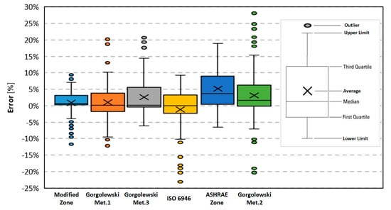
Figure 17.
Statistical box and whisker graph for the evaluated analytical methods.
4. Conclusions
In this work, the accuracy performance of six analytical methods to compute the thermal transmittance (-value) of LSF walls was evaluated. These methods were described and applied to estimate the -values of 80 LSF walls—their precision being evaluated by comparison with the results provided by 2D FEM numerical simulations which were experimentally validated. Trend-lines and respective determination coefficients were obtained for each method. Moreover, the root mean square error (RMSE), the maximum positive error (MaxPE) in absolute and percentage values, as well as the maximum negative error (MaxNE) for each method for all LSF walls were also computed, as well as for each frame type: (1) warm; (2) hybrid; (3) cold. To assess the statistical significance of the obtained analytical percentage -values errors, standard deviations and confidence intervals were computed, and a statistical box and whisker graphs were plotted.
All the evaluated analytical methods showed a quite good accuracy performance, with the RMSE ranging from 0.019 W/(m2·K) up to 0.048 W/(m2·K), or in percentage from 4.1% up to 9.9%. The maximum positive and negative -values errors were +0.156 W/(m2·K) and −0.121 W/(m2·K), respectively. In percentages these error values were +28.1% and −23.1%, respectively.
As expected, given the different LSF walls thermal insulation configuration, the precision of the analytical methods for warm frame walls (RMS errors up to 0.6%, in the ISO 6946 Modified Zone Method) was considerably higher than the one observed on hybrid (RMS errors up to 9.7%, in the ASHRAE Zone Method) and cold frame walls (RMS errors up to 18.4%, in the Gorgolewski Method 2). Moreover, the worst accuracy of the evaluated analytical methods was found in cold frame walls, where all the batt thermal insulation is bridged by the steel studs.
Having taken into account all eighty LSF walls studied alongside the obtained RMS -values errors expressed in percentage, the best accuracy performance was found in the Modified Zone Method (4.1%), while the worst was found in the Gorgolewski Method 2 (9.9%), with the latter also having the higher maximum positive error (+0.156 W/(m2·K); +28.1%), evidencing a tendency to provide conservative -values. The other two Gorgolewski methods (1 and 3) were ranked second (5.8%) and third (6.2%), respectively.
Very surprisingly, since the ISO 6946 standard [20] states that elements where insulation is bridged by metal (e.g., cold and hybrid LSF walls) are out of the scope of this method, the ISO 6946 Combined Method was ranked as the fourth most accurate methodology, exhibiting better performance (7.1%) than other two analytical methods (ASHRAE Zone Method and Gorgolewski Method 2), which were specifically developed for LSF elements. Nevertheless, the use of this analytical method should be performed with some caution, since it was the one that exhibit the larger negative error (−0.121 W/(m2·K); −23.1%), evidencing some trend to provide over-optimistic -values.
Author Contributions
All the authors participated equally to this work. All authors have read and agreed to the published version of the manuscript.
Funding
This research was funded by FEDER funds through the Competitivity Factors Operational Programme—COMPETE and by national funds through FCT—Foundation for Science and Technology within the scope of the project POCI-01-0145-FEDER-032061.

Acknowledgments
The authors also want to thank the support provided by the following companies: Pertecno, Gyptec Ibéria, Volcalis, Sotinco, Kronospan, Hulkseflux, Hilti and Metabo.
Conflicts of Interest
The authors declare no conflict of interest.
Nomenclature
| Symbols | |
| thermal resistance [] | |
| thermal transmittance [] | |
| width of section A (thickness of the steel stud web) [m] | |
| width of section B (wall insulation cavity) [m] | |
| width of section CAV (the remaining wall cavity zone) [m] | |
| layer sheathing thickness [m] | |
| fractional area [---] | |
| flange length [m] | |
| weight factor for the Gorgolewski method [---] | |
| thermal resistivity [] | |
| stud depth [m] | |
| stud spacing [m] | |
| width of section W (steel stud influence zone) [m] | |
| zone factor [---] | |
| thermal conductivity [] | |
| Subscripts | |
| ins | insulation |
| lower | lower limit |
| met | metal |
| n | number of layers or planes |
| q | number of sections or paths |
| se | external surface |
| sheat | sheathing |
| si | internal surface |
| thicker | thicker sheathing side (interior or exterior) |
| tot | total |
| upper | upper limit |
| sections, paths (A, B, C, …) | |
| layers, planes (1, 2, 3, …) | |
| Acronyms | |
| 1D | One-Dimensional |
| 2D | Two-Dimensional |
| 3D | Three-Dimensional |
| AIB | Aerogel Insulation Blanket |
| ASHRAE | American Society of Heating, Refrigerating and Air-conditioning Engineers |
| CBW | Cement Wood Board |
| CHB | Calibrated Hot Box |
| EPS | Expanded Polystyrene |
| ETICS | External Thermal Insulation Composite System |
| FCB | Fibre Cement Board |
| FEM | Finite Element Method |
| GHB | Guarded Hot Box |
| GHP | Guarded Hot Plate |
| GPB | Gypsum Plasterboard |
| GRB | Glassfibre Reinforced Board |
| HB | Hot Box |
| HFM | Heat Flow Meter |
| ICB | Insulation Cork Board |
| IRT | Infrared Thermography |
| ISO | International Standards Organization |
| LSF | Lightweight Steel Frame |
| MaxNE | Maximum Negative Error |
| MaxPE | Maximum Positive Error |
| MW | Mineral Wool |
| OSB | Oriented Strand Board |
| RMSE | Root Mean Square Error |
| TC | Thermocouple |
References
- Santos, P.; da Silva, L.S. Energy Efficiency of Light-Weight Steel-Framed Buildings, 1st ed.; Technical Committee 14—Sustainability & Eco-Efficiency of Steel Construction; European Convention for Constructional Steelwork (ECCS): Mem Martins, Portugal, 2017; ISBN 978-92-9147-105-8. [Google Scholar]
- Soares, N.; Santos, P.; Gervásio, H.; Costa, J.J.; Da Silva, L.S. Energy efficiency and thermal performance of lightweight steel-framed (LSF) construction: A review. Renew. Sustain. Energy Rev. 2017, 78, 194–209. [Google Scholar] [CrossRef]
- Santos, P. Chapter 3—Energy Efficiency of Lightweight Steel-Framed Buildings. In Energy Efficient Buildings; Eng Hwa Yap, Ed.; InTech: London, UK, 2017; pp. 35–60. [Google Scholar]
- Roque, E.; Santos, P.; Pereira, A.C. Thermal and sound insulation of lightweight steel-framed façade walls. Sci. Technol. Built Environ. 2019, 25, 156–176. [Google Scholar] [CrossRef]
- Roque, E.; Santos, P. The Effectiveness of Thermal Insulation in Lightweight Steel-Framed Walls with Respect to Its Position. Buildings 2017, 7, 13. [Google Scholar] [CrossRef]
- Santos, P.; Lemes, G.; Mateus, D. Thermal Transmittance of Internal Partition and External Facade LSF Walls: A Parametric Study. Energies 2019, 12, 2671. [Google Scholar] [CrossRef]
- Soares, N.; Martins, C.; Gonçalves, M.; Santos, P.; da Silva, L.S.; Costa, J.J. Laboratory and in-situ non-destructive methods to evaluate the thermal transmittance and behaviour of walls, windows, and construction elements with innovative materials: A review. Energy Build. 2019, 182, 88–110. [Google Scholar] [CrossRef]
- Gorgolewski, M. Developing a simplified method of calculating U-values in light steel framing. Build. Environ. 2007, 42, 230–236. [Google Scholar] [CrossRef]
- Martins, C.; Santos, P.; da Silva, L.S. Lightweight steel-framed thermal bridges mitigation strategies: A parametric study. J. Build. Phys. 2016, 39, 342–372. [Google Scholar] [CrossRef]
- Santos, P.; Martins, C.; da Silva, L.S.; Bragança, L. Thermal performance of lightweight steel framed wall: The importance of flanking thermal losses. J. Build. Phys. 2014, 38, 81–98. [Google Scholar] [CrossRef]
- Santos, P.; Gonçalves, M.; Martins, C.; Soares, N.; Costa, J.J. Thermal Transmittance of Lightweight Steel Framed Walls: Experimental Versus Numerical and Analytical Approaches. J. Build. Eng. 2019, 25, 100776. [Google Scholar] [CrossRef]
- Sassine, E. A practical method for in-situ thermal characterization of walls. Case Stud. Therm. Eng. 2016, 8, 84–93. [Google Scholar] [CrossRef]
- ISO 9869, Thermal Insulation—Buildins Elements—In-Situ Measurement of Thermal Resistance and Thermal Transmittance—Part 1: Heat Flow Meter Method; ISO—International Organization for Standardization: Geneva, Switzerland, 2014.
- Salmon, D. Thermal conductivity of insulations using guarded hot plates including recent developments and sources of reference materials. Meas. Sci. Technol. 2001, 12, R89. [Google Scholar] [CrossRef]
- ISO 8990, Thermal Insulation—Determination of Steady-State Thermal Transmission Properties—Calibrated and Guarded Hot Box; ISO—International Organization for Standardization: Geneva, Switzerland, 1994.
- Klems, J.H. A calibrated hotbox for testing window systems—Construction, calibration, and measurements on prototype high-performance windows. In Proceedings of the ASHRAE/DOE Conference on the Thermal Performance of the Exterior Envelopes of Buildings, ASHRAE, Orlando, FL, USA, 3–5 December 1979. [Google Scholar]
- Basak, C.K.; Sarkar, G.; Neogi, S. Performance evaluation of material and comparison of different temperature control strategies of a Guarded Hot Box U-value Test Facility. Energy Build. 2015, 105, 258–262. [Google Scholar] [CrossRef]
- Lucchi, E. Applications of the infrared thermography in the energy audit of buildings: A review. Renew. Sustain. Energy Rev. 2018, 82, 3077–3090. [Google Scholar] [CrossRef]
- ASHRAE. Handbook of Fundamentals (SI Edition); ASHRAE—American Society of Heating, Refrigerating and Air-conditioning Engineers: Atlanta, GA, USA, 2017. [Google Scholar]
- ISO 6946, Building Components and Building Elements—Thermal Resistance and Thermal Transmittance—Calculation Methods; ISO—International Organization for Standardization: Geneva, Switzerland, 2017.
- Kosny, J.; Christian, J.E.; Barbour, E.; Goodrow, J. Thermal Performance of Steel-Framed Walls; ORNL report; Oak Ridge National Laboratory: Oak Ridge, TN, USA, 1994. [Google Scholar]
- Kosny, J.; Christian, J.E. Reducing the uncertainties associated with using the ASHRAE zone method for R-value calculations of metal frame walls. In ASHRAE Transactions, Technical and Symposium Papers; Refrigerating and Air-Conditioning Engineers, Inc.: Atlanta, GA, USA, 1995; Volume 101, pp. 779–788. [Google Scholar]
- Doran, S.M.; Gorgolewski, M.T. BRE Digest 465—U-Values for Light Steel-Frame Construction; BRE—Building Research Institute: London, UK, 2002. [Google Scholar]
- THERM. Software Version 7.6.1; Lawrence Berkeley National Laboratory, United States Department of Energy: Berkeley, CA, USA, 2017. Available online: https://windows.lbl.gov/software/therm (accessed on 14 February 2019).
- ISO 10211, Thermal Bridges in Building Construction—Heat Flows and Surface Temperatures—Detailed Calculations; ISO—International Organization for Standardization: Geneva, Switzerland, 2017.
- WeberTherm Uno, Technical Specifications: Weber Saint-Gobain ETICS Finish Mortar. 2018. Available online: https://www.pt.weber/files/pt/2019-04/FichaTecnica_weberthermuno.pdf (accessed on 14 March 2019). (In Portuguese).
- TincoTerm, Technical Sheet: EPS 100. 2015. Available online: http://www.lnec.pt/fotos/editor2/tincoterm-eps-sistema-co-1.pdf (accessed on 14 March 2019). (In Portuguese).
- KronoSpan, Technical Sheet: KronoBuild OSB 3. 2019. Available online: https://de.kronospan-express.com/public/files/downloads/kronobuild/kronobuild-en.pdf (accessed on 14 March 2019).
- Volcalis, Technical Sheet: Alpha Mineral Wool. 2019. Available online: https://www.volcalis.pt/categoria_file_docs/fichatecnica_volcalis_alpharolo-253.pdf (accessed on 14 March 2019). (In Portuguese).
- Santos, C.; Matias, L. ITE50—Coeficientes de Transmissão Térmica de Elementos da Envolvente dos Edifícios; LNEC—Laboratório Nacional de Engenharia Civil: Lisboa, Portugal, 2006. (In Portuguese) [Google Scholar]
- Gyptec Ibérica, Technical Sheet: Standard Gypsum Plasterboard. 2019. Available online: https://www.gyptec.eu/documentos/Ficha_Tecnica_Gyptec_A.pdf (accessed on 14 March 2019). (In Portuguese).
- Pertecno, Catálogo Light Steel Frame. 2015. Available online: http://www.pertecno.pt/pdf/Catálogo-LightSteelFraming.pdf (accessed on 14 March 2019).
- Thermablok, Thermablok® Aerogel Insulation Blanked. 2011. Available online: www.thermablok.co.uk (accessed on 14 March 2019).
- Viroc, Cement Wood Board. 2019. Available online: http://www.viroc.pt/ResourcesUser/Documentos_Viroc/Dossiers_Tecnicos/Viroc_Dossier_Tecnico_PT.pdf (accessed on 14 March 2019).
- Equitone, Fibre Cement Board. 2012. Available online: https://www.equitone.com/pt-pt/materiais/natura/ (accessed on 14 March 2019).
- GRCA. Practical Design Guide for Reinforced Concrete (GRC); GRCA—International Glassfibre Reinforced Concrete Association: Northampton, UK, 2018. [Google Scholar]


© 2020 by the authors. Licensee MDPI, Basel, Switzerland. This article is an open access article distributed under the terms and conditions of the Creative Commons Attribution (CC BY) license (http://creativecommons.org/licenses/by/4.0/).