Hot Blade Shape Reconstruction Considering Variable Stiffness and Unbalanced Load in a Steam Turbine

Abstract

The blades in the low-pressure stage of a steam turbine must be reverse engineered according to the ideal blade shape due to the deformation of the blade during operation. A numerical analysis model of the flow field of the blades is proposed, and the model is solved by alternating between the fluid domain and the solid domain. Considering the imbalance of the load acting on the blade surface and the change in the blade stiffness matrix when the steam turbine is running, the Newton–Raphson method is used to calculate the pressure of the steam fluid on the blade surface and the change in the flow field caused by the blade deformation in each time step. The data are exchanged between the fluid domain and the solid domain after a single-step solution is completed. The simultaneous changes in the fluid domain and the solid domain are discretized in very short time steps, and the process of the blade deformation from stationary to running is simulated by accumulating the time steps. Finally, the trends in the change in the blade deformation and the aerodynamic load during the deformation process are analyzed according to the result of the reconstruction of the blade shape.

1. Introduction

Steam turbines are widely used in power, chemical, and metallurgical industries. When a steam turbine is running, high-temperature and high-pressure steam enters the cylinder through the main valve and the regulating valve, flows through the stator cascades, generates pressure on the surface of the rotor blades, and drives the spindle to rotate, thereby realizing energy conversion and output [1].

A set of blades is known as a stage, and there are many stages in a steam turbine. The blades in each stage are very important for the energy conversion efficiency [2,3], and the influence of the blades in the low-pressure stage on the performance of the steam turbine is particularly significant [4,5,6]. Therefore, the design of the blades has been the focus of research [7].

Based on the research on mathematical modeling [8,9], simulation analysis [10,11], and performance prediction [12,13] of steam turbines, some design methods for the ideal blade shape have been proposed as follows: an eco-design approach for achieving eco-innovative solutions of the turbine blades [7], a reverse-engineering approach of turbine blades for efficiently generating accurate product computer-aided design (CAD) models [14], a modular building block approach for describing the different types of steam turbine blades in detail regarding their geometry and loading [15], a three-dimensional design optimization of steam turbine blades for aerodynamic efficiency enhancement of blades and turbine stages [16], a 3D optimization design method based on an artificial neural network and a genetic algorithm for the rotating blades in a highly loaded turbine [17], and a 3D prescribed surface curvature distribution design method for the high-efficiency turbomachinery blades [18].

In the above-mentioned methods, the ideal blade shape is typically obtained by analyzing the aerodynamic performance according to the designed operating conditions. As steam turbines are operated under conditions such as high loading and high rotational speed, the blades are subjected to multiple complex loads, including centrifugal and aerodynamic loads [4,8,19,20].

The ideal blade shape refers to the ideal shape of the blade to meet the aerodynamic performance requirements of the steam turbine under the designed operating conditions. After the design, the blade shape obtained through manufacturing is called a cold blade shape or a non-running blade shape. The processed blade is subjected to multiple complex loads in a specific operating condition, and the stable state shown by deformation is called a hot blade shape or an operating blade shape. The hot blade shape is the actual shape of the blade under the designed operating conditions. Taking the consistency of hot blade shape and ideal blade shape as the evaluation index, the corresponding cold blade shape is reverse engineered, thereby improving the aerodynamic performance of the steam turbine as much as possible.

In practice, alloy steels are used in blade manufacturing with surface hardening treatment to ensure that the deformation of the blades in running is as small as possible. Although plastic deformation can be controlled to a small range, the elastic deformation still has a significant impact on the design and the analysis of the blade [3,21,22]. Therefore, in the operating conditions, the blade will inevitably deform under the effect of the multiple complex loads, which will cause the blade shape to change and affect the performance of the steam turbine. Therefore, the ideal blade shape cannot be used directly for blade manufacturing. In other words, the “cold” blade shape for manufacturing needs to be reverse engineered according to the ideal blade shape so that the “hot” blade shape formed under the operating conditions is consistent with the ideal blade shape [23,24].

However, the state of the flow field around the blade is closely related to the blade shape and is complex and nonlinear [25,26,27]. Thus, it is difficult to obtain an accurate cold blade shape directly by using the ideal blade shape as the hot blade shape.

Iterative approaches have been proposed for the reverse design of the cold blade shape. First, the initial cold blade shape in the iterative method is obtained based on the ideal blade shape. The ideal blade shape is used as the cold blade shape to estimate the hot blade shape and obtain the deformation, and then the ideal blade shape is reverse deformed to obtain the initial cold blade shape. Second, the reconstruction of the hot blade shape from the cold blade shape and the reverse deformation of the cold blade shape are performed alternately. The cold blade shape is reconstructed in the running state to obtain the hot blade shape, and the accuracy of the cold blade shape is evaluated by comparing the consistency between the hot blade shape and the ideal blade shape. This is an iterative approximation process, and each iteration step includes two parts: reverse deformation and hot reconstruction. The reverse deformation is a simple change of blade shape, which is easy to implement. However, the hot reconstruction is difficult due to the complex load and the deformation of the blade [23].

The fluid–solid coupling method and the fluid–structure interaction method are mainly used in hot blade shape reconstruction to obtain the blade deformation [28,29,30]. Typically, the equilibrium conditions are established based on the ideal blade shape, and the stiffness matrix of the blade no longer changes when the blade displacement is calculated using the finite element method after obtaining the load [31,32,33].

However, due to the variable cross-section and torsional shape of the blades in the low-pressure stage [34], the aerodynamic and the centrifugal loads and the blade stiffness matrix are all functions of the blade shape and will be significantly changed if the blade has a slight shape change.

Therefore, the effect of the variable stiffness of the blade and the unbalanced load in blade deformation should be analyzed to accurately obtain the hot blade shape in the design of steam engine blades [24].

The hot blade shape determines the aerodynamic performance of the steam turbine under the designed operating conditions. The closer the reconstructed hot blade shape from the cold blade shape to the ideal blade shape is, the more reasonable the design of the blade will be. Therefore, the analysis of the reconstructed hot blade shape is of great significance to improve the performance of the steam turbine. In this paper, a simulation model of the blade in the low-pressure stage of a steam turbine is established based on the Newton–Raphson method, which can improve the accuracy of the reconstructed hot blade shape according to the variable stiffness of the blade and the unbalanced aerodynamic load acting on the blade surface. The hot blade shape is reconstructed by a nonlinear finite element method. The differences in shape and aerodynamic load between the hot blade and the ideal blade are compared, and the effects of the reconstruction on blade shape and aerodynamic load are analyzed. Compared with other methods, the proposed method considers the nonlinear effects of the blade structural deformation on aerodynamic analysis, analyzes the variable stiffness of the blade and the unbalanced aerodynamic load during the deformation process, and can effectively improve the accuracy of the reconstructed hot blade shape.

2. Analysis of the Variable Stiffness of the Blades

The centrifugal load caused by the rotor rotation and the aerodynamic load produced by the steam flow cause the change in stiffness of the low-pressure stage blades of a steam turbine, thus the change in stiffness is the key factor affecting the blade deformation. The Newton–Raphson iteration method can be used to accurately calculate the hot blade shape.

The basic equation for nonlinear finite element analysis of the blade is:

$$\mathit{K}\left(\mathit{u}\right)={\mathit{R}}_E$$

(1)

where:

• $\mathit{u}={\left[\begin{array}{cccc}{u}_1& u_2& \cdots & u_n\end{array}\right]}^{\mathrm{T}}$ is the displacement vector of a blade node;
• $\mathit{K}\left(\mathit{u}\right)={\left[\begin{array}{cccc}{K}_1\left(\mathit{u}\right)& K_2\left(\mathit{u}\right)& \cdots & K_n\left(\mathit{u}\right)\end{array}\right]}^{\mathrm{T}}$ is the nonlinear internal force vector of $\mathit{u}$; and
• ${\mathit{R}}_E={\left[\begin{array}{cccc}{R}_1& R_2& \cdots & R_n\end{array}\right]}^{\mathrm{T}}$ is an external force vector.

The Newton–Raphson method starts with a hypothetical solution and gradually increases the approximation of the solution by iteration until the solution satisfies the preset convergence condition. If the approximate solution of the blade shape in the $i$-th iteration step is ${\mathit{u}}^i$, the first-order Taylor expansion of the approximate solution in the next iteration step can be expressed as:

$$\mathit{K}\left({\mathit{u}}^{i+1}\right)\approx \mathit{K}\left({\mathit{u}}^i\right)+{\mathit{K}}_{\mathit{T}}^{\mathit{i}}\Delta {\mathit{u}}^i={\mathit{R}}_E\Rightarrow {\mathit{K}}_{\mathit{T}}^{\mathit{i}}\Delta {\mathit{u}}^i={\mathit{R}}_E-\mathit{K}\left({\mathit{u}}^i\right)$$

(2)

where $\Delta {\mathit{u}}^i$ is the increment of the node displacement and ${\mathit{K}}_{\mathit{T}}^{\mathit{i}}={\left(\partial \mathit{K}/\partial \mathit{u}\right)}^{\mathit{i}}$ is the tangential stiffness matrix of the $i$-th iteration step, indicating the nonlinear stiffness of the blade, i.e.:

$${\mathit{K}}_{\mathit{T}}^{\mathit{i}}=\left[\begin{array}{cccc}\frac{\partial {\mathit{K}}_1\left({\mathit{u}}^i\right)}{\partial u_1}& \frac{\partial {\mathit{K}}_1\left({\mathit{u}}^i\right)}{\partial u_2}& \cdots & \frac{\partial {\mathit{K}}_1\left({\mathit{u}}^i\right)}{\partial u_n}\\ \frac{\partial {\mathit{K}}_2\left({\mathit{u}}^i\right)}{\partial u_1}& \frac{\partial {\mathit{K}}_2\left({\mathit{u}}^i\right)}{\partial u_2}& \cdots & \frac{\partial {\mathit{K}}_2\left({\mathit{u}}^i\right)}{\partial u_n}\\ ⋮& ⋮& & ⋮\\ \frac{\partial {\mathit{K}}_n\left({\mathit{u}}^i\right)}{\partial u_1}& \frac{\partial {\mathit{K}}_n\left({\mathit{u}}^i\right)}{\partial u_2}& \cdots & \frac{\partial {\mathit{K}}_n\left({\mathit{u}}^i\right)}{\partial u_n}\end{array}\right],\Delta {\mathit{u}}^i=\left[\begin{array}{c}\Delta {\mathit{u}}_1\\ \Delta {\mathit{u}}_2\\ ⋮\\ \Delta {\mathit{u}}_n\end{array}\right]$$

(3)

The resulting linearization equation is:

$${\mathit{K}}_{\mathit{T}}^{\mathit{i}}\Delta {\mathit{u}}^i={\mathit{R}}^i$$

(4)

where ${\mathit{R}}^i$ is the unbalanced force vector and ${\mathit{R}}^i={\mathit{R}}_E-{\mathit{R}}_I^i$ with ${\mathit{R}}_E$ including all external loads such as centrifugal load and aerodynamic load, ${\mathit{R}}_I^i$ being the internal force vector, and ${\mathit{R}}_I^i=\mathit{K}\left({\mathit{u}}^i\right)$. The displacement increment $\Delta {\mathit{u}}^i$ of the blade shape is obtained by solving Equation (4), and the new approximate solution is:

$${\mathit{u}}^{i+1}={\mathit{u}}^i+\Delta {\mathit{u}}^i$$

(5)

The residual of this equation is:

$${\mathit{R}}^{i+1}={\mathit{R}}_E-\mathit{K}\left({\mathit{u}}^{i+1}\right)={\mathit{R}}_E-{\mathit{R}}_I^{i+1}\ne 0$$

(6)

If ${\mathit{R}}^{i+1}$ is small enough, $u^{i+1}$ can be considered a satisfactory solution, and ${\mathit{K}}_{\mathit{T}}^{\mathit{i}+\mathbf{1}}$ is the blade stiffness in this state. Otherwise, let:

$${\mathit{u}}^i={\mathit{u}}^{i+1}$$

(7)

$$\Delta {\mathit{u}}^i=\Delta {\mathit{u}}^{i+1}$$

(8)

$${\mathit{R}}_I^i={\mathit{R}}_I^{i+1}$$

(9)

And continue the iterative solution process until the residual converges to the termination condition of the iteration, which is expressed in the following normalized form:

$$\epsilon =\frac{{\Vert {\mathit{R}}^{i+1}\Vert }^2}{1+{\Vert {\mathit{R}}_E\Vert }^2}=\frac{{{\displaystyle \sum }}_{j=1}^n{\left({\mathit{R}}_j^{i+1}\right)}^2}{1+{{\displaystyle \sum }}_{j=1}^n{\left({\mathit{R}}_{Ej}\right)}^2}\le \left[\epsilon \right]$$

(10)

The process of solving the above-mentioned nonlinear variable stiffness static equation based on the Newton–Raphson iteration method to obtain the blade stiffness is shown in Figure 1.

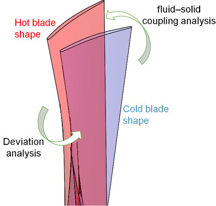
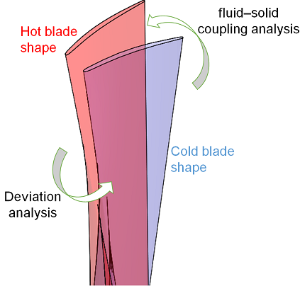
3. Hot Blade Shape Reconstruction Under an Unbalanced Load

Considering the variable stiffness of the blade and the unbalanced load acting on the blade surface, the blade stiffness and the load conditions must be updated while the blade shape changes during the reconstruction of the hot blade shape. The fluid–structure interaction analysis method based on a three-dimensional nonlinear Navier–Stokes computational fluid dynamics (CFD) solver and a structural mechanics finite element solver is used to establish a Newton–Raphson iterative process with alternating solutions and data exchange. The solution process begins with a cold blade shape, and the relationship between the cold blade shape ${\mathit{u}}_{cold}$ and the hot blade shape ${\mathit{u}}_{hot}$ is as follows:

$${\mathit{u}}_{hot}={\mathit{u}}_{cold}+\Delta \mathit{u}$$

(11)

Equation (11) is the basis of the hot blade shape reconstruction.

The detailed steps are as follows:

• The CFD solver is used to simulate the flow field around the cold blade under the preset boundary conditions to obtain the aerodynamic load acting on the blade surface.
• The external force vector ${\mathit{R}}_{\mathit{E}}^{\mathit{i}}$ under the action of the aerodynamic and the centrifugal loads and the internal force vector $R_I^i$ in its current state based on the variable stiffness analysis of the blade are calculated to obtain the unbalanced load $R_I^i$. The deformation $\Delta {\mathit{u}}^i$ of the current cold blade is then calculated using a structural mechanics solver.
• The deformation of the cold blade $\Delta {\mathit{u}}^i$ is transmitted to the fluid mesh, which is updated by the dynamic mesh technique, and the CFD solver is used again to simulate the flow field around the cold blade under the set boundary conditions to obtain the aerodynamic load acting on the blade surface corresponding to the current blade shape.
• If the difference of the aerodynamic load data from step (1) and step (3) meets the convergence condition of the CFD solver, the analysis process is ended, and the structural mechanics solver is used to obtain the deformation of the cold blade $\Delta {\mathit{u}}^i$ based on the aerodynamic load in the current state. Otherwise, the analysis of the cold blade deformation is continued from step (2).
• $\Delta {\mathit{u}}^i$ is used as the hypothetical solution to modify the cold blade shape ${\mathit{u}}_{cold}$ and obtain the hot blade ${\mathit{u}}_{hot}^i$, which is simulated using the CFD solver to obtain the corresponding aerodynamic load.
• Steps (2) and (3) are executed again to obtain the deformation $\Delta {\mathit{u}}^{i+1}$ of the current hot blade and the corresponding aerodynamic load.
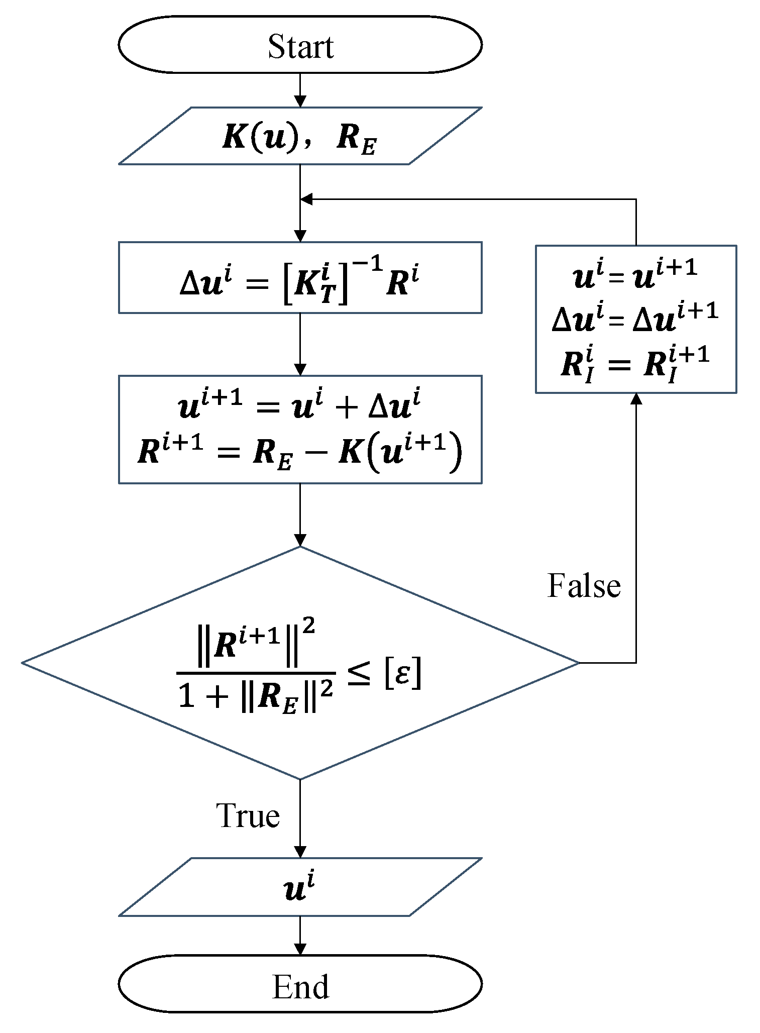
• The external force vector ${\mathit{R}}_{\mathit{E}}^{\mathit{i}+\mathbf{1}}$ and the internal force vector $R_I^{i+1}$ of the blade in its current state are calculated according to the aerodynamic and the centrifugal loads to determine whether the convergence conditions of the Newton–Raphson iteration method are met. If they are, it can be considered that the state of the hot blade shape is no longer changed, and the solution process ends. Otherwise, the process is performed again from step (5).

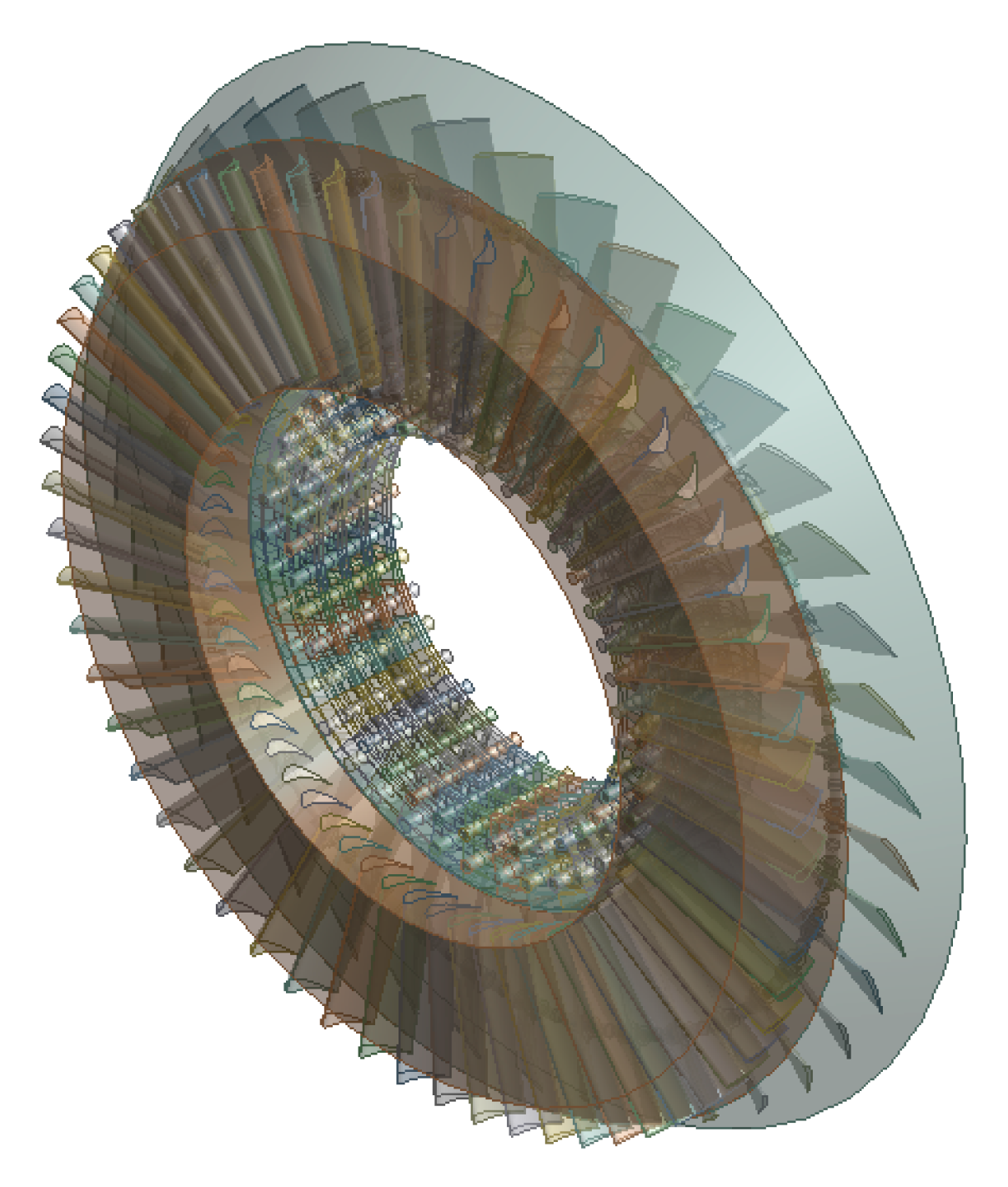
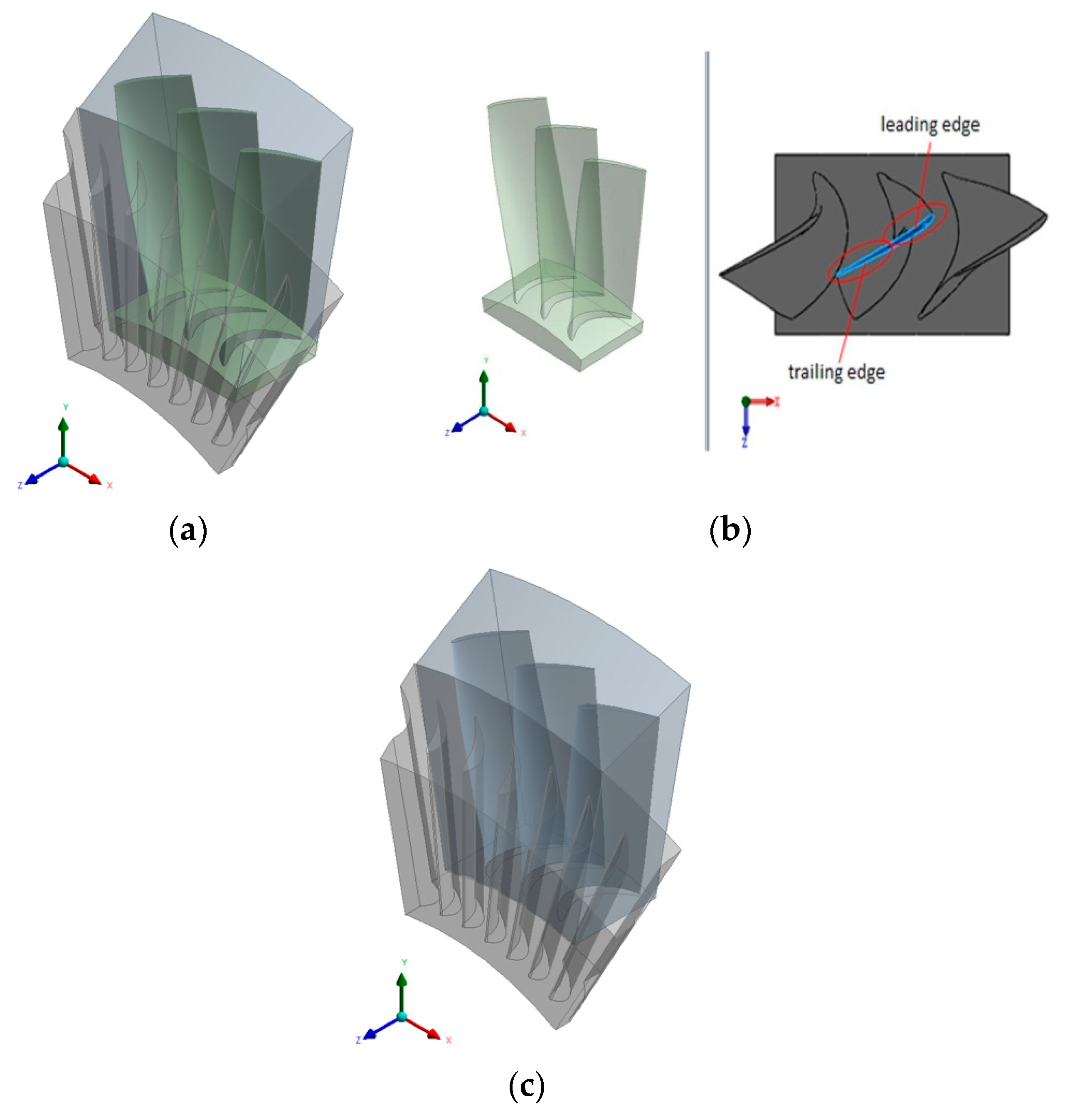
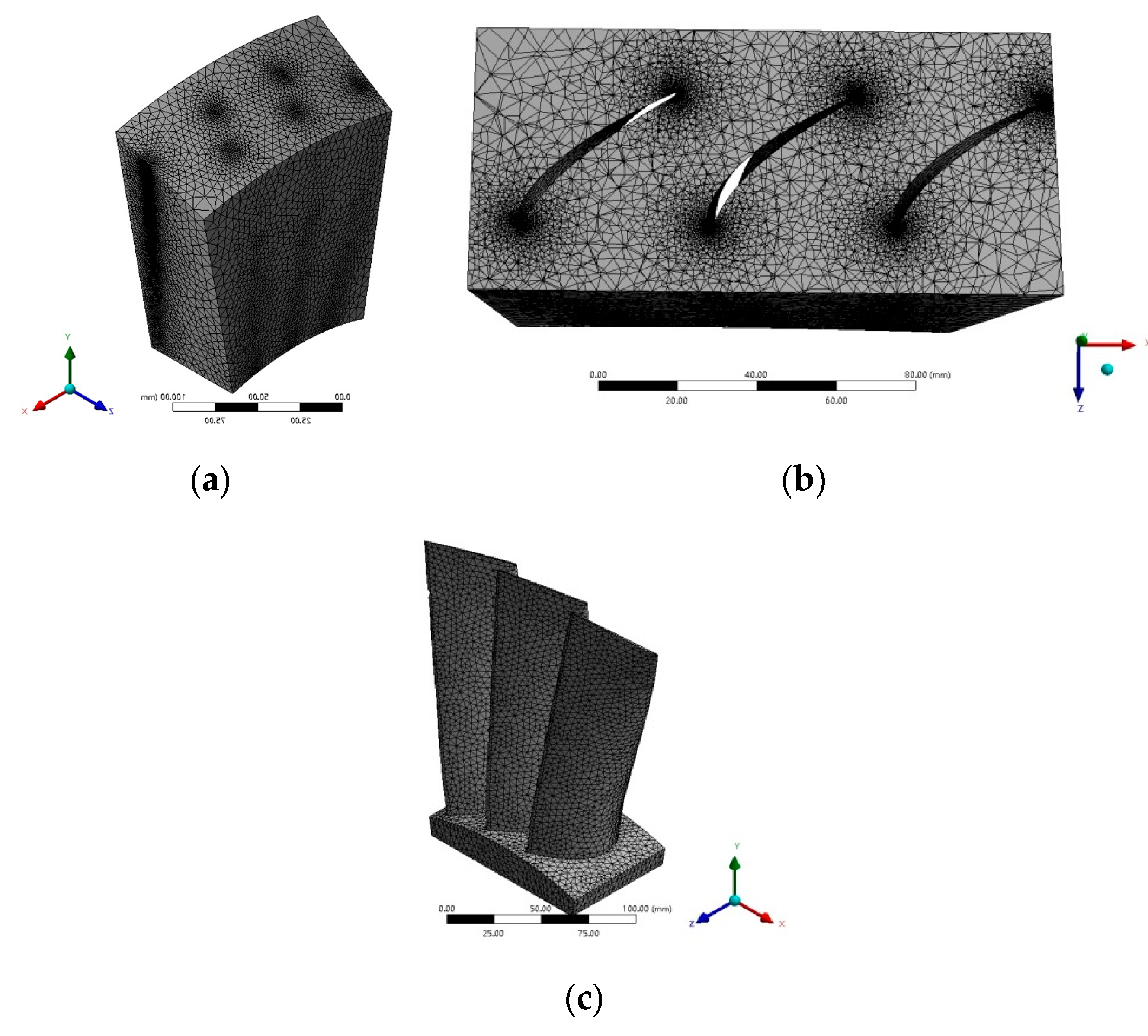
4. Simulation Model of Hot Blade Shape Reconstruction

The steam flow in the low pressure stage of a steam turbine is not uniform along the axial direction due to the influence of the stator blades. Therefore, the influence of stator blades on the flow field should be considered in the analysis of the rotor blades. According to the assembly model of the stator and the rotor blades, Boolean operations are performed on the fluid region and the solid region to obtain a full-circle model of the low pressure stage containing both the blade model and the flow field model, as shown in Figure 2.

Considering the extensive calculation requirements of the analysis of the flow field of the full-circle model and the periodic distribution of blades in the circumference direction, only a single blade is needed for numerical analysis. The calculation data can be mapped and transmitted between the boundaries on both sides of the selected blade model by setting periodic boundaries. A fixed rotor model with good robustness and low consumption of computing resources is used to express the interface between the fluid regions of the stator blades and the rotor blades. In addition, a method of changing the reference coordinate system while maintaining the relative position of the components is used to handle the flow from one component to the next, thus the analysis result of a single blade is consistent with that of all the blades while reducing the analysis range.

Making the transition from all the blades to a single blade, the analysis area needs to be divided, and the boundary of the flow field around a single blade will affect the accuracy of the numerical analysis results. The flow field of a rotor blade is continuous between its two adjacent rotor blades, and the accurate calculation of the flow state of steam in this area is the basis for obtaining the aerodynamic load acting on the blade surface. Therefore, the analysis model of the rotor blade is established with a single rotor blade as the main object, and the flow field is extended to its adjacent blades. At the same time, a set of stator blades is selected as auxiliary objects to cause the output steam flow from the stator blades to completely cover the flow field on both sides the rotor blade. In this way, the divided analysis model can be as close as possible to the flow field around the rotor blade during the actual operation of the steam turbine.

Because the analysis focuses on the blade deformation caused by the pressure of the flow field around the blade, a 3D analysis model that includes only the working part of the blade is established, as shown in Figure 3. The model rotates around the Z axis, and the Y and the X axes correspond to the radial and the tangential directions, respectively.

Unstructured meshes are more suitable for meshing objects with complex curved surfaces and rapid editing of mesh nodes than are structured meshes, thus unstructured tetrahedral meshes are used to mesh the flow field on the complex surface of the rotor blade. The mesh of the flow field model and the mesh of the blade model are shown in Figure 4.

ANSYS CFX and the IAPWS-IF97 STREAM 5V steam model [35] are selected for a CFD analysis of the low pressure stage of the steam turbine under the following conditions:

• Inlet pressure: 49.25 kPa;
• Temperature: 348.27 K;
• Outlet pressure: 0.0135 MPa;
• Blade material: 2Cr13;
• Material density: 7750 kg/m³;
• Young’s modulus: 2.19 × 10⁵MPa;
• Poisson’s ratio: 0.315;
• Yield strength: 440 MPa;
• Tensile strength: 655 MPa.

The settings of CFD analysis is shown in

Table 1. Settings of computational fluid dynamics (CFD) analysis.

Solver	Type	Pressure-Based
	Velocity Formulation	Absolute
	Time	Steady
Model	Viscous	Renormalization-group (RNG) k-epsilon, Standard Wall Functions
Solution Methods	Pressure-Velocity Coupling Scheme	Simple
	Spatial Discretization	Gradient	Least Squares Cell Based
		Pressure	PRESTO!
		Momentum	Second Order Upwind
		Volume Fraction	First Order Upwind
		Turbulent Kinetic Energy	First Order Upwind
Solution Controls	Under-Relaxation Factors	Pressure	0.3
		Density	1
		Body Forces	1
		Momentum	0.7
		Volume Fraction	0.5

.

In addition, the three-dimensional nonlinear Navier–Stokes computational fluid dynamics (CFD) solver and the structural mechanics finite element solver are used to execute the analysis. The two solvers are used to establish a Newton–Raphson iterative process with alternating solutions and data exchange.

5. Analysis of the Simulation Results of Hot Blade Shape Reconstruction

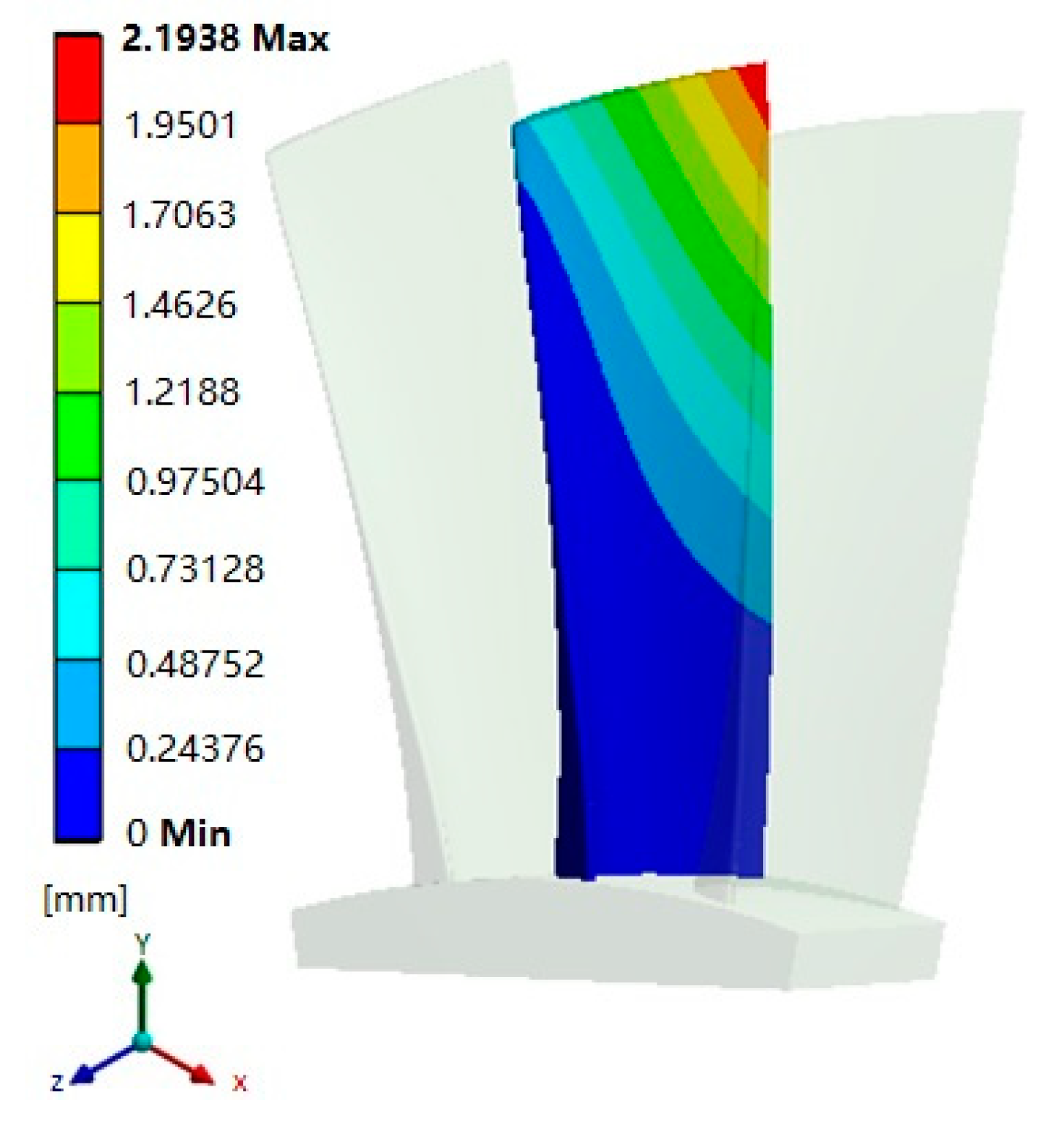
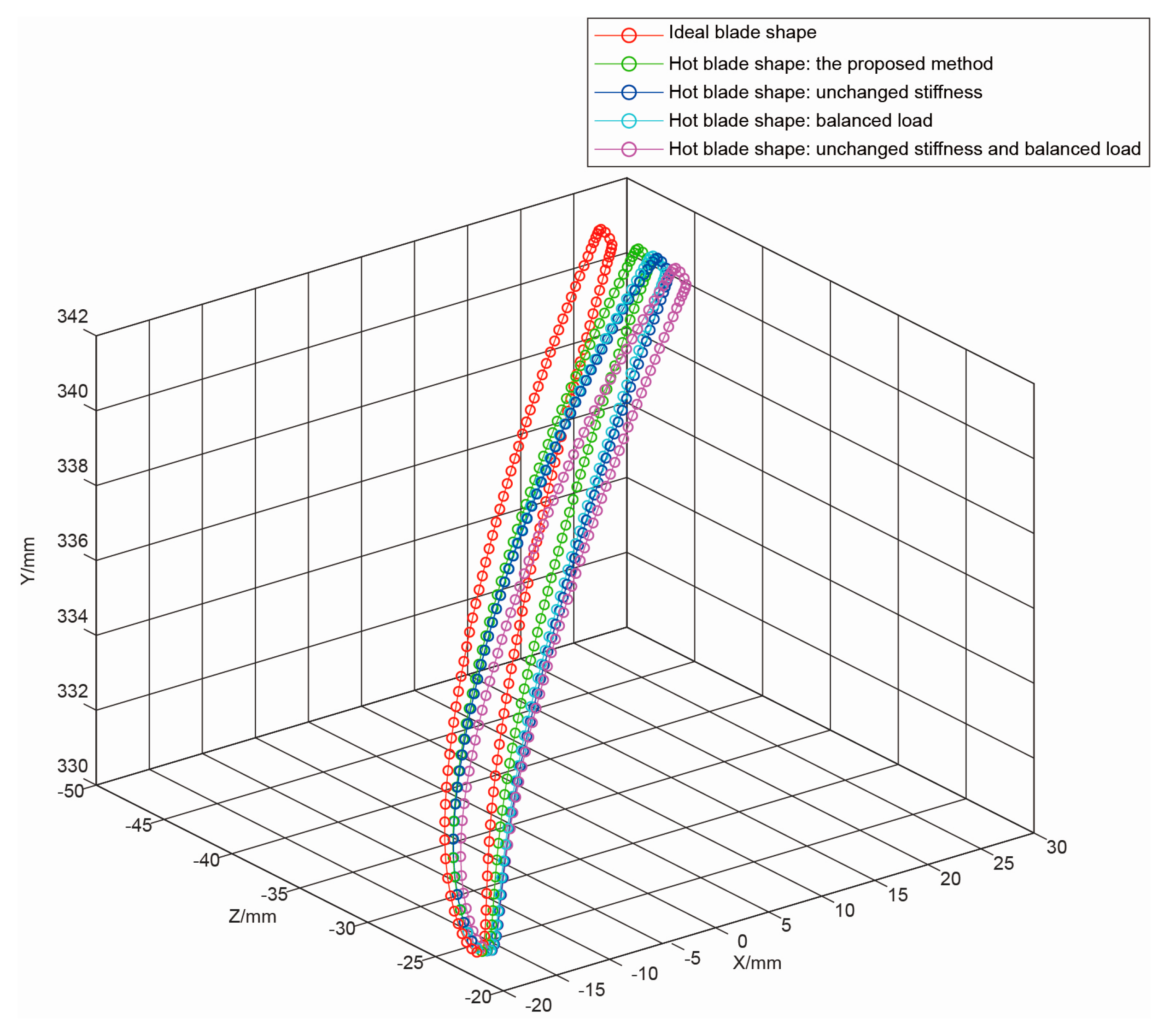
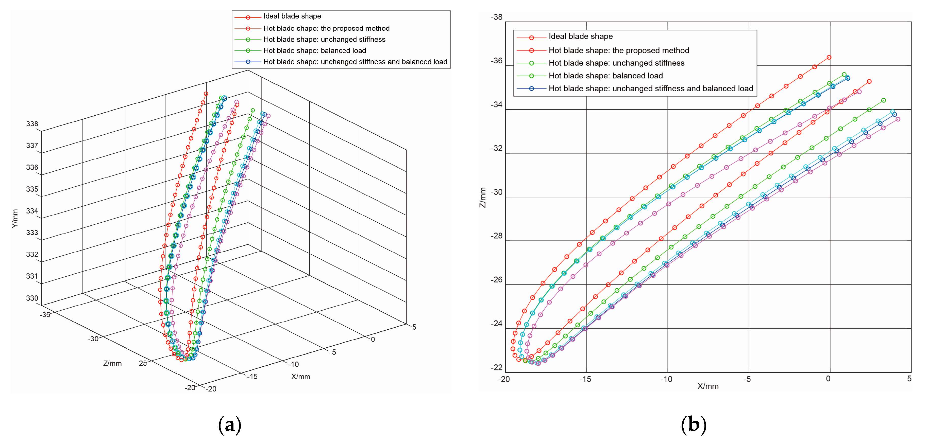
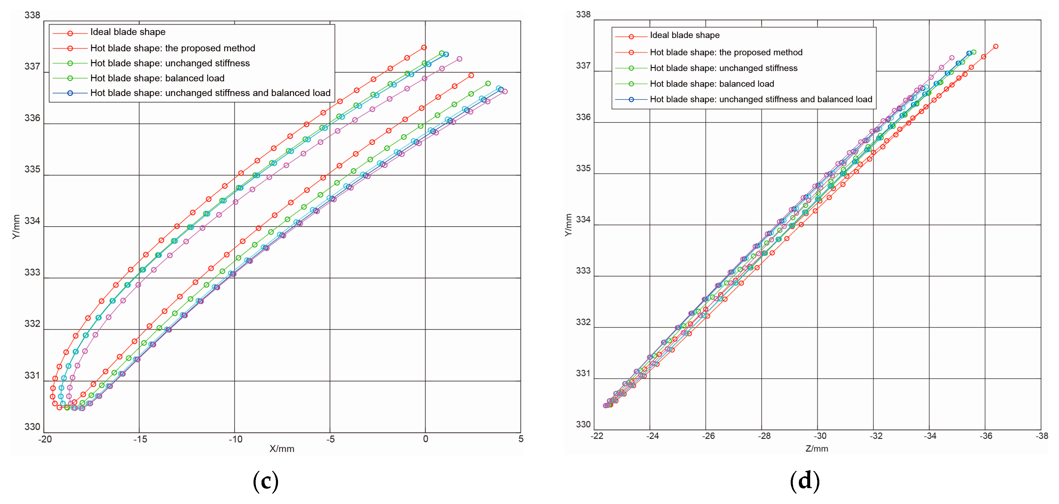
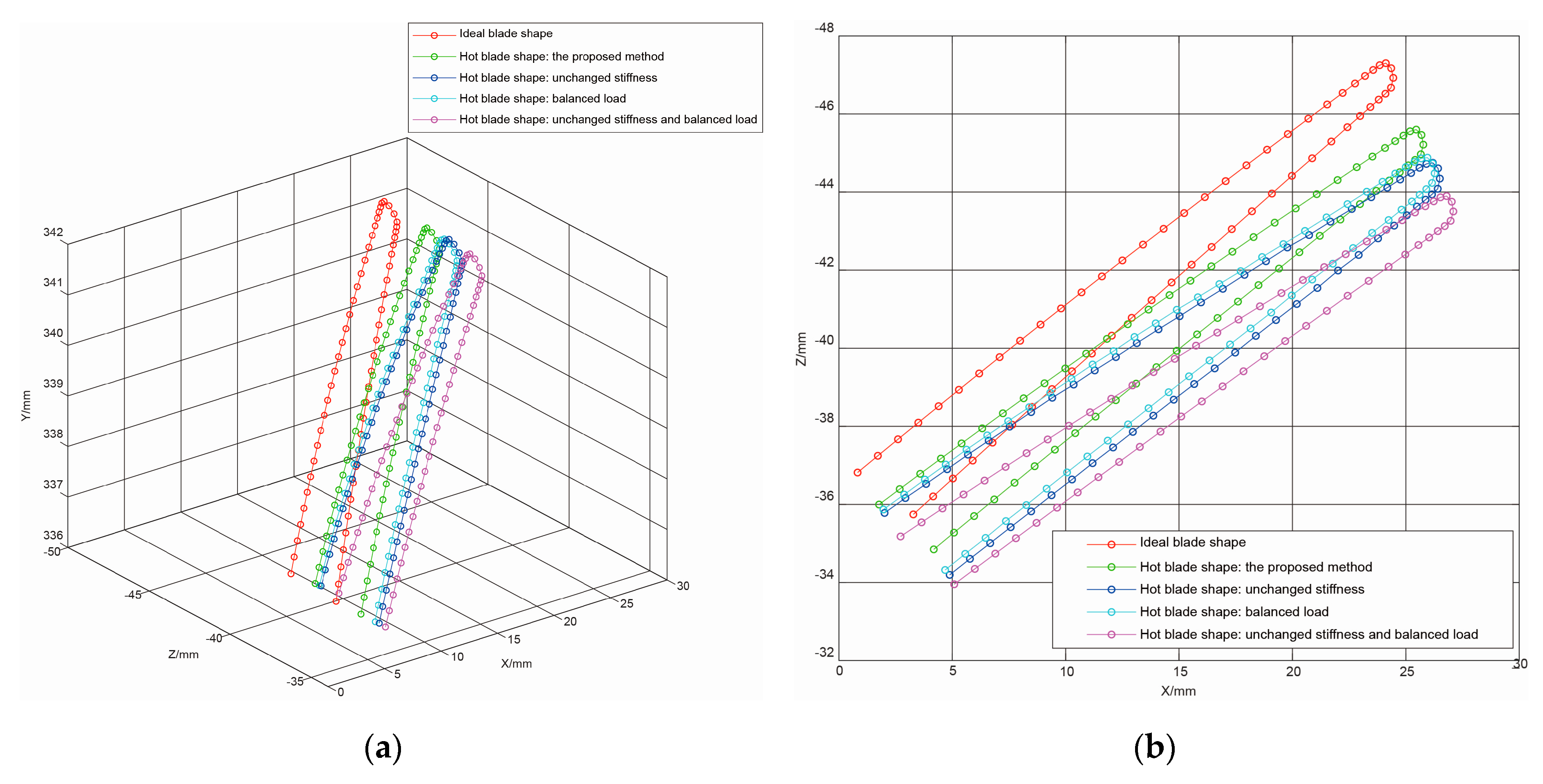
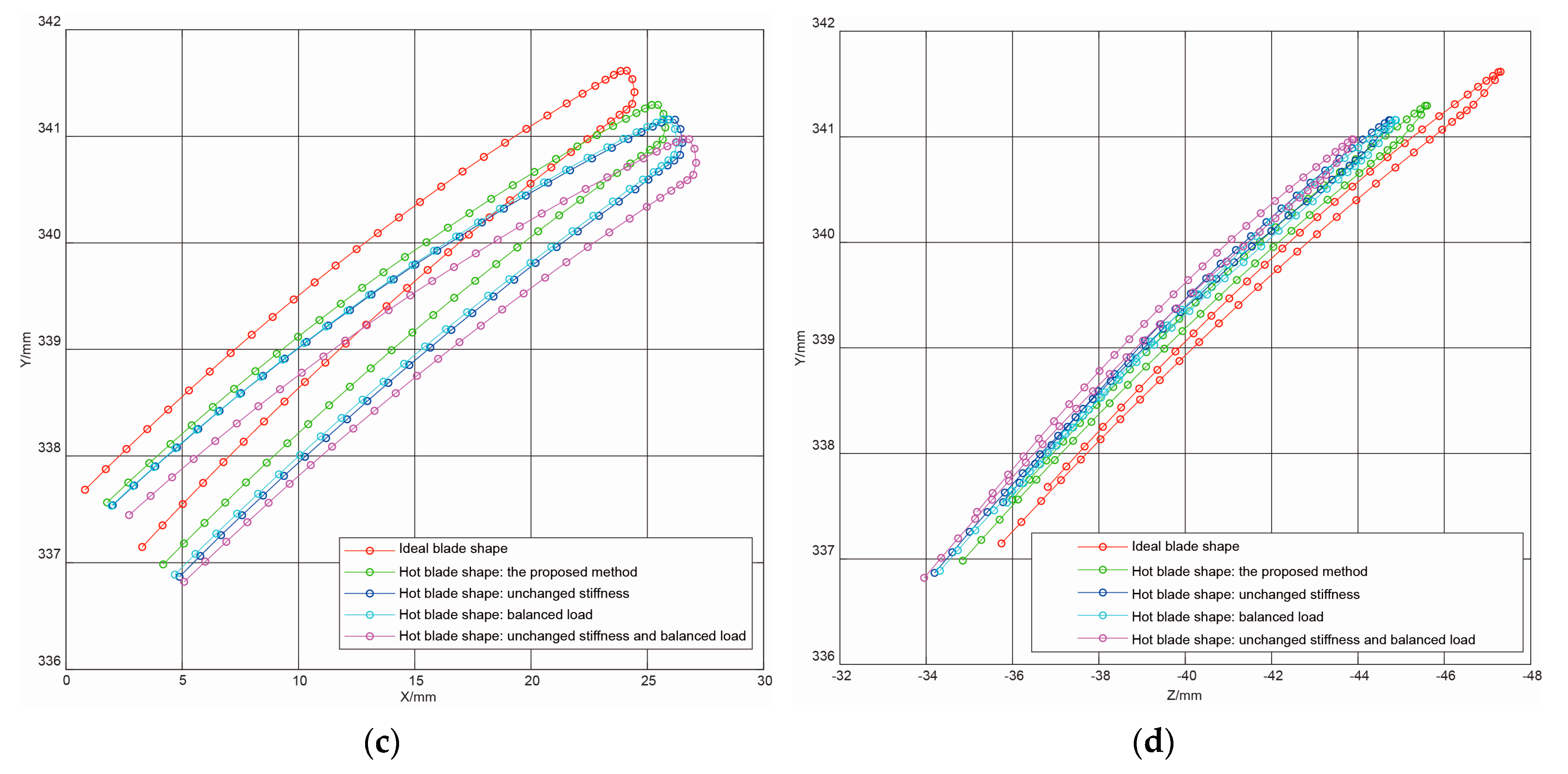
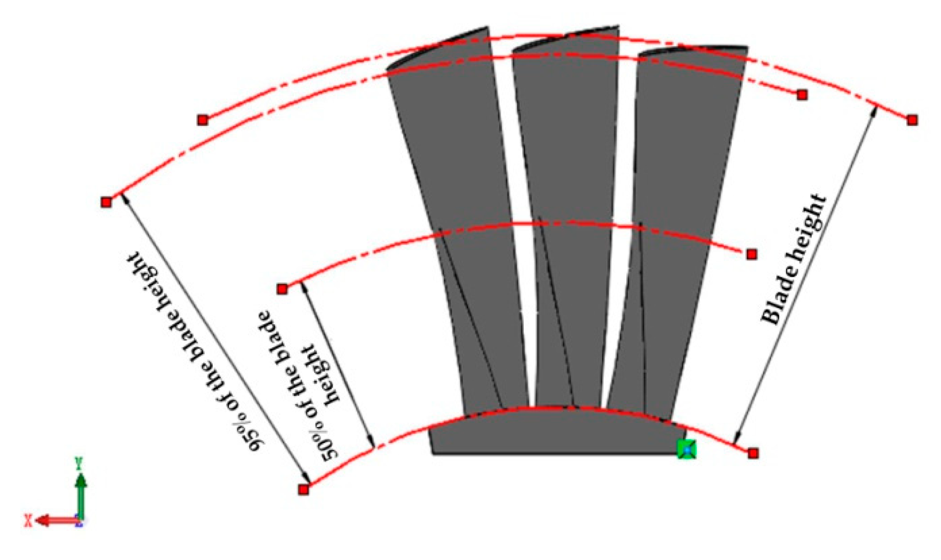
5.1. Deviation of the Reconstructed Blade Shape

The total deformation of the blade under centrifugal and aerodynamic loads is shown in Figure 5.

Simulation results show that the deformation of the hot blade is mainly in the upper part. That is, the blade gradually deviates from the ideal shape from the middle to the top, and the maximum is at the trailing edge of the blade top. The contour line at the blade top is selected to analyze the shape change trend under multiple loads, and the coordinate changes of the corresponding nodes before and after the change of the ideal shape are compared, as shown in Figure 6.

Compared with the methods that did not consider the variability of stiffness of the blade and the unbalanced load acting on the blade surface, the reconstructed hot blade shape obtained by our proposed method is closer to the ideal blade shape. Therefore, our proposed method can effectively improve the accuracy of the reconstructed hot blade shape and is verified to be effective.

The displacement of the nodes of the contour line shows that the blade deformation is mainly the twist of the blade in its rotation direction and that the difference in deformation between the leading and the trailing edges of the blade top is significant.

The positions of the nodes at the leading edge of the blade top before and after the deviation are shown in Figure 7.

Figure 7 shows that the deviation of the leading edge node of the blade top during the hot blade shape reconstruction is small and that the minimum is at the leading edge vertex. The components of the deviation of the nodes in the axial and the tangential directions are larger, and the component in the radial direction is smaller.

The deformation is mainly at the trailing edge of the upper half of the blade, and the maximum is at the trailing edge of the top. Therefore, the deviation trend of the nodes at the trailing edge contour line represents the deformation trend of the blade in hot blade shape reconstruction.

The positions of the nodes at the trailing edge of the blade top before and after the deviation are shown in Figure 8.

Figure 8 shows that the trailing edge of the blade top is mainly deflected backward in the direction of rotation of the blade, and the nodes near the trailing edge have a larger deviation. The components of the deviation of the nodes in the tangential direction are larger, and the component in the radial direction is smaller, which indicates that the main deformation of the trailing edge of the blade top under multiple loads is torsion without obvious stretching.

The analysis of the positional displacement of the leading and the trailing edges of the blade top shows that the blade deformation under multiple loads in hot blade shape reconstruction increases along the direction of the blade height. The analysis of the deviation of the nodes at the leading and the trailing edges of the blade top shows that the blade shape will be twisted under the multiple loads in hot blade shape reconstruction. The elongation of the blade in the radial direction is very small, and the deviation of the leading edge is also small. The main deformation of the blade is the axial and the tangential deflection of the trailing edge in the direction of rotation, and the deviation increases in the direction of the blade height.

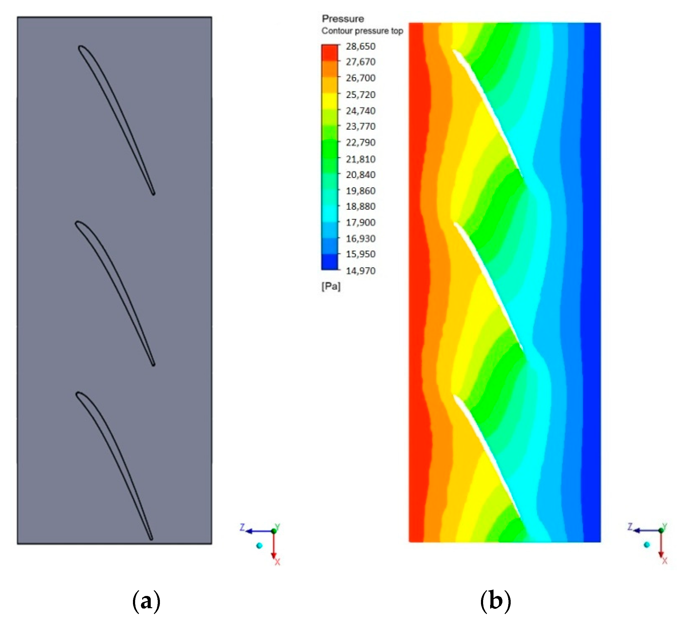
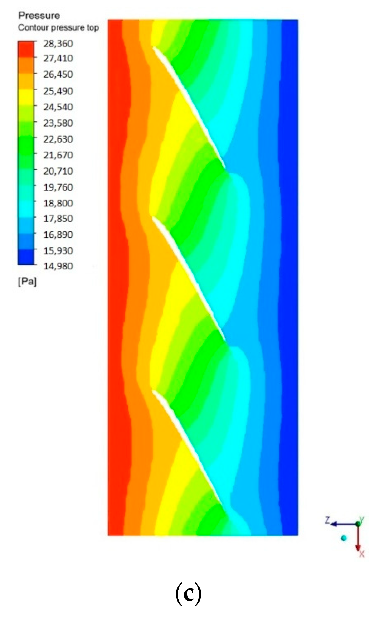
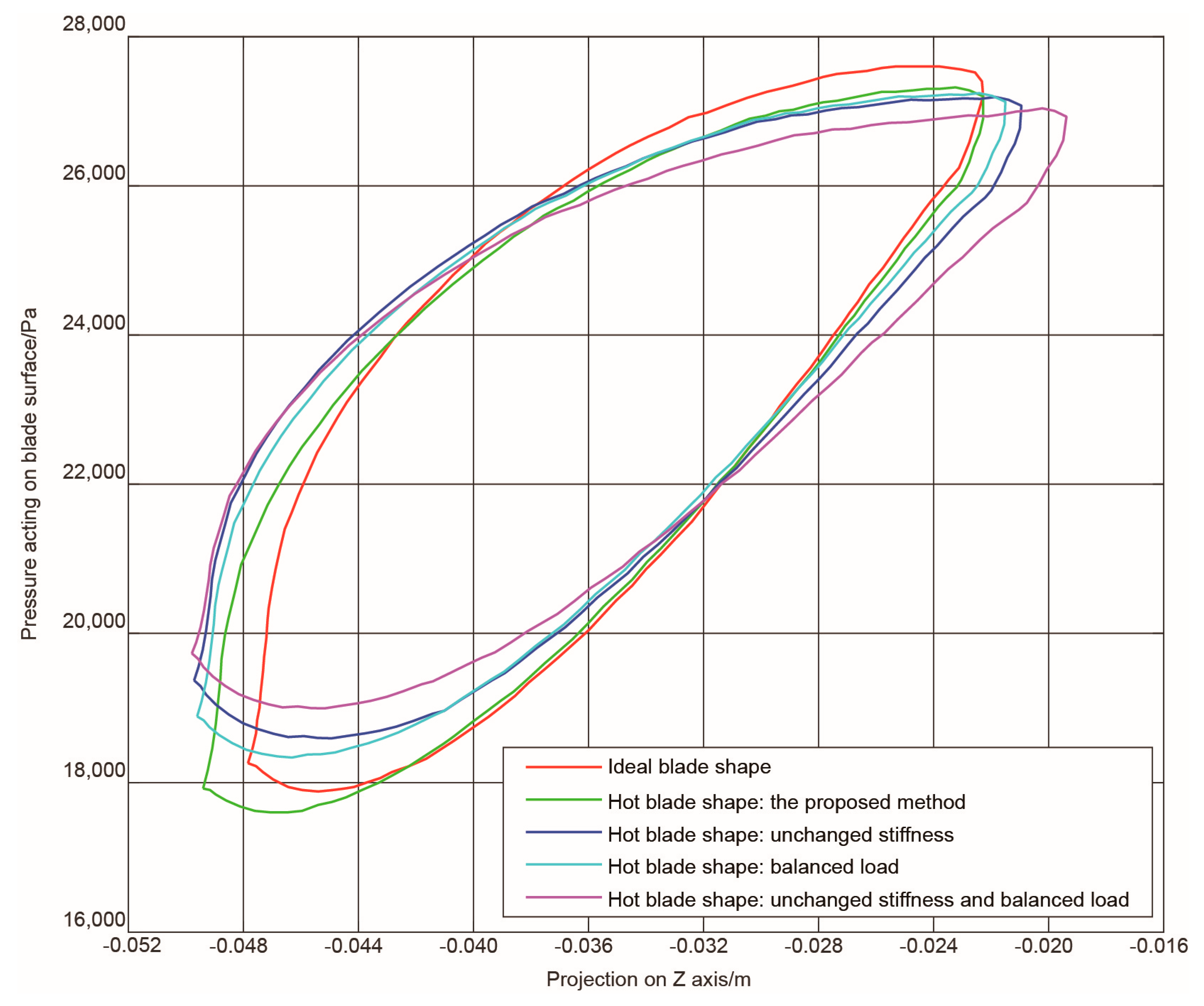
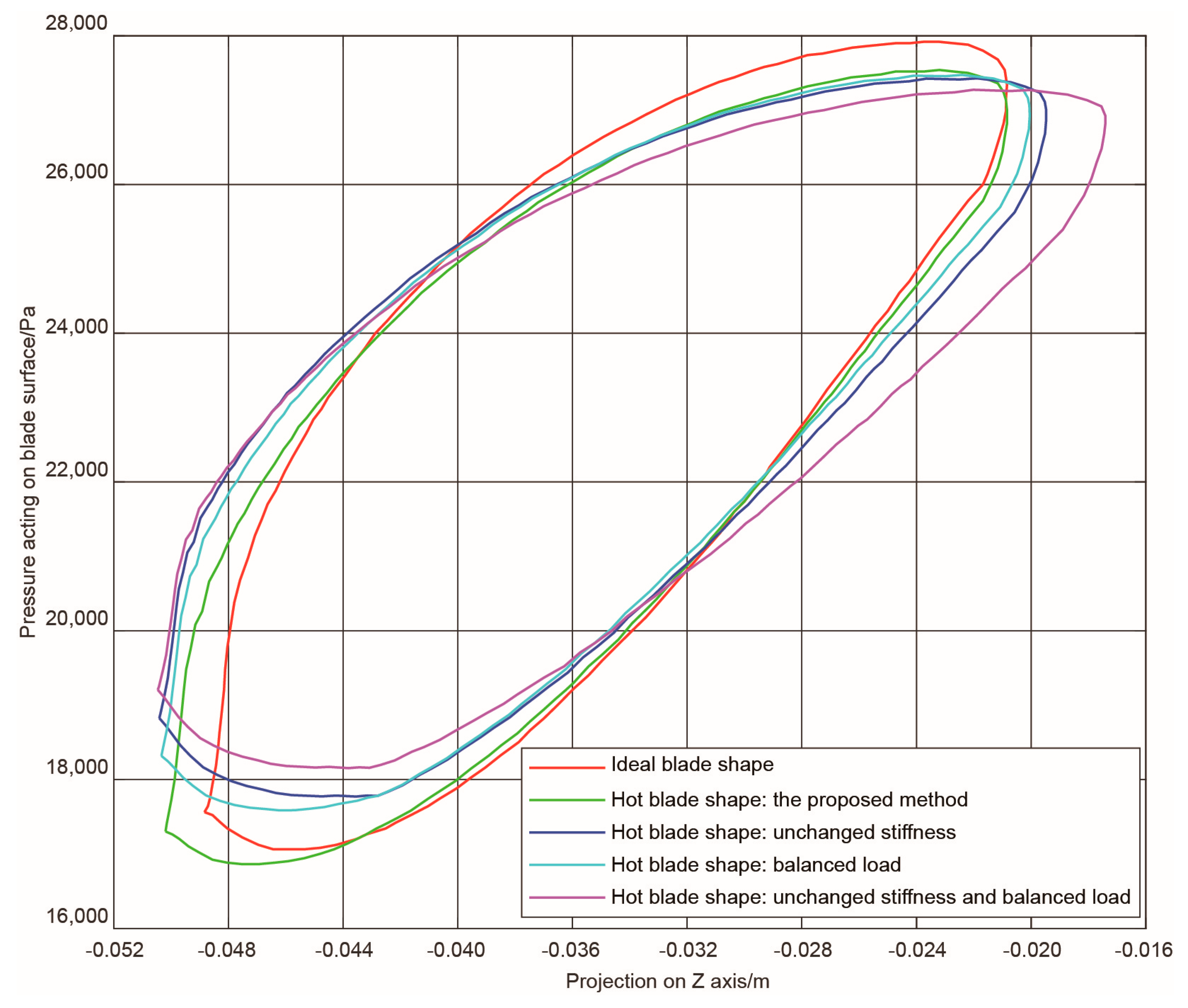
5.2. Changes in Aerodynamic Loads on the Hot Blade

In hot blade shape reconstruction, the change in blade shape directly affects the flow field around the blade, thus the direction, the distribution, and the value of the aerodynamic load on the blade surface will change accordingly.

Therefore, the Newton–Raphson iteration method is used to calculate the blade deformation under the combined action of centrifugal and aerodynamic loads, and both the steam pressure data and the blade displacement data are transferred between each time step to obtain accurate aerodynamic load data.

Two representative heights on the upper half of the blade are selected to analyze the difference in the aerodynamic load between the ideal blade shape and the hot blade shape. They are shown in Figure 9.

Since the deformation at the blade top is the largest, the steam pressure acting here can clearly reflect the change of the aerodynamic load in the reconstruction of the hot blade shape. Considering the difference in the height of the leading and the trailing edges of the blade top, the steam pressure at 95% of the blade height is selected for analysis. A comparison of the steam pressure distribution shows in Figure 10 the difference in steam flow between the hot blade shape and the ideal blade shape.

Figure 10 shows that the steam pressure distribution corresponding to the hot blade shape and the ideal blade shape are substantially the same. However, a significant difference is that the steam pressure at the trailing edge of the suction side of the hot blade shape is lower than that of the ideal blade shape. To compare the differences in the steam pressure on the blade surface in detail, the pressure at each point of the cross-sectional profile at 95% of the blade height is selected and arranged according to the Z axis coordinate. The cross-sectional profile is shown in Figure 11. The resulting pressure curves are shown in Figure 12.

The comparison of the pressure curves in Figure 12 shows that the deformation of the blade under multiple loads reduces the pressure in the upstream region of the pressure surface and increases the pressure in the downstream region. The deformation also makes the projection of the trailing edge of the blade at the same height longer in the axial direction, which in turn makes the pressure at the trailing edge of the suction surface smaller.

Since the deformation is mainly in the upper half of the blade, a comparison of the pressure acting on the blade surface at 50% of the blade height can be used to reveal the trend of the difference in aerodynamic load when the blade deformation is reduced. The pressure curves are shown in Figure 13.

The comparison of the pressure curves in Figure 13 shows that the difference between the pressure curves decreases due to the reduction of the blade deformation, which is still similar to the situation at 95% blade height. However, the pressure curves at the trailing edge are closer due to the reduction in the deviation, thus the range between the lower steam pressure on the pressure surface of the hot blade and the higher steam pressure on the ideal blade is increased; additionally, the difference in the steam pressure distribution between the suction surfaces of the two blades is small.

The above-mentioned analysis of hot blade shape reconstruction shows that the change in steam pressure causes the coupling between blade deformation and the nonlinear aerodynamic load to be closer. The torsional deformation of the blade increases the flow area and the flow ratio, increases the radial and the lateral steam loss, and changes the pressure gradient of the steam flow along the blade height.

In addition, the comparison of the pressure curves in Figure 12 and Figure 13 shows that the aerodynamic load acting on the blade obtained by our proposed method is closer to the actual situation compared with the methods that did not consider the variability of stiffness of the blade and the unbalanced load acting on the blade surface. Therefore, it can effectively provide a more reasonable data basis for further blade design and analysis.

6. Conclusions

In this paper, the variable stiffness of the low pressure stage blades of steam turbines and the unbalanced aerodynamic load on the blade surfaces were analyzed. The Newton–Raphson method was used to establish a simulation model of the blade in the actual working space. The nonlinear finite element method was used for simulation analysis, and hot blade shape reconstruction in the design process was realized.

The results of the analysis show that the main deformation of the hot blade is the twist of the trailing edge at the top of the blade in the direction of rotation, and the variation in the aerodynamic load is related to the increase in the pressure acting on the pressure surface near the trailing edge, while the pressure acting on the suction surface near the trailing edge decreases.

References

1. Sarkar, D.K. Steam Turbines. In Thermal Power Plant; Sarkar, D.K., Ed.; Elsevier: Amsterdam, The Netherlands, 2015; pp. 189–237. [Google Scholar] [CrossRef]
2. Prabhunandan, G.S.; Byregowda, H.V. Dynamic Analysis of a Steam Turbine with Numerical Approach. Mater. Today-Proc. 2018, 5, 5414–5420. [Google Scholar] [CrossRef]
3. Lucacci, G. Steels and alloys for turbine blades in ultra-supercritical power plants. In Materials for Ultra-Supercritical and Advanced Ultra-Supercritical Power Plants; Di Gianfrancesco, A., Ed.; Woodhead Publishing: Cambridge, UK, 2017; pp. 175–196. [Google Scholar]
4. Tanuma, T. Development of last-stage long blades for steam turbines. In Advances in Steam Turbines for Modern Power Plants; Tanuma, T., Ed.; Woodhead Publishing: Cambridge, UK, 2017; pp. 279–305. [Google Scholar] [CrossRef]
5. Jiang, S.; Chen, F.; Yu, J.Y.; Chen, S.W.; Song, Y.P. Treatment and optimization of casing and blade tip for aerodynamic control of tip leakage flow in a turbine cascade. Aerosp. Sci. Technol. 2019, 86, 704–713. [Google Scholar] [CrossRef]
6. Li, L.; Jiao, J.K.; Sun, S.Y.; Zhao, Z.A.; Kang, J.L. Aerodynamic shape optimization of a single turbine stage based on parameterized Free-Form Deformation with mapping design parameters. Energy 2019, 169, 444–455. [Google Scholar] [CrossRef]
7. Baran, J. Redesign of steam turbine rotor blades and rotor packages—Environmental analysis within systematic eco-design approach. Energy Convers. Manag. 2016, 116, 18–31. [Google Scholar] [CrossRef]
8. Chaibakhsh, A.; Ghaffari, A. Steam turbine model. Simul. Model. Pract. Theory 2008, 16, 1145–1162. [Google Scholar] [CrossRef]
9. Khalili, R.; Rabieyan, H.; Khodadadi, A.; Zaker, B.; Karrari, M.; Karrari, S. Mathematical Modelling and Parameter Estimation of an Industrial Steam Turbine-Generator Based on Operational Data. IFAC PapersOnline 2018, 51, 214–219. [Google Scholar] [CrossRef]
10. Dulau, M.; Bica, D. Mathematical modelling and simulation of the behaviour of the steam turbine. Proc. Technol. 2014, 12, 723–729. [Google Scholar] [CrossRef] [Green Version]
11. Fuls, W.F. Accurate stage-by-stage modelling of axial turbines using an appropriate nozzle analogy with minimal geometric data. Appl. Therm. Eng. 2017, 116, 134–146. [Google Scholar] [CrossRef]
12. Jang, H.J.; Kang, S.Y.; Lee, J.J.; Kim, T.S.; Park, S.J. Performance analysis of a multi-stage ultra-supercritical steam turbine using computational fluid dynamics. Appl. Therm. Eng. 2015, 87, 352–361. [Google Scholar] [CrossRef]
13. Mambro, A.; Galloni, E.; Congiu, F.; Maraone, N. Modelling of low-pressure steam turbines operating at very low flowrates: A multiblock approach. Appl. Therm. Eng. 2019, 158, 113782. [Google Scholar] [CrossRef]
14. Chen, L.-C.; Lin, G.C.I. Reverse engineering in the design of turbine blades—A case study in applying the MAMDP. Robot. Comput. Integr. Manuf. 2000, 16, 161–167. [Google Scholar] [CrossRef]
15. Richter, C.-H. Structural design of modern steam turbine blades using ADINA™. Comput. Struct. 2003, 81, 919–927. [Google Scholar] [CrossRef]
16. Tanuma, T. Design and analysis for aerodynamic efficiency enhancement of steam turbines. In Advances in Steam Turbines for Modern Power Plants; Tanuma, T., Ed.; Woodhead Publishing: Cambridge, UK, 2017; pp. 109–126. [Google Scholar] [CrossRef]
17. Zhou, F.-Z.; Feng, G.-T.; Jiang, H.-D. The Development of Highly Loaded Turbine Rotating Blades by Using 3D Optimization Design Method of Turbomachinery Blades Based on Artificial Neural Network & Genetic Algorithm. Chin. J. Aeronaut. 2003, 16, 198–202. [Google Scholar] [CrossRef] [Green Version]
18. Korakianitis, T.; Hamakhan, I.A.; Rezaienia, M.A.; Wheeler, A.P.S.; Avital, E.J.; Williams, J.J.R. Design of high-efficiency turbomachinery blades for energy conversion devices with the three-dimensional prescribed surface curvature distribution blade design (CIRCLE) method. Appl. Energy 2012, 89, 215–227. [Google Scholar] [CrossRef]
19. Kaneko, Y.; Kanki, H.; Kawashita, R. Steam turbine rotor design and rotor dynamics analysis. In Advances in Steam Turbines for Modern Power Plants; Tanuma, T., Ed.; Woodhead Publishing: Cambridge, UK, 2017; pp. 127–151. [Google Scholar] [CrossRef]
20. Zhu, X.C.; Chen, H.F.; Xuan, F.Z.; Chen, X.H. Cyclic plasticity behaviors of steam turbine rotor subjected to cyclic thermal and mechanical loads. Eur. J. Mech. A Solid 2017, 66, 243–255. [Google Scholar] [CrossRef] [Green Version]
21. Yao, J.H.; Zhang, Q.L.; Kong, F.Z.; Ding, Q.M. Laser Hardening Techniques on Steam Turbine Blade and Application. Phys. Procedia 2010, 5, 399–406. [Google Scholar] [CrossRef] [Green Version]
22. Pant, B.K.; Sundar, R.; Kumar, H.; Kaul, R.; Pavan, A.H.V.; Ranganathan, K.; Bindra, K.S.; Oak, S.M.; Kukreja, L.M.; Prakash, R.V.; et al. Studies towards development of laser peening technology for martensitic stainless steel and titanium alloys for steam turbine applications. Mater. Sci. Eng. A 2013, 587, 352–358. [Google Scholar] [CrossRef]
23. Timon, V.P.; Corral, R. A Study on the Effects of Geometric Non Linearities on the Un-Running Transformation of Compressor Blades. In Proceedings of the ASME Turbo Expo: Turbine Technical Conference and Exposition, Düsseldorf, Germany, 16–20 June 2014; Volume 7. [Google Scholar] [CrossRef]
24. Zheng, Y. A Fluid-Structure Coupling Method for Rotor Blade Unrunning Design. In Proceedings of the ASME Turbo Expo 2013: Turbine Technical Conference and Exposition, San Antonio, TX, USA, 2013; Volume 7. [Google Scholar]
25. Obert, B.; Cinnella, P. Comparison of steady and unsteady RANS CFD simulation of a supersonic ORC turbine. Energy Procedia 2017, 129, 1063–1070. [Google Scholar] [CrossRef]
26. Cao, L.H.; Si, H.Y.; Lin, A.Q.; Li, P.; Li, Y. Multi-factor optimization study on aerodynamic performance of low-pressure exhaust passage in steam turbines. Appl. Therm. Eng. 2017, 124, 224–231. [Google Scholar] [CrossRef]
27. Hashemian, A.; Lakzian, E.; Ebrahimi-Fizik, A. On the application of isogeometric finite volume method in numerical analysis of wet-steam flow through turbine cascades. Comput. Math. Appl. 2019. [Google Scholar] [CrossRef] [Green Version]
28. Zhu, W.; Wang, J.W.; Yang, L.; Zhou, Y.C.; Wei, Y.G.; Wu, R.T. Modeling and simulation of the temperature and stress fields in a 3D turbine blade coated with thermal barrier coatings. Surface Coat. Technol. 2017, 315, 443–453. [Google Scholar] [CrossRef]
29. Eleftheriou, K.D.; Efstathiadis, T.G.; Kalfas, A.I. Stator Blade Design of an Axial Turbine using Non-Ideal Gases with Low Real-Flow Effects. Energy Procedia 2017, 105, 1606–1613. [Google Scholar] [CrossRef]
30. Brahimi, F.; Ouibrahim, A. Blade dynamical response based on aeroelastic analysis of fluid structure interaction in turbomachinery. Energy 2016, 115, 986–995. [Google Scholar] [CrossRef]
31. Bhagi, L.K.; Rastogi, V.; Gupta, P.; Pradhan, S. Dynamic Stress Analysis of L-1 Low Pressure Steam Turbine Blade: Mathematical Modelling and Finite Element Method. Mater. Today-Proc. 2018, 5, 28117–28126. [Google Scholar] [CrossRef]
32. Chatterjee, A. Lumped parameter modelling of turbine blade packets for analysis of modal characteristics and identification of damage induced mistuning. Appl. Math. Model. 2016, 40, 2119–2133. [Google Scholar] [CrossRef]
33. Shankar, M.; Kumar, K.; Prasad, S.L.A. T-root blades in a steam turbine rotor: A case study. Eng. Fail. Anal. 2010, 17, 1205–1212. [Google Scholar] [CrossRef] [Green Version]
34. Wood, N.B.; Morton, V.M. Inlet angle distribution of last stage moving blades for large steam turbines. Int. J. Heat Fluid Flow 1984, 5, 101–111. [Google Scholar] [CrossRef]
35. Wagner, W.; Cooper, J.R.; Dittmann, A.; Kijima, J.; Kretzschmar, H.J.; Kruse, A.; Mares, R.; Oguchi, K.; Sato, H.; Stocker, I.; et al. The IAPWS industrial formulation 1997 for the thermodynamic properties of water and steam. J. Eng. Gas Turbines Power 2000, 122, 150–182. [Google Scholar] [CrossRef]
Figure 1. The process of solving the blade stiffness using the Newton–Raphson iteration method.
Energies 13 00835 g001
Figure 2. A full-circle model of stator and rotor blades in the low pressure stage.
Energies 13 00835 g002
Figure 3. Analysis models of the blades and the flow field. (a) Analysis model; (b) blade model; (c) flow field model.
Energies 13 00835 g003
Figure 4. Meshes of the blade and the flow field model. (a) Mesh of the whole flow field model; (b) cutaway view of the mesh of the blade model; (c) mesh of the blade model.
Energies 13 00835 g004
Figure 5. Total deformation distribution of the blade under centrifugal and aerodynamic loads.
Energies 13 00835 g005
Figure 6. Coordinate changes of the contour node at the blade top.
Energies 13 00835 g006
Figure 7. Deviations of the nodes at the leading edge of the blade top. (a) Spatial location of nodes; (b) projection in XZ plane; (c) projection in XY plane; (d) projection in YZ plane.
Energies 13 00835 g007aEnergies 13 00835 g007b
Figure 8. Deviations of the nodes at the trailing edge of the blade top. (a) Spatial location of nodes; (b) projection in XZ plane; (c) projection in XY plane; (d) projection in YZ plane.
Energies 13 00835 g008aEnergies 13 00835 g008b
Figure 9. Two representative heights of the blade.
Energies 13 00835 g009
Figure 10. Comparison of the steam pressure distribution at 95% of the blade height. (a) Cold blade shape; (b) ideal blade shape; (c) hot blade shape.
Energies 13 00835 g010aEnergies 13 00835 g010b
Figure 11. Cross-sectional profile.
Energies 13 00835 g011
Figure 12. Pressure curves of the cross-sectional edge at 95% of the blade height.
Energies 13 00835 g012
Figure 13. Pressure curves of the cross-sectional edge at 50% of the blade height.
Energies 13 00835 g013