Abstract
In this research, electric motors faults and their identification is reviewed. Brushless direct-current (BLDC) motors stator fault identification using long short-term memory neural networks were analyzed. A proposed method of vibration data acquisition using cloud technologies with high accuracy, feature extraction using spectral entropy, and instantaneous frequency and standardization using mean and standard deviation was reviewed. Additionally, model training with raw and standardized data was compared. A total model accuracy of 97.10 percent was achieved. The proposed methods could successfully identify the motor stator status from normal, to loss of stator winding imminent and arcing, and lastly to open circuit in stator winding—motor needing to stop immediately—by using gathered data from real experiments, training the model and testing it theoretically.
1. Introduction
Brushless DC motors are becoming notorious in wide range adaptability, from electric cars and scooters to production plants. However, more of those types of motors means more analysis needs to be done to make them even more reliable and require less maintenance. Vibration analysis is one of the oldest and most reliable diagnostic tools for machinery. Vibration helps to detect various faults including mostly mechanical and many electrical defects. The most popular and successfully used for these types of diagnostics are bearing fault detection. In [1], the authors talk about a few techniques for processing raw data, like wavelet transform or a more common technique that is used in the work called fast Fourier transform or FFT, where the waveform is divided into the whole spectrum of frequencies. Both [2] and [3] discuss other mechanical causes of abnormal vibrations: rotor imbalance, shaft bow and misalignment, and discrepancies in bearing operations, as well as in the conditions of couplings, sheaves, belts and other mechanical rotating elements of the assembly, and also other faults such as mechanical looseness, foundation problems, and structural resonances.
There are two types of vibrations: mechanical and electromagnetic. There are not many publications talking about electromagnetic vibrations compared to mechanical vibrations, because it is easier to identify mechanical faults, especially using vibration monitoring. Most of the works there rely on FFT [4,5,6], but they lack a system of identifying the cause of vibrations without human intervention. There are some publications where some form of automation is used, for example [7]. Authors there applied a discrete wavelet transform for feature extraction and a multinomial logistic regression to identify the motor’s condition. This is a good approach to modeling problems. Feature extraction helps to improve the model performance and identify the three conditions of the motor. Additionally, the authors there used the Wald test to eliminate data that does not have a significant weight on the model.
Machine learning is also one of the methods for fault detection and identification. It is becoming more popular and widely used outside of the IT sector, especially with advances in computer technologies. With its unlimited range of possibilities and adaptability, it is also used in the technology sector. There is a lot of research in this field including fault identification and monitoring. Neural networks can be used as pattern recognition for the classification of faults from electrical or mechanical data (mostly from oscilloscopes).
There are also regression models used for forecasting the faults and calculating the exact moment when the motor must be stopped as discussed in research [8]. The authors proposed a method to detect and identify motors’ inner turn short circuits using torque signals. The authors apply discrete wavelet transform and two types of neural networks: GRNN (generalized regression neural network) and the more standard MLP (multilayer perceptron) models. MLP neural networks are quite fundamental and widely used, because of their simple and effective algorithm. In the research of [9] where authors identified the bearing conditions of the motor by using MLP neural networks and by designing their model to classify vibration signals to three different classes—broken outer ring, broken inner ring of the bearing, and healthy. This model used standard parameters including the Levenberg-Marquardt training algorithm. Although this algorithm may achieve accurate results, when dealing with lots of complex data, the accuracy of MLP tends to drop.
There is a lot of research in the diagnostic field that applies long short-term memory networks (LSTM). They are a novel type of deep neural networks and are applied quite widely in recent research. Mostly, LSTM networks are applied for condition monitoring and fault detection or identification for induction machines, such as asynchronous motors and permanent magnet synchronous motors. For example [10], where authors investigate the application of LSTM networks for temperature prediction in permanent magnet synchronous motors. They were able to successfully predict the temperature of four different points in the motor by using a quite simple LSTM model with 35 hidden units, under dynamic conditions with variable speed and torque and measuring performance by cross-validation. In research [11], the authors constructed an LSTM neural network to monitor all three-phase currents and angle of the permanent magnet synchronous motor. They state that they can accurately predict the current signals of the motor after training the neural network including varying the speed and torque. According to the research, it is possible to accurately predict the motor breakdown by using LSTM and current monitoring. This includes faults such as loss of winding, short circuits between windings, single-phase short circuits, and so on. Unfortunately, the method proposed can hardly be applied in real conditions as there is no long term monitoring, the motor is working fine, but the error is induced instantly in the experiments. There is some research like [12], where authors detect inter-turn faults for induction motors in general. The authors used a more complex LSTM network, which was four layers deep with a Softmax layer at the end and 1000 hidden units in each of the LSTM layers. An accuracy of 0.8 for both training and testing was achieved. However, the authors achieved higher performance by using a one-dimensional convolutional neural network—1D-CNN. According to research [13,14], an LSTM neural network can be applied to almost any defect monitoring for induction machines, especially in [13] where authors use raw vibration signals to monitor for faults, such as voltage imbalance, faulty bearing, rotor imbalance, bowed rotor, and broken rotor bar. This is novel work to pursue a self-diagnosing induction machine by using only one monitored parameter and no signal transformation, eliminating processes and simplifying the diagnostics, although some form of feature extraction could further increase the performance of the model and training speed. Feature extraction would allow the use of more data samples for a more robust model.
Unfortunately, there is little research on brushless direct-current (BLDC) motor fault detection, especially stator faults. So for this research, a novel neural network—LSTM—will be applied for BLDC motor fault detection. The data for training will be used as in [13], where raw signals were used.
Main contributions of this paper are as follows:
Fast and very detailed results with advanced and sensitive vibration sensors combined with a data-gathering device with a high sampling rate and cloud technologies used, compared to other research that measured vibrations, for example [15,16,17].
A highly accurate LSTM model used with two-part feature extraction with spectral entropy and instantaneous frequency combined with mean and standard deviation standardization used, allowing the training of an LSTM network only on CPU, which is faster than training raw data on GPU. This feature allows a very wide application of LSTM, especially for those that are limited in their computer performance.
BLDC stator monitoring with neural networks. There was little research found on neural networks used for BLDC motor condition monitoring particularly for bearing diagnostics. The stator condition monitoring and fault identification lack publications. This motor is being quite widely applied and should be analyzed more.
2. Materials and Methods
2.1. The Experiment
For this research, a small test bench was designed. This bench is displayed in Figure 1.
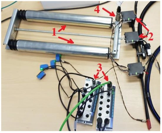
Figure 1.
Test bench for the experiment.
In Figure 1, two brushless DC motors (number 1 on the Figure) can be seen, with their drivers (number 2 on the Figure) and two I/O PROFINET modules (number 3 on the figure). For this experiment, only one motor was used, with a state of the art vibration sensor (number 4 on the picture) connected to it. The main parameters of the vibration sensor are given in Table 1, and of the motor in Table 2. For the rest of the equipment, product references are given in [15]. The I/O modules were used to send the vibration signals to the monitoring device—S7 Programmable locgic controller (PLC hereinafter) by PROFINET, which in turn sends the recorded vibration signal to the SIEMENS “Mindsphere” cloud for further processing. The parameters for the monitoring device used in the experiment are given in Table 3. From the cloud, the user can extract the data in the form of a CSV file with acceleration and time data. In Figure 2, the data acquisition devices of the experiment are displayed.

Table 1.
Technical parameters of the vibration sensor.
Table 2.
Technical parameters of the motor, used in the experiment.
Table 3.
Technical parameters of the monitoring device.
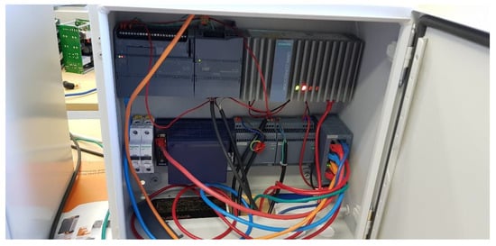
Figure 2.
Data acquisition devices.
This electrical box contains the SIMATIC S7 PLC used in this experiment (top left) and the “Mindsphere” gateway (top right). The vibration sensor can measure acceleration in 3 axes. It communicates directly with the PLC which is connected to the local Ethernet, the same as the gateway. The gateway then acquires data and sends it to the cloud, where user-friendly apps can display the interactive data and also detect anomalies, although only using a threshold. This accurate monitoring system can pick up 1 million samples of vibration data in just 10 seconds. The manufacturers reference for the vibration sensor, motor, I/O module, data gathering device and Mindsphere gateway are given in [18,19,20,21,22] respectively. The experiment was done in 3 cases to classify: a healthy motor, arcing stator (the motor requires maintenance but does not have to be stopped immediately), and an open circuit in one of the stator windings. So, 3 different signals, equal in length were monitored. A brushless DC motor is usually driven by a so-called three-phase DC signal. This is a pulse wide modulation signal (PWM) which is switched to the windings, which in turn acts in a similar way to a three-phase motor. This signal is displayed in Figure 3. One open circuit in the winding means that the motor cannot start, but if it is spinning and the fault happens, it still works with lots of vibrations and torque ripples. After some time, the motor stops and needs new windings.
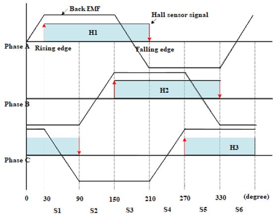
Figure 3.
Control signal and back EMF (electromotive force) of brushless direct-current (BLDC) motor.
From Figure 3 it can be seen that the signal is shifted 120 degrees between phases. Though it shares some similarities with the 3 phase permanent magnet synchronous motor, it is quite different, especially when monitoring vibrations. In the healthy motor FFT spectrum, the usual peaks, especially at 50 Hz, is missing in BLDC vibrations. The FFT of a healthy motor (1) and defective motor (2) are given in Figure 4. So, to conclude, deep networks here could achieve more accurate results, because in FFT analysis, only the amplitudes are higher for all three fault classes, which could be used for identification of fault existence itself, but not the identification of fault type. The form of the FFT is almost identical for healthy and for motors with an open circuit in the stator winding. This could be because FFT only applications are on stationary conditions. Fourier transform of the signal is obfuscation rather than a recovery of the information under dynamic conditions like in [17], where authors applied a recurrent neural network to detect BLDC motor bearing faults under non-stationary conditions (variable speed and torque). For this training, the information needed will be extracted from the static sequence of parameters, except for one class, arcing stator winding, which is hard to forecast and is unpredictable, but the speed or torque of the motor will be static. The neural network will be used to classify signals by the signal itself varying in the time domain. For the model to be fully applied for dynamic conditions though, it should be trained with variable-speed or torque.
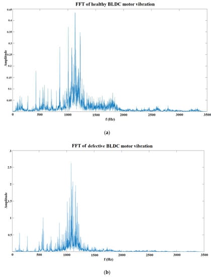
Figure 4.
Fast Fourier transform (FFT) of the vibrations of healthy (a) and defective (b) BLDC motors.
As can be seen from the first graph in Figure 4, most of the vibration peaks are at 1000–1200 Hz range. As previously mentioned, most of the peaks are the same, just with higher amplitude in the broken FFT.
2.2. Data Acquisition
The raw data acquired in the experiment described above is given in Figure 5.
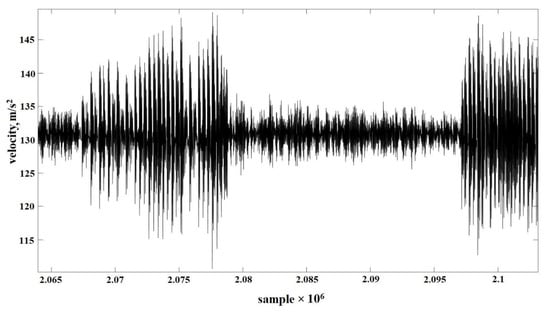
Figure 5.
Measured vibration signal.
Measurement was done for a total of 10 seconds for each of the motor conditions. The total training data contains 69 measurement samples with almost 50,000 points each, totaling more than 3 million points across all measurement samples. As can be seen from Figure 5, three characteristics of vibrations can be distinguished. The first part consisting of arcing winding, thus variable vibration amplitude can be seen in the graph. The middle part consists of normal vibrations with healthy motor characteristics and the last part consists of an open circuit in one winding. This is only one measurement with 50,000 samples where after an arc occurred, the motor lost one of the three phases.
2.3. Training Model
The typical architecture of an LSTM network is given in Figure 6. An LSTM is a deep network and a type of recurrent neural network (RNN), that is capable of learning long-term dependencies. They are widely used for signal, speech, and sound analysis and classification.
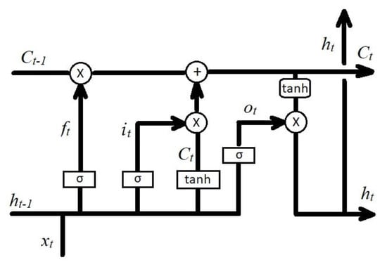
Figure 6.
Architecture of long short-term memory networks (LSTM) network nodes [12].
The training model will be done according to the nodes in Figure 6. There, yellow boxes represent hidden layers, pink ones are operational nodes, and arrows are vector transfers. The training model equations were used from [23,24]. In Neural Computation the first step, the information goes through the forget gate layer, where xt and ht−1 are either kept or deleted by a sigmoid layer, this is done with Equation (1).
where
- ft—decision to keep or discard data (equals to either 1 or 0),
- —information from previous nodes,
- —hidden layer,
- —weight matrices and bias vector parameters for learning,
- —weight matrices and bias vector parameters for learning.
In the second part of the training, it will be decided what information to store in the cell state. It is a two-part equation, where the sigmoid layer decides which values will be updated and then a new vector of values is created by a tanh layer. Then these two layers are combined to create an update. The combination is done in the X operational node in Figure 6. The calculations for this process are presented in Equations (2) and (3).
where
- —values that will be updated,
- —vector of new candidate values,
- —weight matrices and bias vector parameters for learning,
- —weight matrices and bias vector parameters for learning,
- —weight matrices and bias vector parameters for learning,
- —weight matrices and bias vector parameters for learning.
Then, the old cell state from the last LSTM layer Ct−1 is updated to a new cell state C. The update itself is described in the formulas above. The old state is multiplied by ft, and the other information is deleted (forgot), which was also decided in the first layers of the network, that is why this network is called short-term memory. Then the new candidate values are added and scaled by the amount, and decided to update each state value. This is described in Equation (4).
where
- —new cell state,
- —new, scaled candidate values,
- —old cell state,
- —decision whether to keep or discard data from the previous layer.
The last process of the training is where the output is decided. This process is divided into two parts with two equations. Firstly, which parts of the cell state are going to be outputted is decided by a sigmoid layer. Then the cell state goes through the tanh to push the values through −1 and 1 and is multiplied by the output of the sigmoid gate, so only parts that are relevant are outputted. This process is displayed in Equations (5) and (6).
where,
- —decided outputs,
- —weight matrices and bias vector parameters for learning,
- —weight matrices and bias vector parameters for learning,
- —the output to the next layer.
2.4. Feature Extraction
Now when the training process itself is described, the feature extraction from raw data for increasing model performance will be used. It was decided to use spectrograms of the signals for the feature extraction, for their great accuracy. The spectrogram is a visual representation of a signals frequencies spectrum as it varies in time. The spectrogram is generated using the Fourier transform.
The data chunks are Fourier transformed to calculate the magnitude of the frequency of each part. Each part corresponds to a vertical line in the image, this is a measurement of magnitude versus frequency for the specific time. These spectrums are then laid side by side to form an image. This process corresponds to the computation of the squared magnitude of the short-time Fourier transform of the signal. This is described in Equation (7).
where,
- t—time,
- —window width,
- STFT—short-time Fourier transform.
After the spectrograms are generated, the features from them are going to be extracted in two ways: spectral entropy and instantaneous frequency. Spectral entropy measures how spiky flat the spectrum of a signal is. Low spectral entropy means that a signal has a spiky spectrum (like a sum of sinusoids). A signal with a flat spectrum has high spectral entropy. The spectral entropy was calculated using Equations (8) and (9) from [25].
where,
- —the energy of frequency component,
- —is the probability mass function of the spectrum.
The Equation (8) is used for sub-band normalization before doing the entropy computation as suggested in [25]. After sub-band normalization, the spectral entropy was calculated using Equation (9).
Then, the instantaneous frequency will be applied to the same spectrograms. This function estimates the time-dependent frequency of a signal as the first moment of the power spectrum. This function is quite similar to previous computes spectrograms using short-time Fourier transforms over time windows. The function time outputs correspond to the centers of time windows. This function is calculated using Equation (10) from [26].
where,
- —instantaneous frequency,
- arg—complex argument function,
- —complex-valued function.
2.5. Feature Standardization
After eature extraction in two ways, it may mean that the data might differ too much and increase model bias. In order to use both of these features in one training model, their means have to be similar. When a network is fit on a large mean and large range of values, these large inputs could slow down network convergence and the model could lose effectiveness. After the extraction, their means will be calculated and checked if standardization is needed. The standardization or z-scoring will be done by the mean and standard deviation. Standardization will be done using Equations (11) and (12) from [27].
where,
- —standard deviation,
- —expected value (mean of the variable).
3. Results
3.1. Training with Raw Data
At first, the model was trained with raw data to get an idea of the complexity of the model needed. Additionally, it could be possible that raw data are easily interpreted and the model may achieve high accuracy.
For this training, an LSTM neural network model was constructed using a 5 × 1 layer array, which included:
- One sequence input layer—this is an input layer with one input dimension (amplitude of the vibration);
- BiLSTM—bidirectional long short-term memory layer described in Section 2.3. The layer was designed with 200 hidden units (neurons) in the layer. This command instructs the layer to map the input time series into 200 features and prepares the output to the fully connected layer;
- Three fully connected layers—this layer instructs the model to specify the output into three classes;
- Softmax layer—where the exponential of the input vector is computed in order to normalize the data set into a probabilistic distribution with values that sum to one.
- A classification layer.
For this training, the ADAM—adaptive moment estimation solver was used. ADAM is better with LSTMs than a standard stochastic gradient descent with momentum solver.
For this training, 150 epochs were used to extend the training, since it is expected to take some time, because of the big proportions of data.
The initial learning rate of 0.02 was selected with a piecewise training function to drop the learning rate by a factor of 0.1, decreasing the learning rate to 0.002 after 30 epochs. The learning rate is one of the most important factors to consider because a learning rate that is too high means that the model may train too rapidly, jumping between low and high errors. A learning rate that is too low could mean that the model may take too long to increase performance and reach the max epochs before achieving good training. This parameter is usually guessed from experience and modified by trial and error.
The gradient threshold was set to 1, to stabilize the training process by preventing the gradients from getting too large.
Lastly, after doing some test runs on the training, it ran out of graphics card memory, so to prevent that, the data was split into the minibatch size of 5. Meaning one train epoch will take 12 iterations each.
The training process is given in Figure 7 and the results are represented in the form of a confusion matrix in Figure 8. The confusion matrix is obtained after the training process itself and is a very good classification result summary. Mainly the trained model is used again to test the classification against real data. If the model classifies the output the same as the target, then it appoints the result to the green diagonal cubes of the matrix, thus counting as correct classification. If the model classifies incorrectly, then it goes to red cubes, according to incorrect classes that they were classified, meaning that the total accuracy equals to the sum of all true positives and true negatives (correct classifications), subtracted by the sum of true positives, true negatives, false positives, and false negatives. The training process was done using Equations (1)–(6).
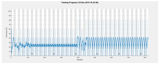
Figure 7.
Training process with raw data.
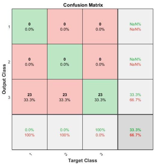
Figure 8.
Training results with raw data in the form of a confusion matrix.
As can be seen from the results, the training performed with a very high error. It averaged around 20–30 percent accuracy, until the learning rate drop at 30 epochs. The drop rate only slightly increased the accuracy to around 30%. However, it also induced rapid changes in the training process as mentioned above. The learning rate drop made the training accuracy jump from 18 to 42% accuracy from iteration to iteration.
The training results are summarized in the form of a confusion matrix in Figure 8. There, the target and output results are shown. As can be seen, the model misinterpreted the data and classified all of it as class 3—open contact in one of the windings. This can happen because of the immense size of the raw data set and also because of the complexity of the data itself. The change of parameters did not submit more accurate results than the training mentioned above.
Because of the low performance of the training, a method to decrease complexity and extract the features from the data will be used in the next chapter.
3.2. Training with Feature Extraction and Standardization
After achieving mediocre results with raw data, it was decided to try and improve training performance with feature extraction, a useful and widely used data processing tool for machine learning applications. The raw data given in Figure 9 was first converted into spectrograms using Equation (7). The resulting spectrograms of each of the classes for one 50,000 sample signal each are presented in Figure 10.
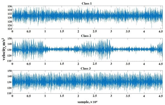
Figure 9.
Raw signal with 50,000 samples for each of the classes.
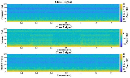
Figure 10.
Spectrograms of each of the signal classes.
From Figure 10, there is no great difference between classes, compared with raw signals in Figure 9. However after features are extracted, the difference can be seen. Spectral entropy was applied to the training dataset using Equations (8) and (9), also the instantaneous frequency calculations were applied to the whole dataset using Equation (10) and the results of both calculations of the signals for each of the classes are given in Figure 11.
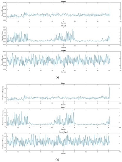
Figure 11.
Three signals with features extracted, using spectral entropy (a) and instantaneous frequency (b).
For the new training, two datasets are prepared, one with instantaneous frequency and the other with spectral entropy applied. With the two datasets combined, a signal with two amplitudes can be created instead of one, adding an extra feature to the training. Now the dataset contains two one-dimensional signals. This can significantly improve the training.
After the feature extraction, the data must be standardized. This means that both of the signals’ amplitudes must be on the same order of magnitude. Both of the signals means are calculated and the results are given below:
- Mean of instantaneous frequency signal—1.0684
- Mean of spectral entropy signal—0.3644
It is clear that the signals must be standardized. For standardization, the mean and standard deviation will be used to standardize all of the signals in the training dataset. This was done using calculations from Equations (11) and (12). The results are given below:
- Mean of instantaneous frequency signal—−0.6006
- Mean of spectral entropy signal—−0.6089
Now, since the signals are on the same order of magnitude, the training itself can be repeated, using the same parameters as previously. The only thing that must be changed in the model itself is another sequence input layer added, totaling a number of two layers. This is because now the dataset consists of two signals.
Additionally, after a few test runs, it was decided to lower the number of hidden units in the BiLSTM layer to a total of 120, since the training data after the feature extraction consist of 69 samples (23 for each of the classes), each with two one-dimensional signals consisting of 255 sample points instead of 50,000 each. This should also significantly increase the speed of the training process, which in turn allows us to increase the minibatch size. The training process is given in Figure 12.
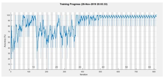
Figure 12.
Training process with standardized data.
From Figure 12 it can be seen that the training reached maximum performance at 40 epochs. For this training, a learning rate of 0.01 was used, with a piecewise training algorithm that drops the learning rate by a factor of 0.1 after 30 epochs. Because of that, after 30 epochs, the actual learning rate was 0.001. It learned much faster and more accurately because of the successful feature extraction and standardization, also it required significantly fewer computer resources, even allowing us to perform the training on the computer’s central processor instead of the graphics unit. The training reached a performance of 97.10%. The results in the form of a confusion matrix are given in Figure 13.
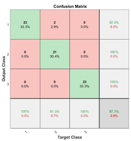
Figure 13.
Confusion matrix of training with 97.10% accuracy.
From Figure 13, an assumption can be made that the model accurately classified the data into correct classes, except for two samples, that were classified incorrectly as class 1 instead of class 2. That may happen if there were no arcs in the stator and it worked correctly, thus confusing the model. That may happen when the data set is quite small. In this case, 23 signals for each of the classes is not that much, but nonetheless, the training achieved quite high accuracy, which can be advanced to further research.
4. Conclusions and Discussions
A vibration dataset containing three classes of normal, arcing, and open circuit in BLDC motors stator was gathered using vibration sensors, data gathering devices and cloud technologies.
A one dimensional dataset consisting of 69 signal measurements, 23 for each class with 50,000 sample points of amplitude, totaling more than 3 million sample points were prepared for training.
In response to poor training with raw data, to increase the training performance, feature extraction and standardization were applied to the dataset. This included producing spectrograms for all signals in the dataset and extracting the features, using instantaneous frequency and spectral entropy. The two one-dimensional signals produced were then consolidated to one signal as two-dimensional data, in order to produce 69 datasets with two feature signals for each, thus increasing training performance. To prepare the data for training after feature extraction, the datasets were standardized using mean and standard deviation, to level the magnitudes of the signals, avoiding model confusion during training. The number of hidden units in the BiLSTM layer was reduced to 120 and another sequence input layer added, adding up to two layers in total, to use both signals as two-dimensional data. The learning rate was reduced to 0.01 with a piecewise training algorithm to drop the learning rate by a factor of 0.1 to a total of 0.001 after 30 epochs. The training achieved a 97.10 training error, with two samples of data incorrectly classified.
Although two sets of data were classified incorrectly, which could happen if the motor was working correctly at the time. That means if sparking happens, the model would still classify it correctly. The model, however, stillachieved very high performance and an assumption can be made that it would correctly classify BLDC motor stator status. This research can be further enhanced by applying the trained model for the real experiment and testing it in a real environment.
Additionally, the sampling rate and sensitivity of the vibration sensor allowed us to achieve very detailed vibration graphs. This high-performance technology could ease the process of fault detection and classification, allowing the detection of all possible faults and anomalies at both static and dynamic conditions by using only one measurement. As high detailed data must be preprocessed before modeling because of the size of data sets, not only the training process becomes very slow, but it is hard to work with that much data. Feature extraction helps to reduce the size of datasets, not only increasing performance and training speed but also allowing to train the deep network on CPU.
Because there are not many publications regarding this topic, it should generate a lot of interest in BLDC analysis, since this type of motor is widely used. It is also quite different from traditional induction machines, which indicates a need for more research and also different diagnostic approaches. Predicting stator faults is a very important topic because it is one of the most occurring defects. It could happen instantly, where prediction is not necessarily needed, or it can occur slowly by firstly only arcing, where correct prediction could mean saved resources by cheaper repairs and guarantee of a nonstop production process.
Unfortunately, because of the lack of resources for practical experiments for this research, it was not possible to apply the working model to the experiment and an assumption had to be made that model can classify the data in theory correctly. Further enhancements can be made by combining this vibration analysis model with other fault detection using vibration analysis techniques. For example, bearing condition monitoring and fault detection, or other faults described in the introduction of this research. The combination of these fault diagnostic models could lead to a self-diagnosing motor by using only vibration analysis. The authors are pursuing this research and are planning to design this combined model and publish another article in the near future.
Author Contributions
All authors contributed to this paper: conceptualization, T.Z. and J.V.; methodology, J.V. and T.Z.; validation, T.Z., J.V. and A.K.; data curation, K.D.; model architecture and training, T.Z.; writing—original draft preparation, K.D. and A.K.; writing—review and editing, K.D. and A.K.; visualization, T.Z.; supervision, M.A. All authors have read and agreed to the published version of the manuscript.
Funding
This research received no external funding.
Conflicts of Interest
The authors declare no conflict of interest.
References
- Chaudhari, Y.K.; Gaikwad, J.A.; Kulkarni, J.V. Vibration Analysis for Bearing Fault Detection in Electrical Motors. In Proceedings of the 2014 First International Conference on Networks & Soft Computing (ICNSC2014), Guntur, India, 19–20 August 2014. [Google Scholar]
- Tsypkin, M. Induction Motor Condition Monitoring: Vibration Analysis Technique—A Practical Implementation. In Proceedings of the 2011 IEEE International Electric Machines & Drives Conference (IEMDC), Niagara Falls, ON, Canada, 15–18 May 2011. [Google Scholar]
- Zhang, S.; Qu, Y.; Han, Q.; Yong, Y. Vibration Fault analysis for rotor systems by using Hilbert spectrum. In Proceedings of the 2010 International Conference on Mechanic Automation and Control Engineering, Wuhan, China, 3 August 2010. [Google Scholar]
- Ko, H.S.; Kim, K.J. Characterization of Noise and Vibration Sources in Interior Permanent-Magnet Brushless DC Motors. IEEE Trans. Magn. 2004, 40, 3482–3489. [Google Scholar] [CrossRef]
- Yoon, T. Magnetically Induced Vibration in a Permanent-Magnet Brushless DC Motor With Symmetric Pole-Slot Configuration. IEEE Trans. Magn. 2005, 41, 2173–2179. [Google Scholar] [CrossRef]
- Rajagopalan, S.; Habetler, T.G.; Harley, R.G.; Sebastian, T.; Lequesne, B. Current/Voltage-Based Detection of Faults in Gears Coupled to Electric Motors. IEEE Trans. Ind. Appl. 2006, 42, 1412–1420. [Google Scholar] [CrossRef]
- Pramesti, W.; Damayanti, I. Stator fault identification analysis in induction motor using multinomial logistic regression. In Proceedings of the 2016 International Seminar on Intelligent Technology and Its Applications (ISITIA), Lombok, Indonesia, 23 January 2017. [Google Scholar]
- Pietrowski, W.; Górny, K. Wavelet torque analysis and neural network in detection of induction motor inter-turn short-circuit. In Proceedings of the 2017 18th International Symposium on Electromagnetic Fields in Mechatronics, Electrical and Electronic Engineering (ISEF) Book of Abstracts, Lodz, Poland, 2 November 2017. [Google Scholar]
- Zarei, J.; Poshtan, J.; Poshtan, M. Bearing fault detection in induction motor using pattern recognition techniques. In Proceedings of the 2008 IEEE 2nd International Power and Energy Conference, Johor Bahru, Malaysia, 27 January 2009. [Google Scholar]
- Wallsheid, O.; Kirchgassner, W.; Bocker, J. Investigation of Long Short-Term Memory Networks to Temperature Prediction for Permanent Magnet Synchronous Motors. In Proceedings of the 2017 International Joint Conference on Neural Networks (IJCNN), Anchorage, AK, USA, 14–19 May 2017. [Google Scholar]
- Luo, Y.; Qiu, J.; Shi, C. Fault Detection of Permanent Magnet Synchronous Motor Based on Deep Learning Method. In Proceedings of the 2018 21st International Conference on Electrical Machines and Systems (ICEMS), Jeju, Korea, 7–10 October 2018. [Google Scholar]
- Khan, T.; Alekhya, P.; Seshadrinath, J. Incipient Inter-turn Fault Diagnosis in Induction motors using CNN and LSTM based Methods. In Proceedings of the 2018 IEEE Industry Applications Society Annual Meeting (IAS), Portland, OR, USA, 23–27 September 2018. [Google Scholar]
- Xiao, D.; Huang, Y.; Zhang, X.; Shi, H.; Liu, C.; Li, Y. Fault Diagnosis of Asynchronous Motors Based on LSTM Neural Network. In Proceedings of the 2018 Prognostics and System Health Management Conference, Chongqing, China, 26–28 October 2018. [Google Scholar]
- Lee, K.; Kim, J.; Kim, J.; Hur, K.; Electrical, H.; Engineering, E. Stacked Convolutional Bidirectional LSTM Recurrent Neural Network for Bearing Anomaly Detection in Rotating Machinery Diagnostics. In Proceedings of the 2018 1st IEEE International Conference on Knowledge Innovation and Invention, Jeju, Korea, 23–27 July 2018. [Google Scholar]
- Kumar, T.C.A.; Singh, G.; Naikan, V.N.A. Sensitivity of Rotor Slot Harmonics due to InterTurn Fault in Induction Motors through Vibration Analysis. In Proceedings of the 2018 International Conference on Power, Instrumentation, Control and Computing (PICC), Thrissur, India, 18–20 January 2018. [Google Scholar]
- Musthofa, A.; Asfani, D.A.; Negara, I.M.Y.; Fahmi, D.; Priatama, N. Vibration Analysis for the Classification of Damage Motor PT Petrokimia Gresik Using Fast Fourier Transform and Neural Network. In Proceedings of the 2016 International Seminar on Intelligent Technology and Its Applications (ISITIA), Lombok, Indonesia, 28–30 July 2016. [Google Scholar]
- Abed, W.; Sharma, S.; Sutton, R.; Motwani, A. A Robust Bearing Fault Detection and Diagnosis Technique for Brushless DC Motors Under Non-stationary Operating Conditions. J. Control Autom. Electr. Syst. 2015, 26, 241–254. [Google Scholar] [CrossRef]
- Vibration Sensor Reference. Available online: https://support.industry.siemens.com/cs/products/6at8002-4ab00/siplus-cms2000-vib-sensor-s01?pid=246139&mlfb=6AT8002-4AB00&mfn=ps&lc=en-GB (accessed on 6 February 2020).
- Motor Reference. Available online: https://www.rulmeca.com/en/products_unit/catalogue/2/industrial_unit_handling/12/drive_rollers_and_components_for_unit_handling_industrial_applications (accessed on 6 February 2020).
- I/O Module Reference. Available online: https://new.siemens.com/global/en/products/automation/systems/industrial/io-systems/simatic-et-200eco-pn.html (accessed on 6 February 2020).
- PLC for Monitoring Reference. Available online: https://new.siemens.com/global/en/products/automation/products-for-specific-requirements/siplus-cms.html (accessed on 6 February 2020).
- Mindsphere Gateway. Available online: https://support.industry.siemens.com/cs/pd/695057?pdti=td&dl=en&lc=en-NL (accessed on 6 February 2020).
- Hochreiter, S.; Schmidhuber, J. Long short-term memory. Neural Comput. 1997, 9, 1735–1780. [Google Scholar] [CrossRef] [PubMed]
- Gers, F.A.; Schmidhuber, J.; Cummins, F. Learning to Forget: Continual Prediction with LSTM. Neural Comput. 2000, 12, 2451–2471. [Google Scholar] [CrossRef] [PubMed]
- Toh, A.; Togneri, R.; Nordholm, S. Spectral entropy as speech features for speech recognition. Proc. PEECS 2005, 1, 92. [Google Scholar]
- Blackledge, J.M. Digital Signal Processing: Mathematical and Computational Methods, Software Development and Applications, 2nd ed.; Woodhead Publishing: Cambridge, UK, 2006; p. 134. ISBN 1904275265. [Google Scholar]
- Kreyszig, E. Advanced Engineering Mathematics, 4th ed.; Wiley: Hoboken, NJ, USA, 1979; p. 880. ISBN 0-471-02140-7. [Google Scholar]
© 2020 by the authors. Licensee MDPI, Basel, Switzerland. This article is an open access article distributed under the terms and conditions of the Creative Commons Attribution (CC BY) license (http://creativecommons.org/licenses/by/4.0/).