Experimental Investigation on Time-Frequency Characteristics of Microseismic Signals in the Damage Evolution Process of Coal and Rock

Abstract

The deformation and failure of coal and rock materials is the primary cause of many engineering disasters. How to accurately and effectively monitor and forecast the damage evolution process of coal and rock mass, and form a set of prediction methods and prediction indicators is an urgent engineering problems to be solved in the field of rock mechanics and engineering. As a form of energy dissipation in the deformation process of coal and rock, microseismic (MS) can indirectly reflect the damage of coal and rock. In order to analyze the relationship between the damage degree of coal and rock and time-frequency characteristics of MS, the deformation and fracture process of coal and rock materials under different loading modes was tested. The time-frequency characteristics and generation mechanism of MS were analyzed under different loading stages. Meanwhile, the influences of properties of coal and rock materials on MS signals were studied. Results show that there is an evident mode cutoff point between high-frequency and low-frequency MS signals. The properties of coal and rock, such as the development degree of the original fracture, particle size and dense degree have a decisive influence on the amplitude, frequency, energy and other characteristic parameters of MS signals. The change of MS parameters is closely related to material damage, but has no strong relation with the loading rate. The richness of MS signals before the main fracture depends on the homogeneity of materials. With the increase of damage, the energy release rate increases, which can lead to the widening of MS signals spectrum. The stiffness and natural frequency of specimens decreases correspondingly. Meanwhile, the main reason that the dominant frequency of MS detected by sensors installed on the surface of coal and rock materials is mainly low-frequency is friction loss and the resonance effect. In addition, the spectrum and energy evolution of MS can be used as a characterization method of the damage degree of coal and rock materials. Furthermore, the results can provide important reference for prediction and early warning of some rock engineering disasters.

1. Introduction

Although many countries and regions in the world have reduced the use of coal, some countries, e.g., China, India and South Africa, remain heavily dependent on coal resources. Coal consumption still accounts for a large proportion in the energy consumption structure in these countries. With the depletion of shallow coal resources, especially in China, mining depth of a coal mine increases sharply, and high ground stress, high ground temperature, hyperosmosis and strong disturbance problems are gradually emerging. In the complex environment, coal and rock materials are under long-term high loading condition, and internal damage degree is more serious compared to shallow mining. The normal mining disturbance is also easy to induce the deformation and fracture of coal or rock materials and then cause serious hazards, such as rock burst, coal and gas outburst and large deformation of surrounding rock [1,2]. Influenced by environmental protection and policy orientation, the proportion of oil, natural gas and new energy in the disposable energy structure has increased. The study on the damage of coal and rock in the development of these resources should also be getting enough concern. The reason is that in the process of shale gas or natural gas exploitation and gas extraction, hydraulic fracturing is often used to cause deformation and failure of coal and rock mass, so as to increase the permeability of coal and rock mass to achieve high production. Thus, the damage degree of coal and rock mass directly affects the production of oil and gas wells. Meanwhile, with the expanding excavation of underground cavern and tunnel of hydropower station, underground storage cavern and slope, the problem about deformation and failure of surrounding rock are also becoming increasingly apparent, which has a serious impact on the construction and operation of the project. Thus, how to accurately and effectively monitor and forecast the damage evolution process of coal and rock mass, and form a set of prediction methods and indicators is an urgent engineering problem to be solved.

As a form of energy dissipation in the process of coal and rock damage, MS accompany the whole process of deformation and fracture of coal and rock and can reflect the internal damage evolution process of coal and rock in real time. MS monitoring technology has been widely applied to source location [3,4], safety design [5], prediction and early warning of disasters [6,7], etc. in mine, tunnel cavern, diversion tunnel of hydropower station, underground storage cavern, slope excavation, etc. For example, Zhu et al. [8], Ding et al. [9] and Wang et al. [10] conducted experimental investigation on the MS frequency response before the coal and rock dynamic disasters, such as coal and gas outburst, mine rock and rock burst, and found that the frequency spectrum distribution of MS varied in the damage evolution process of coal and rock and frequency spectrum law can reflect the damage degree of coal or rock to some extent. He et al. [11] used the MS frequency index and energy index to monitor mining disturbance and geological anomaly of the coal seam and this method could realize reliable detection of distribution characteristics of static load stress field in coal seam area. Zhu et al. [12] adopted arrival times of the MS P-phase to collect the MS signal of hydraulic fracturing of the coal seam, and then realize the fracture tracking and effect evaluation. Maity and Ciezobka [13] discussed how b-value distribution provides insights into the rock type as well as the interaction with pad scale faults in shale reservoirs, and believed the in-situ stress state had a significant bearing on the b-value and there was a significant impact of in-situ discontinuities and rock brittleness on the microseismicity distributions. The analysis of the microseismic b-value provides a template for future applications where MS surveys are available. Chen et al. [14] introduced an improved matching and locating technique to detect and locate MS events (4 < ML < 0) associated with the hydraulic fracturing treatment and adopted clustering behavior including b- and D-value distributions to understand shale stimulation behavior, and firstly demonstrated the detectability and location accuracy of the proposed approach with a pseudo-synthetic data set. Martínez-Garzón et al. [15] applied state of the art seismological processing schemes to the continuous seismic waveform recordings and confirmed that MS monitoring of reservoir treatment could contribute towards improved reservoir monitoring and leakage detection. Mao et al. [16], Ma et al. [17] and Dai et al. [18] used the MS monitoring technology to monitor and analyze the microfracture evolution in the surrounding rock of the cave in real time. The relationship between temporal and spatial evolution of MS and the rock burst was revealed. The results showed that MS activities generally have time priority and spatial consistency to rock burst events, which could provide a basis for rock burst prediction of tunnel and microseismic monitoring and early warnings. Xu et al. [19] quantitatively evaluated the relationship between microseismic activities induced by rock mass damage during slope instability, strength degradation and dynamic instability of the slope are explored, and the slope stability. Then, they proposed a dynamic evaluation method of rock slope stability considering the effects of MS damage. They argued that MS activity induced by construction disturbance only slightly affects the stability of the slope. The proposed feedback analysis technique provided a method for dynamically assessing rock slope stability and could be used to assess the slope stability of other similar rock slopes. Through the above analysis, we can know that MS monitoring technology can be applied in many aspects. The main reason lies in the close relationship between the MS signal and deformation and failure of coal and rock materials. MS signals can indirectly reflect the damage of coal and rock materials, so as to realize disaster prediction or the effect evaluation of hydraulic fracturing.

In previous studies, it was confirmed that the MS parameters, such as amplitude, event number and frequency, which could reflect the quantity, size and direction of microcrack propagation, had a great relevance on damage degree of coal and rock [20,21,22,23]. The actual MS signals contain a great amount of noise whose interference often results in the difficulty of the signal processing. Therefore, accurate identification of MS is of important theoretical significance to coal damage criterion.

MS identification can be reflected directly or indirectly by the following two methods: characteristic parameter analysis and wave spectrum analysis. The former reveals MS monitoring mechanism of the source and precursors law of rock mass failure by means of statistical analysis of MS events number, event count, amplitude, b value and energy count. Especially, the distribution of event count, amplitude and energy count is consistent with energy distribution. Many researches have been devoted to the application of characteristic parameter analysis method in rock engineering. For instance, Blake et al. [24] and Lu et al. [25] found that there were obvious anomaly MS events counts before rock burst by monitoring MS events induced by hard rock fracture. Ma et al. [26] and Xia et al. [27] quantitatively studied advance support pressure distribution rule of working face by analyzing corresponding relation between MS events number and support stress. He et al. [28] evaluated dynamic and static stress disturbance through seismic wave velocity to predict the rock burst risk. Wu et al. [29] believed that the sudden release of accumulated strain energy in rock mass had a performance of abrupt change of cumulative number of MS events, which can be used as rock instability and failure precursor. Kwiatek et al. [30] analyzed the b value variations over successive seismic cycles in laboratory stick-slip experiments. Chen et al. [31] insisted that weak MS activity meant energy accumulation for strong shock, which can be used to forecast the danger of a rock burst.

Recently, there is more and more interest in the wave spectrum analysis method to acquire MS characteristics. The frequency spectrum of the MS signal is rich, and its main frequency varies from a few Hertz to several hundred Hertz. Specific damage mechanisms generate specific MS spectrum. In previous studies, the mathematical analysis method was extensively applied in to analyze the distribution of the main frequency of MS signals. Ge [32] and Errington et al. [33] analyzed the energy spectral density characterization of MS events in two potash mines and found that peak frequency of MS signals is approximately 38 Hz or 54 Hz. Lu et al. [34] studied the spectrum characteristics of MS signals monitored in situ, such as coal and gas outburst, rock burst, pressure release blasting, etc., and found that before a coal and gas outburst occurred, the low-frequency component of 0–10 Hz changed significantly, and the relatively high-frequency component of 90–240 Hz increased correspondingly. However, the main frequency of the precursor signal of a rock burst was below 50 Hz, the main frequency of the coal seam pressure release blasting was below 20 Hz and the main frequency of the roof pressure relief blasting was between 10 and 150 Hz. Li et al. [35] compared and analyzed the propagation law of MS signals between coal layers under vertical bedding and parallel bedding, and concluded that MS signals had a small attenuation along the bedding, but a large amplitude attenuation and signal delay in the direction of vertical bedding. Meanwhile the frequency spectrum of MS signals was obtained using the Hilbert–Huang Transform (HHT), and the main frequency of MS signals was between 20 and 100 Hz. Yuan [36] obtained the spectrum characteristics and distribution change rule of MS using Fourier transform (FFT) and fractal geometry theory. However, for nonlinear and non-stationary signal, e.g., MS, it is hard to find the right time window to accommodate different time periods of signal using FFT or short time Fourier transform. Therefore, it can not achieve a good effect to employ FFT or short time Fourier transform to analyze the instantaneous characteristic of MS signals. Capilla C [37] and Zhu et al. [38] employed a wavelet and wavelet packet analysis to research the MS spectrum characteristics. However, the denoising effect of wavelet transform depends much on the selection of wavelet function, decomposition scale and threshold value. As a time-frequency analytical method, HHT was more adaptive and superior to FFT or wavelet [39]. Li et al. [35] and Wang et al. [40] investigated the propagation law of MS signals under different loading direction and obtained Hilbert spectrum by using HHT.

In previous studies, the variation law of time-frequency parameters in the process of deformation and failure of coal and rock materials from the perspective of phenomena received more attention. However, there are few investigations on the relationship model between MS and damage of coal and rock materials. Meanwhile, the intrinsic mechanism of the frequency variation of MS signals under different damages is rarely explained. Moreover, due to a different loading mode and loading stage, the corresponding damage degree of coal and rock will be different, and the time-frequency characteristics of the MS signals will also change dynamically. In addition, due to the different components and structures of coal and rock, the corresponding deformation and fracture processes of coal and rock will be greatly different, which will also lead to great differences in the variation characteristics of MS signals. However, the influence of loading mode, loading stage, particle size, strength and weak surface of structure of coal and rock materials on time-frequency characteristics of MS signals received little attention in previous studies.

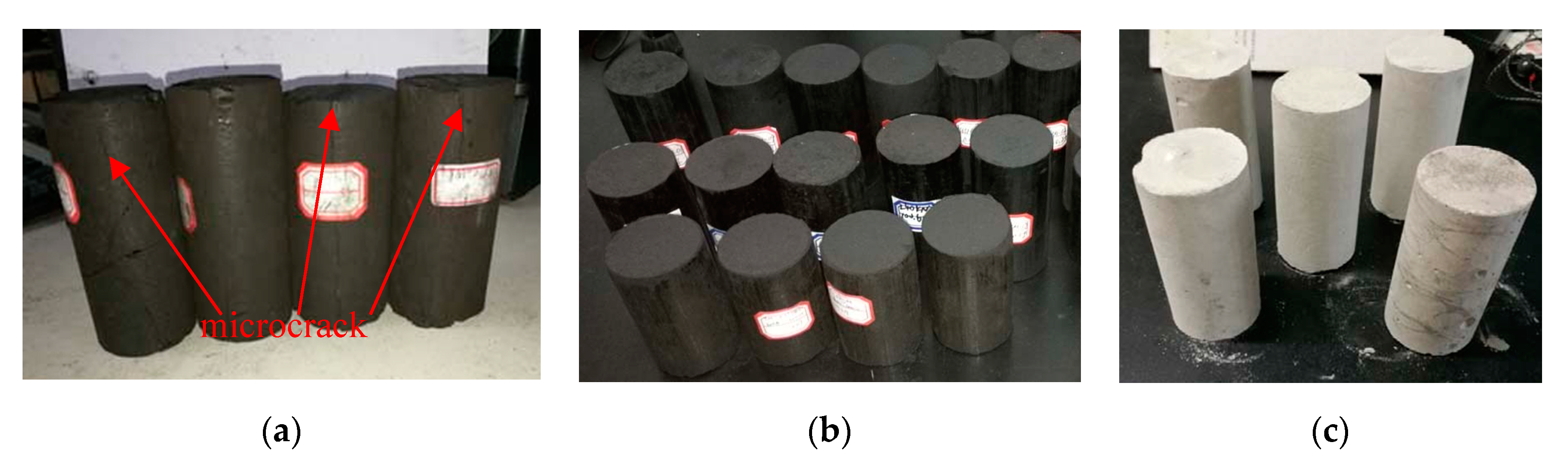
Realizing the limitations, the deformation and fracture experiment of raw coal, shaped coal and cement specimen under different load mode (constant speed, variable speed and graded loading) is set up in the paper and a de-noising analysis method based on the empirical mode decomposition (EMD) and wavelet threshold method is put forward. In addition, time-frequency characteristics of MS signals at different loading stages are researched and the intrinsic reason of the spectrum evolution law of MS signals of coal and rock materials is proposed theoretically. Finally, the influence of loading mode, loading stage, particle size, strength and weak surface of structure of coal and rock materials on MS signals is studied.

2. Experimental Description

2.1. Testing Specimens

2.1.1. Raw Coal Specimens

The raw coal specimens were taken from the Laohutai Coal Mine of the Fushun mining group corporation Ltd. in China. To avoid the mining influence, sampling sites were selected in the places, which were 100 m outside from the working face of the upper gate road of 55002#. Testing specimens belonged to hard coal and had clear bedding, as shown in Figure 1a. In order to keep the initial state of the coal sample as far as possible, dry drilling, dry cutting and dry grinding under low velocity were used in the process of specimen preparation. There were ten specimens, which met the suggested method of International Society for Rock Mechanics (ISRM) [41,42] after eliminating the coal sample whose surface had evident microcrack. The sizes of the six specimens were both with a diameter of 50 mm and height of 100 mm.

2.1.2. Shaped Coal Specimens

Shaped coal specimens were taken from the 24080 working face in 10th coal mine of Pingdingshan Tian’an Coal Industry CO., LTD in China. Two standards, i.e., the preparation method of the coal sample (GB 474-2008) [43] and standard test methods for physical and mechanical properties of concrete (GBT2050081-2019) [44] provided reference for the sampling, crushing, screening, preparation and curing of shaped coal specimens. The shape and size met the suggested method of ISRM [41,42]. The coal samples taken in the field were crushed by the pulverizer, and the crushing granularities are respectively 0.50–2.00 mm, 0.25–0.50 mm and less than 0.25 mm. Three kinds of pulverized coal particles were put into a molding tool under a molding pressure of 10 MPa. In the molding process, an appropriate amount of coal tar was added in the samples and the molds released after 24 h. Air curing was adopted for the specimens, and the specimens were naturally cured indoors. The curing temperature was maintained at 20 ± 2 °C, the humidity was above 95% and the curing time was 28 days. The three shaped coal specimens of three kinds of particles were made respectively and all specimens were with a diameter of 50 mm and height of 100 mm, as shown in Figure 1b.

2.1.3. Cement Specimens

The cement used in the experiment was P.O 42.5 ordinary Portland cement produced by Anhui Conch Cement Co., Ltd. in China. The preparation and curing of cement specimens were mainly based on standard test methods for physical and mechanical properties of concrete [44]. The shape and size met the suggested method of ISRM [41,42]. The water-cement ratio was 0.45 and the molding and curing process was similar to shaped coal specimens. The cement specimens were all with a diameter of 50 mm and height of 100 mm, as shown in Figure 1c.

2.2. Experimental System

The coal and rock damage experiment system under uniaxial compression employed a high-accuracy Servo material testing machine, which could control the loading rate and adjust oil-pressure. The system was mainly not only used to determine uniaxial compressive strength of coal, but also tested the variation law of MS. The system included YAW-1000 servo pressure testing machine, press data recording system, MS dynamic data acquisition system, etc. The structure diagram of system is shown in Figure 2.

Coal and rock fracture experiment under uniaxial compression was completed in a state key laboratory of coal resources and safe mining of China University of Mining and Technology, Beijing. The loading system adopted the YAW series microcomputer control electro-hydraulic servo pressure testing machine system, which can synchronously and automatically record the stress, longitudinal strain, lateral strain, etc. MS sensors employed the SF1500MEMS capacitive accelerometer produced by COLIBRYS Company. MS sensors had the following parameters: the linear acceleration range was ±3 g, corresponding sensitivity was 1.2 V/g and frequency response range was from 0 to 1500 Hz, especially the frequency response range was from 0 to 5000 Hz for the weak signal. Preamplifier gain was 40 db. The cRIO-9074 embedded machine control and monitoring system produced by National Instruments Corporation (NI) was used to acquire data. NI cRIO-9074 had a 400 MHz industrial real-time processor and two 10/100 Mb/s Ethernet ports. The A/D converter was 16 bits. The data sample rate was 2500 per second.

2.3. Experimental Loading Scheme

The loading for uniaxial compression tests on 1#-6# coal specimens were controlled by the axial load rate. In order to eliminate the influence of contingency factors, two MS sensors were arranged on coal surface in the experiment process (as shown in Figure 3). The experimental loading scheme is shown in

Table 1. Experimental scheme and damage of raw coal specimens.

Experiment Number	Sample Number	Loading Rate	Peak Force (Fmax) (KN)	Damage State
Y1	1#	30 N/s	32.580	ruptured
Y2	2#	50 N/s	18.099	ruptured
Y3	3#	40 N/s	111.918	ruptured
Y4	4#	Multi-stage loading: ① 10 N/s, 1000 s duration; ② Maintain 25 KN, 10 s duration; ③ 200 N/s until sample rupture.	55.342	ruptured
Y5	5#	Multi-stage loading: ① 50 N/s reaching to 7 KN, then maintain 30 s at 7 KN; ② 30 N/s reaching to 10 KN, then maintain 30 s at 10 KN; ③ 20 N/s reaching to 12 KN, then maintain 30 s at 12 KN; ④ 15 N/s to 15 KN, then maintain 30 s at 15 KN; ⑤ 10 N/s until sample rupture.	19.950	ruptured
Y6	6#	Multi-stage loading: ① 20 N/s reaching to 5 KN, then maintain 30 s at 5 KN; ② 6 N/s reaching to 6 KN, then maintain 30 s at 6 KN; ③ 3 N/s reaching to 7 KN, then maintain at 7 KN	7.014	non-ruptured

.

The loading procedure of shaped coal was the same as that of raw coal. Constant speed and “force-time” loading method was adopted. There were 4 loading speeds with 5 N/s, 10 N/s, 20 N/s and 30 N/s, respectively. Loading schemes and failure conditions of shaped coal specimens with different particle sizes are shown in

Table 2. Experimental scheme and damage of shaped coal specimens.

Experiment Number	Particle Size (mm)	Loading Rate (N/s)	Peak Force (Fmax) (KN)	Peak Stress (σc) (MPa)	Damage State
X1	Less than 0.25	10	7.738	0.77	ruptured
X2	Less than 0.25	20	12.002	1.20	ruptured
X3	Less than 0.25	30	20.252	2.02	ruptured
X4	0.25–0.50	5	2.738	0.27	ruptured
X5	0.25–0.50	10	2.322	0.23	ruptured
X6	0.25–0.50	20	10.724	1.07	ruptured
X7	0.50–2.00	5	2.416	0.24	ruptured
X8	0.50–2.00	10	3.176	0.27	ruptured
X9	0.50–2.00	20	31.536	3.15	ruptured

.

The loading procedure and failure conditions of cement specimens are shown in

Table 3. Experimental scheme and damage of cement experiment.

Experiment Number	Loading Rate (N/s)	Peak Force (Fmax) (KN)	Peak Stress (σc) (MPa)	Damage State
S1	200	162.959	16.30	ruptured
S2	150	123.217	12.32	ruptured
S3	250	196.591	19.66	ruptured
S4	150	166.175	16.62	ruptured
S5	200	229.457	22.95	ruptured
S6	250	248.486	24.84	ruptured
S7	150	118.913	11.89	ruptured
S8	150	126.291	12.63	ruptured

. Constant speed and “force-time” loading method was also adopted. There were 3 loading rates with 150 N/s, 200 N/s and 250 N/s, respectively.

2.4. MS Signal Parameters

According to the different description methods, the parameters of MS signals can be divided into state parameters and process parameters. The former mainly reflects the instantaneous behavior of MS signals, while the latter mainly reflects the accumulation behavior of MS signals in a certain process or period. State parameters mainly include the event rate, energy release rate, etc., while process parameters include amplitude, energy, frequency, cumulative number of events, cumulative energy, etc. Process parameters generally describe the total intensity of MS, which is more commonly used in engineering practice. In this paper, event count, frequency, amplitude, energy and cumulative energy were mainly used to describe MS signals. MS energy is the sum of the square of signal amplitude over a fixed period of time, and its calculation result is only of mathematical meaning, not real physical quantity. At any time t_k, cumulative energy of MS signals is calculated according to Formula (1).

$$E(t_k)={\displaystyle \sum _{t<t_k}e(t)} (k=1,2,3,\dots ,n,t_k\le t_c)$$

(1)

where, $e(t)$ is energy value of MS signals at the moment of t.

3. Data Processing Methods

The MS signals actually collected were superimposed by the real signals of different frequency bands and noise. Therefore, the separation of real signals and noise could be realized by removing or reducing the noise bands. Huang [45] proposed the Hilbert–Huang transformation (HHT), which had the characteristics of multi-resolution and good adaptability, and could well realize the noise reduction process of MS signals. HHT is composed of the EMD method and Hilbert transformation, and its core is EMD. Through the EMD method, the signals can be decomposed into a combination of several intrinsic mode functions (IMFs) satisfying the corresponding conditions [45], namely,

$$X(t)={\displaystyle \sum _{i=1}^{n}IM{F}_i}(t)+r_n(t)$$

(2)

where, X(t) is the original signal, IMF_i(t) is the component value of IMF_i, n is decomposition scale and r(n) is residual error component.

A finite number of IMFs with the time characteristic scale from low to high order are obtained after MS signals are subjected to EMD. The lower order IMFs are responding to a high-frequency component, which generally contains a certain part of the signal or noise, while higher order IMFs are responding to a low-frequency component, which is less affected by noise [46]. Usually there is some IMF_k, before which the IMFs are the noise dominant mode and after which IMFs are the signal dominant mode. About the determination of the mode cutoff point, Boudraa et al. [46] put forward the continuous mean square error (CMSE) criterion, namely,

$$CMSE(Y_k,Y_{k+1})=\frac{1}{N}{\displaystyle \sum _{i=1}^N{[Y_k(t_i)-Y_{k+1}(t_i)]}^2}=\frac{1}{N}{\displaystyle \sum _{i=1}^N{[IM{F}_k(t_i)]}^2}$$

(3)

where, k = 1, 2, 3, …, n − 1, N is the length of the signal,

$$Y_k={\displaystyle \sum _{i=k+1}^{n}IM{F}_i(t)}$$

(4)

The determination of the mode cutoff point

$$k=\arg \min [CMSE(Y_k,Y_{k+1})]+1$$

(5)

where k = 1, 2, 3, …, n − 1, argmin is defined as the global minimum.

Sun et al. [47] modified Formula (5) under two conditions. When continuous mean square error has a local minimum, the order of the mode cutoff point is one more than the order of the first local minimum value. While there is no local minimum in the continuous mean square error, the order of mode cutoff point is one more than the order of the global minimum. This method is more effective when the signal-noise ratio (SNR) is high. Through the experiment, it was found that MS signal has high SNR and this method is applicable.

According to the above method, once the mode cutoff point of signal k is found, the IMF₁, IMF₂, …, IMF_k−1 are noise dominant modes, while IMF_k, IMF_k+1, …, IMF_n are signal dominant modes. The MS signal has an evident abrupt change part, which is included in the noise dominant mode. If the noise dominant mode is filtered out by the EMD filtering method, some useful information will be lost. For this purpose, the wavelet soft (hard) thresholding filter can be used to filter the noise dominant modes. The soft and hard thresholding filter are defined as follows.

The soft thresholding filter:

$$x{\prime }_{jk}(t)=\{\begin{array}{ll}\mathrm{sgn}(x_{jk}(t))(\left|x_{jk}(t)\right|-thr(j))& \left|x_{jk}(t)\right|\ge thr(j)\\ 0& \left|x_{jk}(t)\right|<thr(j)\end{array}$$

(6)

The hard thresholding filter:

$$x{\prime }_{jk}(t)=\{\begin{array}{ll}{x}_{jk}(t)& \left|x_{jk}(t)\right|\ge thr(j)\\ 0& \left|x_{jk}(t)\right|<thr(j)\end{array}$$

(7)

where, j is wavelet decomposition level; k is the order of wavelet coefficients; $x_{jk}(t)$ is the wavelet coefficient k of the j-layer wavelet decomposition of the original signal, which is the high-frequency part of IMFs here; $x{\prime }_{jk}(t)$ is the wavelet coefficient k of the j-layer wavelet decomposition after threshold denoising and $thr(j)$ is threshold value of j-layer determined by threshold principle. The threshold principle includes the sqtwolog principle, heuristic threshold principle, unbiased risk estimate threshold principle and minimax threshold principle.

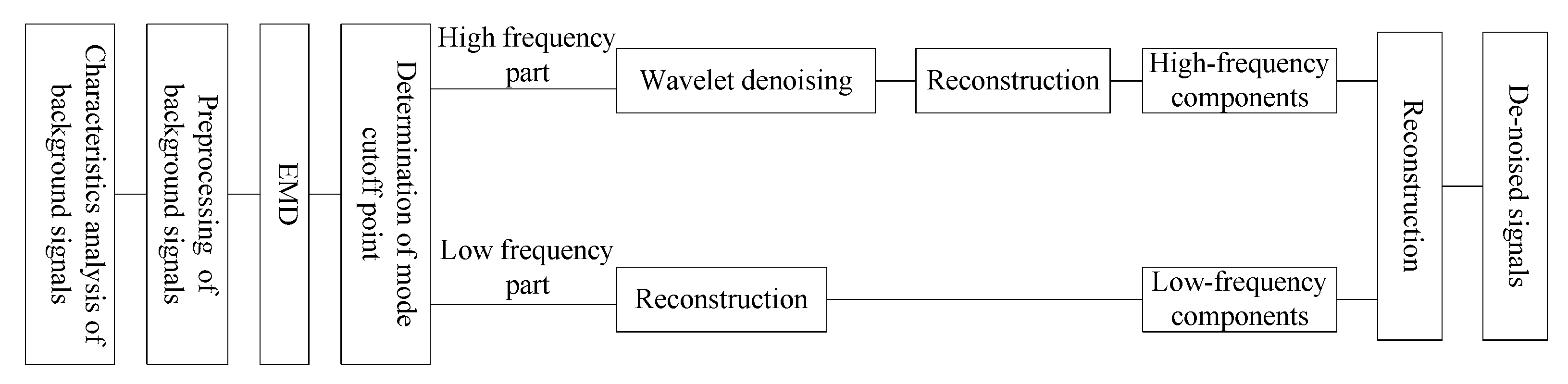
Due to the similarity of wavelet functions of Daubechies (db) and MS waves, db series wavelet bases are widely applied to the extraction of MS signals [48]. In this paper, db8 was used for the wavelet analysis of MS signals, and the decomposition scale was 4. The heuristic threshold principle and hard threshold filter method were adopted. Thus, the filtered signal and signal dominant modes could be reconstructed to achieve the denoised signal. The denoising process of signals is shown in Figure 4.

4. Results Analysis

4.1. Relationship of MS and Loading Force (F)

In this section, the relationship between MS and loading force (F) was analyzed by taking the change of raw coal specimens as an example. The relationship between MS and loading force of shaped and cement specimens was similar to that of raw coal specimens in general, which was not specified here. The differences between the three materials were highlighted in Section 5.2.2.

In six groups of raw coal specimens experiment, the coal specimens were all ruptured except in Exp.Y6. The peak force (F_max) and damage of coal specimens are shown in Table 1. Through the statistical analysis of the first five groups of experimental forces and MS signals, MS signals mainly concentrated in the fracture process (90–100% F_max) and after fracture. Therefore, we divided the signals of Exp.Y1–Exp.Y5 into eleven loading periods with 10% of the maximum force for an interval. The loading periods were respectively I (0–10%F_max), II (10–20%F_max), III (20–30%F_max), IV (30–40%F_max), V (40–50%F_max), VI (50–60%F_max), VII (60–70%F_max), VIII (70–80%F_max), IX (80–90%F_max), X (90–100%F_max) and XI (After F_max). Since the sample was not ruptured in Exp.Y6, it could not form a contrast to the other five experiments. Therefore, the paper did not divide the signals of Exp.Y6 into different periods. The relationship of MS and loading force (F) is shown in Figure 5.

As shown in Figure 5a–g, there were a certain number of MS signals in the early and middle loading stage of six experiments. However, the number of events was small and amplitude change was not evident. There was a quiet period approaching fracture. MS signals in the fracture process had the characteristics of dramatic changes of amplitude and event numbers.

Exp.Y4–Y6 adopted the multi-stage loading mode. There were several stages in which loading forces remained unchanged. It is shown in Figure 5f–h that there were not evident MS signals when the loading force remained unchanged in the low force state, for example in 140–170 s and 270–300 s of Figure 5g or 250–280 s of Figure 5h. While, there were obvious MS signals when the loading force remained unchanged in the high force state, such as 780–1065 s of Figure 5h. The results are similar to the previous studies on acoustic emission under constant load [49,50]. The phenomenon is associated with “creep” characteristics of coal materials. The internal damage of the coal sample in the low stress stage was small so that there was no visible MS signal. However, the internal damage was big in the high stress stage [51]. Although the stress remains constant, there was still crack propagation accompanied with the occurrence of many MS events.

4.2. MS Intensity Distribution Characteristics

Characteristic parameters of MS signal include the event count, event count rate, amplitude, energy count rate, etc. Moreover, intensity and frequency of the signal are usually reflected by the event count and amplitude. Event count was divided into the cumulative count and count rate. The threshold voltage of MS signal value could be set to 2 mv according to the statistical results of six experiments. The event count within each stress stage was counted by setting the threshold voltage value as 2 mv. Event count rate in each stage is shown in

Table 4. Event count rate of each stress stage in Exp.Y1–Exp.Y5. Note: “-” indicates the inexistence of the stage.

	I	II	III	IV	V	VI	VII	VIII	IX	X	XI
Exp.Y1	0.66	0.15	0.09	1.06	6.10	13.12	5.81	2.13	4.92	17.84	509.68
Exp.Y2	0.00	0.32	2.97	0.20	0.11	0.54	1.07	1.94	2.97	10.83	67.79
Exp.Y3	4.20	0.18	0.02	4.05	0.09	2.40	0.19	7.63	0.57	35.22	282.23
Exp.Y4	13.68	67.13	-	-	835.11	852.85	579.31	482.33	0.82	216.00	199.12
Exp.Y5	6.66	0.72	1.07	0.51	0.41	81.85	155.01	0.26	1.71	206.89	236.60

.

As shown in Table 4, the event count rate overally increased as the increase of the loading force. Event count rate was generally small in the early and middle loading stage, but increased greatly in the process of fracture and after fracture. MS signal intensity of each experiment was evaluated according to the event count rate and amplitude. The evaluation standard is shown in

Table 5. Signal strength evaluation standard.

		Amplitude (A)
		0 < A < 20 mv	A > 20 mv
Event count rate (R)	0 < R < 1	O	⬤
	1 < R < 10	⬤	⬤
	R >10	⬤	⬤

, in which O represents that the signal was not obvious, ⬤ represents that the signal was weaker, ⬤ represents that the signal was stronger and ⬤ represents that the signal was the strongest.

MS intensity distribution of each stress stage in Exp.Y1–Exp.Y5 is shown in

Table 6. MS intensity distribution of each stress stage. Note: “-” indicates inexistence of the stage.

	I	II	III	IV	V	VI	VII	VIII	IX	X	XI
Exp.Y1	⬤	O	O	⬤	⬤	⬤	⬤	⬤	⬤	⬤	⬤
Exp.Y2	O	O	⬤	O	O	O	⬤	⬤	⬤	⬤	⬤
Exp.Y3	O	O	O	O	O	O	⬤	⬤	O	⬤	⬤
Exp.Y4	⬤	⬤	-	-	⬤	⬤	⬤	⬤	O	⬤	⬤
Exp.Y5	⬤	⬤	⬤	O	O	⬤	⬤	O	O	⬤	⬤

according to the signal intensity evaluation standard.

4.3. MS Energy Evolution Characteristics

In order to analyze the characteristics of MS signals, the signals without obvious change during the six groups of experiments ere firstly intercepted, and the duration was taken as 1 s. After EMD decomposition of the intercepted signals, the energy percentages of each IMF component are calculated, as shown in

Table 7. Energy percentage of the signal without obvious change and noise (unit: %).

IMFn	Y1-1	Y1-2	Y2-1	Y2-2	Y3-1	Y3-2	Y4-1	Y4-2	Y5-1	Y5-2	Y6-1	Y6-2	Noise
1	60.20	60.4	51.80	54.20	62.00	62.70	63.40	64.10	65.10	66.70	61.50	63.20	67.80
2	21.30	21.1	19.90	20.30	17.10	22.60	17.00	17.70	17.90	17.40	19.10	18.80	17.10
3	9.02	9.05	12.10	11.50	8.46	8.05	8.92	8.75	8.70	8.06	8.52	8.02	7.93
4	4.66	4.55	6.41	6.82	5.25	3.42	4.43	4.37	4.76	4.34	5.91	5.50	3.55
5	2.58	2.63	3.46	3.49	2.93	1.54	2.90	2.87	1.90	1.81	2.36	2.25	1.85
6	0.93	0.98	2.53	2.66	2.72	0.63	1.10	1.08	0.80	0.82	1.05	1.05	0.89
7	0.49	0.48	1.07	0.54	0.81	0.62	0.68	0.69	0.36	0.50	0.89	0.66	0.45
8	0.37	0.42	1.00	0.26	0.62	0.24	0.26	0.20	0.18	0.20	0.43	0.44	0.33
9	0.29	0.19	0.97	0.12	0.02	0.07	1.09	0.22	0.05	0.06	0.16	0.05	0.06
10	0.11	0.19	0.67	0.10	0.01	0.05	0.14	0.01	0.03	0.06	0.05	0.02	0.03

. White noise signals with a sampling frequency of 2500 Hz and a length of 1 s were taken and EMD decomposition was also performed. After decomposition, the energy percentages of each IMF are also shown in Table 7.

Through the comparative analysis of the IMF energy percentage of signal without an obvious change and white noise signals (as shown in Figure 6), it could be found that the IMF energy percentage of the signal without obvious change had the same change trend with the white noise, which decreased at the exponential decay curve with the increase of decomposition layers, and the attenuation coefficient were 1.01 and 1.32. The energy of high-frequency component (IMF1–IMF2) accounted for about 80% of the total energy, but the energy of the low-frequency component (IMF3–IMF10) and residual were less than 20% of the total energy. It can be considered that when the change of collected signal is not distinct, there is no big difference between the IMF energy percentage change of collected signal and noise, and the main component of the collected signal is the noise dominant component.

The average frequency ($\stackrel{-}{f}$) of IMF of the signal without an obvious change and with an obvious change in the six groups of experiments was calculated, as shown in Figure 7. The average frequency decreased as the number of decomposition layers increased. The average frequency mainly changed in the form of the negative exponential attenuation of 2.

EMD was conducted in every stress stage with 1 s as an interval, and the average energy percentage of each IMF in every stress stage was counted. Statistical results are shown in Figure 8.

In contrast to Figure 5, Figure 8 and Table 6, the bigger the event count rate was, the less power percentage the low order IMF had and the more power percentage the high order IMF had. Moreover, the mode cutoff point distribution was closely related to the amplitude and event count rate, which performed the following laws.

(1)

The MS signal was not distinct or weak in the O stage or ⬤ stage. The IMF component energy percentage distribution was similar to the background noise, which was decreasing in the form of 2 to negative power. There was no distinct local energy minimum. The low order components (IMF1–IMF2) was still the main components of the signal, which accounted for 60–80% of the energy.

(2)

The MS signal was stronger in the ⬤ stage in which the IMF component energy percentage distribution was different from the background noise. The low order components (IMF1-2) energy percentage reduced and high order components (IMF3-10) energy percentage increased. Both of them were 40–60% of the energy and the former was a little higher than the latter. The order of the first local energy minimum was different in a different experiment, i.e., the orders were 3 in Exp.Y1 and Exp.Y2, 4 in Exp.Y4 or 7 in Exp.Y5.

The MS signal was the strongest in the ⬤ stage, which mostly occurred in the fracture process (X) and after fracture (XI). The energy percentages of IMF1 and IMF2 severely reduced to 20–40%, and the energy percentages of IMF3-10 were sharply increasing. There was a distinct local energy minimum. As shown in Figure 9, the orders of the first energy minimum were all 2 expect that was 3 in Exp.Y2. The event count rate of Exp.Y2 was much less than the other five experiments though the amplitude had no great difference with the other experiments (as shown in Figure 5 and Table 6), which resulted in the difference of the order of mode cutoff point between the Exp.Y2 and the other experiments. Thus, it could be seen that the order of mode cutoff point was determined both by the amplitude and event count rate.

Through the above analysis, there was an obvious cutoff point of the noise-dominant mode and signal-dominant mode in the fracture process under uniaxial compression, and the order of the cutoff point was 3. Namely, IMF1 and IMF2 were the noise-dominant mode, which contained more noise composition. The noise-dominant mode could be de-noised by means of wavelet threshold value and the reconstruction of de-noised signals was considered to be a useful high-frequency component. IMF3-10 was the signal-dominant mode, which contained less noise. The reconstruction of IMF3-10 was considered to be a useful low-frequency component.

The high-frequency modes IMF1–IMF2 were reconstructed by EMD and then were denoised by the wavelet threshold, thus the high-frequency component of MS signals could be obtained. While the low-frequency modes IMF3–IMF10 and the residual could be reconstructed directly through EMD to obtain the low-frequency component of the MS signals. In order to illustrate the shape of the signal after denoising, 1 s signal with obvious change in 89.5–90.5 s at the I stage and in 1172.0–1173.0 s at the XI stage were taken for example. The high-frequency and low-frequency components in 89.5–90.5 s at I stage and in 1172.0–1173.0 s at the XI stage are shown in Figure 10 and Figure 11 respectively. It could be found that the high-frequency component of the MS signals presented approximate exponential attenuation waveform characteristics, while the low-frequency component presented a “square wave” occurrence. In addition, the high-frequency component mainly reflected a fluctuation of MS signals and was related to the microcrack, while the low-frequency component represented the overall change trend of MS signals and mainly reflected the macro change of the crack.

4.4. Spectrum Evolution Law of MS Signals in the Deformation and Fracture of Coal and Rock Materials Under Load

Multiple IMF components c(t) can be obtained by the EMD method, and Hilbert transformation of each IMF can be expressed as:

$$H[c(t)]=\frac{1}{\pi }P.V.{\displaystyle {\int }_{-\infty }^{\infty }\frac{c(\tau )}{t-\tau }}d\tau$$

(8)

where, P.V. is the Cauchy principal value, thus constructing the analytic signal:

$$z(t)=c(t)+jH[c(t)]=a(t)e^{j\phi (t)}$$

(9)

where, $a(t)$ is amplitude function, $a(t)=\sqrt{c^2(t)+H^2[c(t)]}$, $\phi (t)$ is phase function and $\phi (t)=\arctan \frac{H[c(t)]}{c(t)}$.

The instantaneous frequency $\omega (t)$ $\omega (t)$ can be computed through the differential of the phase function.

$$\omega (t)=\frac{d\phi (t)}{dt}$$

(10)

Then the original signal can be expressed as:

$$f(t)=\mathrm{Re}{\displaystyle \sum _{m=1}^n{a}_m}(t)e^{i{\displaystyle \int {\omega }_m(t)dt}}$$

(11)

According to Formula (11), the signal amplitude, time and instantaneous frequency can be expressed in three-dimensional space, and then the Hilbert spectrum of signal can be obtained, which is expressed as:

$$H\left(\omega ,t\right)=\mathrm{Re}{\displaystyle \sum _{m=1}^n{a}_m\left(t\right)}{e}^{i{\displaystyle \int {\omega }_i\left(t\right)dt}}$$

(12)

Exp. Y1 was taken as an example to conduct the Hilbert power spectrum analysis of the high-frequency and low-frequency components of MS signals at 11 loading stages, and the results are shown in Figure 12 and Figure 13 respectively. The frequency spectrum of high-frequency and low-frequency components of MS signals in different loading stages of uniaxial compression presented the following characteristics.

(1)

When the stress was in 0–40% σ_c (I–V), the high-frequency component had the residual interference after denoising, and the power values were below 4. In the I stage, when the signal was evident, the power value of high-frequency component could reach 150 and the dominant frequency was 900 Hz. however, when the signal was not obvious, the power value was between 4 and 30, and the dominant frequency was between 300 and 400 Hz. By contrast, when the low-frequency component was stronger in the I and IV stage, the dominant frequency were 150–250 Hz, and when the low-frequency component was weak in the II and III stage, the signal was mainly the residual power-frequency interference.

(2)

When the stress reached 40–80% σ_c (V–VIII), the dominant frequency range of the high-frequency component firstly extended to 300–1000 Hz, then the range was getting narrow and were in 300–500 Hz. the power value reduced from 300 to 20 correspondingly. By contrast, low-frequency component changed significantly except in the VIII stage, the frequency was within 0–100 Hz, and the dominant frequency was in 0–30 Hz. The power value was bigger, and was between 3000 and 8000. In 70–80% σ_c (VIII) stage, the power values of high-frequency and low-frequency components were both smaller, and the signal was mainly the residual power-frequency interference. In this stage, MS signals were in the quiet period, and coal and rock materials were storing energy for the upcoming macro rupture.

(3)

When the stress was in the 80–100% σ_c (IX–X) stage, the frequency band of the high-frequency component became wider. Not only was the signal of 300–500 Hz distinct, but also the signal of 800–1000 Hz became evident. However, the dominant frequency of the low-frequency component remained in 0–30 Hz.

(4)

In the fracture stage (XI), the signals still had a large amplitude, and power values were larger. The frequency of the high-frequency component was 300–800 Hz, and that of the low-frequency component was 0–30 Hz. the power value of low-frequency component could reach about 5000, far more than the high-frequency component.

The above analysis shows that the frequency of MS signals induced by deformation and fracture of coal and rock was mainly 300–1000 Hz in the high-frequency component and 0–30 Hz in the low-frequency component. In addition, the main frequency of the signal was not fixed. With the increase of the stress, the power value of the low-frequency component was gradually higher than that of the high-frequency component, and the frequency of the MS signals was gradually transferred to the low frequency. Meanwhile, the change of frequency was closely related to the change of the signal amplitude.

5. Discussion

5.1. The Intrinsic Mechanism of Variation Characteristics of MS Signals

5.1.1. The MS Generation Mechanism of Coal and Rock Materials

MS is an energy released in the form of a stress wave induced by the crack generation, propagation and friction in the material, which is closely related to the deformation and failure in the local area of the material. Coal and rock materials are heterogeneous bodies composed of many tiny particles and pore fracture systems. Due to the existence of these pores and fractures, local deformation and fracture can be formed in coal and rock materials under the external load, which provides conditions for the generation of MS signals. Coal and rock material is a polycrystal composed of many grains, whose size can be smaller than micron or larger than centimeter. There are many cracks, pores and vacancies among them. The mechanical behavior of coal and rock materials is greatly affected by these defects. The deformation and fracture process of coal and rock can be divided into the following stages:

(1)

Closure stage of original microcrack. There are original microcracks in coal and rock materials, as shown in Figure 14a. At the beginning of the loading (I–III), when the stress reaches a certain degree, the larger original micro crack begins to close, and the crack begins to break off at the crack bifurcation point, as shown in Figure 14b. In this stage, MS is mainly generated by the fracture of microcrack, and the frequency is mostly of high-frequency.

(2)

New fracture formation and expansion stage. When the stress reaches the 30–60% of the peak stress level (IV–VI), the primary crack is compacted in the early stage, the characteristics of the coal and rock materials begin to show strong linear elastic and the MS signals are in the quiet period. While once the stress releases suddenly, there would be paroxysmal and relatively large-amplitude MS signals. The reason lies in that the deformation energy stored in the loaded coal and rock gradually increases with the increase of stress, and when the deformation reaches the expansion energy of the crack tip, the crack extension happens (as shown in Figure 14c) and release the elastic energy, which can produce strong MS signals. After the release of energy, the energy at the crack tip is not enough to cause the crack growth, and the crack growth will stop. Then the amplitude of MS signals returns to the normal value again, until the energy accumulates to the next crack growth process. At this stage, MS mainly comes from the formation and growth of the new crack.

(3)

Fracture confluence and connection stage. When the stress reaches 60–80% of the peak stress level (VII and VIII), coal and rock are in the condition of accelerating deformation, and large plastic deformation occurs. In the stage, the quantity of microcracks increases sharply, and a large number of microcracks propagate, converge and connect together (as shown in Figure 14d), thus obvious MS signals can be generated. The MS signals are caused by extrusion, friction and collision of crack surface in this stage.

(4)

Failure stage. At the stage of 80–100% peak stress (IX and X), coal and rock burst and develop failure (as shown in Figure 14e), and MS signals firstly experience a brief period of quiet, then the signal amplitude surges and stays in high status. This phenomenon illustrates that larger macro cracks are formed and coal and rock begin to failure. After peak stress (XI), macro cracks expand continuously, and change of MS signals is very distinct until the end of destruction.

The actual failure patterns of three kinds of coal and rock materials are shown in Figure 15. The failure mode of raw coal and cement specimens were mainly brittle failure, and longitudinal cracks propagated throughout the specimen, which are indicated in Figure 15a,c. The internal cracks were relatively developed, and the overall structure of the specimens was still relatively intact at the late stage of failure. However, the shaped coal specimens mainly collapsed along the longitudinal crack, and the internal crack were not developed, and the failure mode of shaped coal specimens was mainly plastic deformation, as shown in Figure 15b.

5.1.2. Correlation Model of Characteristic Parameters of MS and Damage

According to the continuum damage mechanics [52], the damage model of the material is established,

$$\sigma =E(1-D)\epsilon$$

(13)

where, E is elastic modulus; ε is the strain and D is the damage parameter. Under uniaxial stress, D represents the ratio of microcracks (micropores or microdefects) in the volume unit of the material. When D = 0, there is no damage in the material, and this is a reference state. When D = 1, the material is completely destroyed.

There is a close relationship between MS and the microfailure of coal and rock materials, and MS is the direct result of the deformation and failure of materials. Assuming that the fracture of each individual element contributes to MS, it can be considered that there is a proportional relationship between D and event count of MS. Tang et al. [53] confirmed that there was correspondence between stress wave and damage, and deduced the relationship between event count of MS and D:

$$D=\frac{N}{N_m}$$

(14)

where, N is the cumulative event count of MS monitored at any time and N_m is the cumulative event count of MS when coal and rock materials are completely destroyed.

For quasi-brittle materials (e.g., coal and rock), the damage law is often expressed by deformation variables such as strain, and it can be expressed as follows [54],

$$\mathrm{d}D=\{\begin{array}{ll}f(\epsilon )d\epsilon & (\epsilon \ge \zeta and d\epsilon >0)\\ 0& (\epsilon <\zeta and d\epsilon <0)\end{array}$$

(15)

where, f(ε) is continuous positive definite function ofε and can be called damage evolution function. ζ is a variable damage strain threshold.

It is assumed that the microelement strength of coal and rock materials obeys Weibull distribution, i.e.,

$$f(\epsilon )=\frac{n}{{\epsilon }_m}{(\frac{\epsilon }{{\epsilon }_m})}^{n-1}\exp [-{(\frac{\epsilon }{{\epsilon }_m})}^n]$$

(16)

where, n represents the homogeneity of coal and rock materials. The greater the value of n is, the more homogeneous the coal and rock materials are. ε_m is the reference mean strain when the stress reaches the peak stress. For monotone loading, the first equation in Formula (15) is always true. Assuming that the initial values of D, ε and ζ are all 0, through Formulas (14) and (16), the cumulative number of MS events can be represented as follows,

$$\frac{N}{N_m}=D={\displaystyle {\int }_0^{\epsilon }f(x)dx=1-\exp }[-{(\frac{\epsilon }{{\epsilon }_m})}^n]$$

(17)

Take the logarithm of both sides of Formula (17),

$$\ln (-\ln (1-\frac{N}{N_m}))=n\ln (\frac{\epsilon }{{\epsilon }_m})$$

(18)

According to Formula (17) or (18), the relationship between the event count (N) and the strain (ε) of raw coal, cement and shaped coal was analyzed respectively, as shown in Figure 16. It could be found that there were all good linear relationships between $\ln (-\ln (1-N/N_m))$ and $\ln (\epsilon /{\epsilon }_m)$ in the deformation and failure of three coal and rock materials. Therefore, the assumption that the microelement strength of coal and rock materials obeys Weibull distribution is correct. The n values in raw coal and cement experiment ranged from 2.35 to 3.03 and 4.66 to 6.18, respectively. However, for shaped coal reshaped by different particles, the n range was different for shaped coal of different particles, the range of n values depended on the size of particles. The fitting values of n values for particle sizes of less than 0.25 mm, 0.25–0.50 mm and 0.50~2.00 mm were 4.66–5.30, 3.98–5.06 and 3.65–4.48, respectively. With the increase of particle size, the homogeneity of materials decreased, and the corresponding n value decreased.

Statistical analysis of the range of n value in experiments of three materials is shown in Figure 17. It could be clearly seen that the n value of raw coal, shaped coal and cement sequentially increased, which indicates that the homogeneity of raw coal specimen was the lowest, that of briquette was the second and that of cement was the highest. The average values of n in the experiments of raw coal, shaped coal and cement were respectively 2.76, 4.51 and 6.57. The relationship between N/N_m and ε/ε_m in experiments of three materials is shown in Figure 18.

As seen in Figure 18, due to the relatively low homogeneity of raw coal and the development of defects such as microcracks or micropores, the event count of MS were obvious at the initial stage of loading stage, and the event count of MS signals of raw coal were higher than the other two materials before the main fracture. While the homogeneity of shaped coal and cement was relatively high, and internal defects such as microcracks or micropores were not developed, and MS signals were not obvious at the initial loading stage. The event count mainly focused on the late loading stage. The more homogeneous the material was, the less obvious the MS signals before main fracture.

5.1.3. The Intrinsic Reason of Spectrum Evolution of MS Signals

Through the analysis in Section 4.4, the frequency band of MS signals in coal and rock materials during the middle and late period of loading shows a trend of gradually widening. The frequency band of high-frequency component widened to 300–1000 Hz, and the frequency of low-frequency component was within 0–100 Hz. When approaching failure, there were more abundant low-frequency components than high-frequency components. Under the same MS monitoring sensor and monitoring system, the spectrum evolution law mainly depended on the source of MS and propagation medium.

There are many source mechanisms of MS, such as dislocation, plastic deformation and crack formation and propagation. The frequency spectrum of MS signals is determined by the duration of rapid unloading of MS source, i.e., energy release rate. The shorter the unloading duration is, the faster the energy release rate is, and the wider the spectrum of MS signals. Mirabile [55] insisted the MS source of coal and rock materials was dominated by crack formation and propagation, and calculated the energy released during the plastic deformation of the crack tip and the energy released during the crack propagation, which were respectively about 10⁻¹¹–10⁻⁷ J and 10⁻⁶–10⁻¹ J. Considering that the plastic deformation at the crack tip of low-brittle coal and rock is small and the released energy is correspondingly small, MS signals are mainly derived from crack propagation.

For brittle materials, Griffith argued that cracks could only begin to expand when the elastic energy released during the crack growth was equal to the plastic deformation energy and surface energy consumed during the crack growth [56]. The energy released during crack growth of the per unit area is defined as the energy release rate of crack growth, represented by G, and the energy consumed during crack growth of per unit area is represented by G_c. According to the energy balance relationship, the energy release rate criterion, i.e., Griffith fracture criterion is as follows,

$$G=G_c$$

(19)

That is, when G > G_c, the crack will lose its equilibrium and propagate; when G < G_c, the crack will not propagate and when G = G_c, the crack is in the critical state.

Under the condition of plane stress and mode-I crack, the fracture energy release rate G_I of brittle materials is

$$G_{\mathrm{I}}=\frac{K_{\mathrm{I}}^2}{E}$$

(20)

where, K_I is the stress intensity factor of mode-I crack and E is elastic modulus.

Meanwhile, for mode-I crack, the stress intensity factor $K_{\mathrm{I}}=\sigma \sqrt{\pi a}$, therefore,

$$G_{\mathrm{I}}=\frac{\pi a{\sigma }^2}{E}$$

(21)

where, a is half length of initial crack and $\sigma$ is normal stress.

Similarly, the fracture energy release rate of mode-II crack can be expressed as follows,

$$G_{\mathrm{II}}=\frac{K_{\mathrm{II}}^2}{E}=\frac{\pi a{\tau }^2}{E}$$

(22)

where, K_II is the stress intensity factor of mode-II crack and $\tau$ is shear stress.

The fracture energy release rate of mode-III crack can be expressed as follows,

$$G_{\mathrm{III}}=\frac{(1+\nu )K_{\mathrm{III}}^2}{E}=\frac{\pi (1+\nu )a{\tau }^2}{E}$$

(23)

where, K_III is the stress intensity factor of mode-III crack and $\nu$ is the Poisson’s ratio.

According to Formulas (21)–(23), with the increase of stress, the energy release rate increases, which can lead to the widening of MS signals spectrum. This was consistent with experimental results that the high-frequency and low-frequency signals both increased and the band width widened at the late loading stage.

As for the reason that the amplitude of low-frequency signal is higher than that of the high-frequency signal, it may be due to the influence of structure damage on the propagation and attenuation of MS signals. There are wave diffusion loss and internal friction loss in the process of MS propagation. The former has nothing to do with frequency, which is spherical wave attenuation in large solids and cylindrical wave attenuation in plates and the amplitude is inversely proportional to the propagation distance, while the amplitude of the latter is inversely proportional to the square of the propagation distance. Meanwhile, the higher the frequency of MS is, the greater the friction loss is. At the later loading stage, coal and rock damage increases, and macro cracks are formed and integrated accompanied by increase of internal friction loss during MS propagation. Thus, the loss of high-frequency MS signals is serious.

Furthermore, considering that all the specimens in the experiments are small specimens, the propagation distance of MS is short and the diffusion loss is small. Therefore, the loss of MS signals mainly lies in friction loss. For a MS event, multiple reflections of MS on the side and on the two end surfaces are superimposed to form multiple reflection waves with a long duration, which excite the natural vibration mode of the specimen, and enhance the vibration near natural frequency. This result in that the main frequency of the MS signals monitored actually is close to the natural spectrum of material.

In the uniaxial compression process of the specimens, due to the damage of the specimens, the structural stiffness will decrease correspondingly, and the natural frequency of specimens will also decrease correspondingly [57,58]. Thus, with the increase of specimen damage, the dominant frequency of MS detected by sensors installed on the surface of coal and rock materials is mainly low frequency. This is consistent with the experimental result.

5.2. Influencing Factors of MS Signals

5.2.1. Loading Rate

The amplitude, energy and cumulative energy of MS signals in the compression test of shaped coal and cement specimens were statistically calculated, and the corresponding analysis of these parameters and loading rate was conducted, as shown in Figure 19, Figure 20, Figure 21 and Figure 22, respectively. The amplitude of two channels of MS signals in shaped coal specimen experiment is of great discretization, and there is no evident law between the amplitude and loading rate. However, the energy and accumulative energy of MS signals in the shaped coal specimen experiment both decreased with the increase of the loading rate and were less affected by the particles. The amplitude of MS signals of cement specimen experiment was also discretized, but remained approximately the same and varied within a certain range. The energy and accumulative energy increased slightly with the increase of loading rate, but the magnitude of increase was small.

5.2.2. Composition and Structure of Specimen

The time-history curves of MS and stress in the experiment of shaped coal and cement are shown in Figure 23. Through comparative analysis of Figure 23 and Figure 5, it could be obtained that the amplitude of MS signals of cement specimen changed between −60 and 60 mV. The amplitude range was the same as that of raw coal, and the peak stress was an order of magnitude larger than that of raw coal. The change law of MS signals of cement specimen and raw coal specimen was similar in each stress loading period. However, the difference was that there was a very small amount of MS signals, and the amplitude was small at the early loading (I–III) stage of the cement specimen experiment. The reason was that composition particle size of cement specimens were in the μm grade, which was far less than the raw coal, and internal initial crack of cement specimens was less than raw coal, which resulting in that change of MS signals at the early loading (I–III) stage of the cement specimen experiment was not obvious.

In the deformation and fracture of shaped coal specimens, the amplitude of MS signals was relatively small, basically within −6–6 mV, and the peak stress was an order of magnitude smaller than that of raw coal. In the loading stage (I–VI), the change law of MS signals of shaped coal and raw coal was the same, and when the stress was in the 60–90% peak stress level (VII–IX), MS signals were in the abnormal quiet period, and signal amplitude did not significantly change. Only 100% (X) of peak stress and after the peak stress (XI) began did MS change significantly. In addition, MS signals greatly lagged behind the change of stress, which was largely different from that of raw coal. The possible reason is that the production process of shaped coal specimens had changed the complex structure of the original coal and rock materials, and the shaped coal specimens had better homogeneity and fewer internal defects. In addition, the experimental loading rate was relatively slow, which was similar to the rheological process. The above two reasons together caused the MS signals in shaped coal specimens experiment to not be obvious.

The amplitude, energy and cumulative energy of MS signals of raw coal, shaped coal and cement were calculated, as shown in Figure 24 and Figure 25. The difference between the signal amplitude of raw coal and cement specimens was small, both of which were higher than that of shaped coal. However, the energy and the cumulative energy of MS signals of raw coal specimens were both larger than that of shaped coal and cement specimens, and the signal amplitude of shaped coal and cement were roughly the same. It seemed that the main reason for the difference in MS signals also lay in the influence of fractures, pores, joint bedding and other structures. Raw coal contains many of the above-mentioned structures with weak surface and sufficient crack growth conditions. Although the compressive strength was low, the MS signals in raw coal were very rich and the signal changes were evident. However, the particles in shaped coal and cement specimens were broken to a small extent. Under compression, the particles themselves were difficult to be destroyed, and the internal initial crack was less and difficult to expand. Only when the stress reached a certain level and the specimen was subjected to tensile failure were there obvious MS signals.

In conclusion, the generation of MS signals was related to the stress, load mode and microstructure of coal and rock. The properties of coal and rock, such as strength, development degree of original fracture, particle size and dense degree had a decisive influence on the amplitude, frequency, energy and other characteristic parameters of MS signals. While the relationship between the change of MS parameters and loading rate was not strong.

5.3. Prediction Method of Deformation and Failure of Coal and Rock Based on MS Spectrum Evolution

5.3.1. Determination Method of the Energy Ratio of Low and High-Frequency Components (EL/EH)

Through the above analysis, with the increase of coal and rock damage, the frequency band of MS widened, and the amplitude of low-frequency signal was significantly higher than the high-frequency signal when approaching failure. Thus, the ratio of low-frequency and high-frequency energy components (EL/EH) of MS signals could be a sign of damage. The energy ratio of low-frequency and high-frequency components of Exp. Y1 is shown in Figure 26. It could be found that EL/EH in the raw coal experiment presented the characteristics of “quiet-growth-shortly quiet-growth”. In early loading (I–III), the MS was mainly the high-frequency signal, EL/EH changed within the range of 0–5. When the stress reached 30–60% of the peak stress level (IV–VI), new micro cracks were formed and propagated. Once stress released suddenly, paroxysmal MS signals with relatively large amplitude were generated and the low-frequency signal increased greatly, EL/EH presented paroxysmal growth and changes were within 5–15. When the stress was in 60–80% of peak stress (VII and VIII), micro cracks quantity increased sharply, a large number of microcracks propagated and converged and connected together, which produced a significant high-frequency signal, while a low-frequency signal was not evident. Thus, a short quiet period appeared for EL/EH. Compared to the first quiet period, the value of EL/EH was slightly bigger, which changed within the range of 0–10. At the 80–100% peak stress stage (IX and X), coal and rock burst and developed failure. Meanwhile, the larger macro cracks developed, and the low-frequency signal was greatly distinct, there would be a continuous growth of EL/EH, until the end of destruction.

Therefore, EL/EH increased along with the increase of stress in the deformation and fracture of coal and rock materials, and the energy ratio (EL/EH) could be used to characterize the process of deformation and fracture of coal and rock. EL/EH presented the trend of “quiet-growth-shortly quiet-growth” under the condition of experiment. When there was a trend of “growth-shortly quiet-growth”, and EL/EH was more than 10, an early warning could be in effect. However, EL/EH determination method could only determine the general trend of instability failure of coal and rock, and could not accurately determine the time of instability failure. In order to solve this problem, it could be supplemented by the cumulative energy prediction method.

5.3.2. A Method to Determine the Instability Failure Time of Coal and Rock Materials Based on Cumulative Energy

The comparative analysis of the cumulative energy of MS signals and pressure in raw coal and cement specimens experiments is shown in Figure 27. The sudden decrease and increase of the load force in raw coal experiments also led to the increase of MS signals. After the force exceeded the peak force, the release of MS signals was accelerated, as shown in Figure 27a. The relationship between MS signals and force in experiments of cement specimens was very similar to that of raw coal. After the force exceeded the peak force, the change of MS signal lagged behind the change of force, but the lag was not distinct, as shown in Figure 27b.

According to the above analysis, the cumulative energy value of MS signals had an accelerated release process of energy when approaching the failure, which corresponded to a critical point of the energy value. Vere-jones [59] put forward the theory of energy critical point, and then a large number of researchers adopted different mathematical models to study the accelerated release process of energy, and gradually formed the theory of energy-accelerated release. The research results showed that the initial determination formula of the energy critical point was the power-law formula, namely,

$$W(t)=a+b{(t_c-t)}^d$$

(24)

where, $W(t)$ is signal energy, a, b and d are all constant, $t_c$ is the critical moment of rupture and d reflects the release speed of energy. As can be seen from the Formula (24), the smaller the value of d is, the faster the release speed of energy is and the more dangerous the state of the system is.

In addition, Mignan [60] considered that energy value of materials might fluctuate slightly when approaching failure. After revising Formula (24), the Log Periodic Power Law (LPPL) model was proposed, which was as follows,

$$W(t)=a+b{(t_c-t)}^d+c{(t_c-t)}^d\cos (\omega \ln (t_c-t)+\phi )$$

(25)

where, c is a constant, $\omega$ is the angular frequency and $\phi$ is the phase.

Considering that there is an accelerated release phase of MS signals energy when coal and rock materials are approaching the failure, the LPPL fitting result of cumulative energy of MS in Exp. Y1 is shown in Figure 28. It can be seen that the LPPL model had a good fitting effect, and the rupture time inferred from MS was estimated to be 1214.5 s. The cumulative energy prediction method could effectively make up the shortcomings of EL/EH prediction method and could predict the time point of instability failure of coal and rock. In conclusion, the combination of the cumulative energy prediction method and the EL/EH prediction method could effectively realize the monitoring and early warning of the deformation and fracture of coal and rock materials.

6. Conclusions

By changing loading modes (constant speed, variable speed and graded loading) and physical properties of coal and rock (strength, components and grain size), synchronous analysis of deformation and failure process of coal and rock materials and the time-frequency evolution process of MS signals was conducted. The influence of factors, such as load mode, load stage and grain size and strength of coal and rock materials and weak structure surface, on MS signals was analyzed. The spectrum evolution of MS signals in the process of the deformation and failure of coal and rock materials was obtained. The main conclusions were as follows,

(1)

A certain number of MS signals were generated in the early and middle stage of compression loading of coal and rock, but the amplitude change was not distinct. There was a quiet period before the adjacent rupture, and the amplitude of MS signals would change sharply and last for a short time during the rupture. After fracture, there were still strong MS signals. When the pressure remained unchanged, the coal and rock materials also produced MS signals under high pressure stress. This phenomenon might be related to the “creep” characteristic of coal and rock materials.

(2)

According to statistical analysis of the energy changes of each IMF component of MS signals after EMD decomposition, it was concluded that there was an evident cutoff point between the dominant mode of noise and the dominant mode of MS signals in the process of coal and rock rupture, and the cutoff point was 3. The MS signals could be well denoised using HHT and wavelet threshold methods. In addition, the high-frequency component of the MS signals presented approximate exponential attenuation waveform characteristics, while the low-frequency component presented a “square wave” occurrence.

(3)

The frequency spectrum of the high-frequency component of MS signals was rich, distributed in 300–1200 Hz, the frequency spectrum of low-frequency component was distributed at 0–200 Hz and the frequency spectrum of the low-frequency component of MS signals near and after rupture was mainly distributed at 0–30 Hz. The high-frequency component reflected the fluctuation of MS signals, which was related to the micro fracture degree in the coal and rock materials, while the low-frequency component reflected the overall trend of MS signals, which was related to the macro fracture degree in the coal and rock materials. The spectrum evolution law mainly depended on the source of MS and the propagation medium. With the increase of damage, the energy release rate increased, which could lead to the widening of MS signals spectrum. While the stiffness and natural frequency of specimens decreased correspondingly, and friction loss and resonance effect caused that the dominant frequency of MS detected by sensors installed on the surface of coal and rock materials was mainly of low frequency.

(4)

The relationship between the change of MS parameters, such as the amplitude, energy and cumulative energy and loading rate had no obvious regularity. The amplitude of the MS signals generated by the raw coal specimens was approximately equal to that of the cement specimens, both of which were higher than the shaped coal specimens. In terms of energy and cumulative energy, raw coal was greatly higher than shaped coal and cement specimens. The energy ratio (EL/EH) could be used to characterize the process of deformation and fracture of coal and rock. EL/EH presented the trend of “quiet-growth-shortly quiet-growth” under the condition of experiment. When there was a trend of “growth-shortly quiet-growth”, and EL/EH was more than 10, an early warning could be in effect. Besides, the combination of cumulative energy prediction method and EL/EH prediction method could effectively realize the monitoring and early warning of deformation and fracture of coal and rock. In all, the spectrum and energy evolution of MS signals could be used as a characterization method of the degree of damage of coal and rock materials.

(5)

Due to the limitations of test conditions and defect of experimental design idea, the research on MS event locations or source mechanisms was not getting enough attention. In future work, we will use CT Imaging technology, SEM, high-speed photography or other related technology and a numerical simulation method to carry out relevant research on MS event locations or source mechanisms on the basis of existing research. Through a better understanding of where the MS events are located and how the actual failure occurs, the experimental phenomenon, MS generation mechanism of coal and rock materials, correlation model of characteristic parameters of MS and damage and prediction method can get a better explanation and validation.

References

1. Chlebowski, D.; Zorychta, A.; Burtan, Z.; Cała, M. Location of opening-out cross-cuts in relation to rockburst hazard conditions along the face in the light of model testing. Arch. Min. Sci. 2017, 62, 121–130. [Google Scholar] [CrossRef] [Green Version]
2. Sainoki, A.; Emad, M.Z.; Mitri, H.S. Study on the efficiency of destress blasting in deep mine drift development. Can. Geotech. J. 2017, 54, 518–528. [Google Scholar] [CrossRef] [Green Version]
3. Diekmann, L.; Schwarz, B.; Bauer, A.; Gajewski, D. Source localization and joint velocity model building using wavefront attributes. Geophys. J. Int. 2019, 219, 995–1007. [Google Scholar] [CrossRef]
4. Ma, C.; Jiang, Y.; Li, T. Gravitational Search Algorithm for Microseismic Source Location in Tunneling: Performance Analysis and Engineering Case Study. Rock Mech. Rock Eng. 2019, 52, 3999–4016. [Google Scholar] [CrossRef]
5. Li, A.; Zhang, D.; Fang, Q.; Luo, J.; Gao, L.; Sun, Z. Safety Distance of Shotcrete Subjected to Blasting Vibration in Large-Span High-Speed Railway Tunnels. Shock Vib. 2019, 2019, 1–14. [Google Scholar] [CrossRef] [Green Version]
6. Li, B.; Xu, N.; Dai, F.; Zhang, G.; Xiao, P. Dynamic analysis of rock mass deformation in large underground caverns considering microseismic data. Int. J. Rock Mech. Min. Sci. 2019, 122, 104078. [Google Scholar] [CrossRef]
7. Zhao, Y.; Yang, T.; Zhang, P.; Xu, H.; Zhou, J.; Yu, Q. Method for Generating a Discrete Fracture Network from Microseismic Data and its Application in Analyzing the Permeability of Rock Masses: A Case Study. Rock Mech. Rock Eng. 2019, 52, 3133–3155. [Google Scholar] [CrossRef]
8. Zhu, Q.; Li, Q.; Feng, Y.; Heng, X.; Li, S.; Yang, T. An Experimental Investigation on the Relationship between MS Frequency Response and Coal and Gas Outburst. Shock Vib. 2018, 2018, 1–13. [Google Scholar] [CrossRef]
9. Ding, Y.; Dou, L.; Cai, W.; Chen, J.; Kong, Y.; Su, Z.; Li, Z. Signal characteristics of coal and rock dynamics with micro-seismic monitoring technique. Int. J. Min. Sci. Technol. 2016, 26, 683–690. [Google Scholar] [CrossRef]
10. Wang, X.; Yu, S.; Yin, D. Time-frequency Characteristics of Micro-seismic Signals Before and after Rock Burst. In Proceedings of the 9th China-Russia Symposium” Coal in the 21st Century: Mining, Intelligent Equipment and Environment Protection” (COAL 2018), Qingdao, China, 18–21 October 2018; Atlantis Press: Paris, France, 2018. [Google Scholar]
11. He, X.; Wang, A.; Dou, L.; Song, D.; Zu, Z.; Li, Z. Technology of microseismic dynamic monitoring on coal and gas outburst—Prone zone. J. China Coal Soc. 2018, 43, 3122–3129. (In Chinese) [Google Scholar]
12. Zhu, Q.; Jiang, F.; Wei, Q.; Wang, B.; Liu, J.; Liu, X. An automatic method determining arrival times of microseismic P-phase in hydraulic fracturing of coal seam. Chin. J. Rock Mech. Eng. 2018, 37, 2319–2333. [Google Scholar]
13. Maity, D.; Ciezobka, J. Using microseismic frequency-magnitude distributions from hydraulic fracturing as an incremental tool for fracture completion diagnostics. J. Pet. Sci. Eng. 2019, 176, 1135–1151. [Google Scholar] [CrossRef]
14. Chen, H.; Meng, X.; Niu, F.; Tang, Y.; Yin, C.; Wu, F. Microseismic monitoring of stimulating shale gas reservoir in SW China: 2. Spatial clustering controlled by the preexisting faults and fractures. J. Geophys. Res. Solid Earth 2018, 123, 1659–1672. [Google Scholar] [CrossRef] [Green Version]
15. Martínez-Garzón, P.; Bohnhoff, M.; Kwiatek, G.; Zambrano-Narváez, G.; Chalaturnyk, R. Microseismic monitoring of CO2 injection at the penn west enhanced oil recovery pilot project, Canada: Implications for detection of wellbore leakage. Sensors 2013, 13, 11522–11538. [Google Scholar] [CrossRef] [PubMed] [Green Version]
16. Mao, H.; Xu, N.; Li, B.; Fan, Y.; Wu, J.; Meng, G. Stability analysis of the left bank underground powerhouse of Baihetan Hydropower Station based on discrete element simulation and microseismic monitoring. Rock Soil Mech. 2020, 41, 1–15. (In Chinese) [Google Scholar]
17. Ma, T.; Tang, C.; Tang, L.; Zhang, W.; Wang, L. Mechanism of rock burst forcasting based on micro-seismic monitoring technology. Chin. J. Rock Mech. Eng. 2016, 35, 470–483. (In Chinese) [Google Scholar]
18. Dai, F.; Li, B.; Xu, N.; Fan, Y.; Xu, J.; Liu, J. Microseismic characteristic analysis of underground powerhouse at Baihetan hydropower station subjected to excavation. Chin. J. Rock Mech. Eng. 2016, 35, 692–703. (In Chinese) [Google Scholar]
19. Xu, N.W.; Dai, F.; Liang, Z.Z.; Zhou, Z.; Sha, C.; Tang, C.A. The dynamic evaluation of rock slope stability considering the effects of microseismic damage. Rock Mech. Rock Eng. 2014, 47, 621–642. [Google Scholar] [CrossRef]
20. Nadeau, R.M.; McEvilly, T.V. Fault slip rates at depth from recurrence intervals of repeating microearthquakes. Science 1999, 285, 718–721. [Google Scholar] [CrossRef] [Green Version]
21. Eaton, D.W.; Igonin, N.; Poulin, A.; Weir, R.; Zhang, H.; Pellegrino, S.; Rodriguez, G. Induced seismicity characterization during hydraulic-fracture monitoring with a shallow-wellbore geophone array and broadband sensors. Seismol. Res. Lett. 2018, 89, 1641–1651. [Google Scholar] [CrossRef]
22. Lachaud, C.; Marsan, D.; Montagnat, M.; Weiss, J.; Moreau, L.; Gimbert, F. Micro-seismic monitoring of a shear fault within a floating ice plate. J. Geophys. Res. Solid Earth 2019, 124, 10444–10467. [Google Scholar] [CrossRef]
23. Lherminier, S.; Planet, R.; dit Vehel, V.L.; Simon, G.; Vanel, L.; Måløy, K.J.; Ramos, O. Continuously sheared granular matter reproduces in detail seismicity laws. Phys. Rev. Lett. 2019, 122, 218501. [Google Scholar] [CrossRef] [PubMed] [Green Version]
24. Blake, W.; Leighton, F.W.; Duvall, W.I. Microseismic Techniques for Monitoring the Behavior of Rock Structures; US Department of the Interior, Bureau of Mines: Washington, DC, USA, 1974.
25. Lu, C.P.; Liu, G.J.; Liu, Y.; Zhang, H. Mechanisms of Rockburst Triggered by Slip and Fracture of Coal-Parting-Coal Structure Discontinuities. Rock Mech. Rock Eng. 2019, 52, 3279–3292. [Google Scholar] [CrossRef]
26. Ma, K.; Yuan, F.; Zhuang, D.; Li, Q.; Wang, Z. Study on Rules of Fault Stress Variation Based on Microseismic Monitoring and Numerical Simulation at the Working Face in the Dongjiahe Coal Mine. Shock Vib. 2019, 2019, 1–12. [Google Scholar] [CrossRef] [Green Version]
27. Xia, Y.X.; Lan, H.; Mao, D.B.; Pan, J.F. Study of the lead abutment pressure distribution base on microseismic monitoring. J. China Univ. Min. Technol. 2011, 40, 868–873. (In Chinese) [Google Scholar]
28. He, J.; Dou, L.; Gong, S.; Li, J.; Ma, Z. Rock burst assessment and prediction by dynamic and static stress analysis based on micro-seismic monitoring. Int. J. Rock Mech. Min. Sci. 2017, 100, 46–53. [Google Scholar] [CrossRef]
29. Wu, A.X.; Wu, L.C.; Liu, X.H.; Wang, C.L.; Huang, W.S.; Zhu, Q.J. Space-time distribution of microseismic activities in mines. J. Univ. Sci. Technol. Beijing 2012, 34, 609–613. (In Chinese) [Google Scholar]
30. Kwiatek, G.; Goebel, T.H.W.; Dresen, G. Seismic moment tensor and b value variations over successive seismic cycles in laboratory stick-slip experiments. Geophys. Res. Lett. 2014, 41, 5838–5846. [Google Scholar] [CrossRef] [Green Version]
31. Chen, X.; Li, W.; Yan, X. Analysis on rock burst danger when fully-mechanized caving coal face passed fault with deep mining. Saf. Sci. 2012, 50, 645–648. [Google Scholar] [CrossRef]
32. Ge, M. Efficient mine microseismic monitoring. Int. J. Coal Geol. 2005, 64, 44–56. [Google Scholar] [CrossRef]
33. Errington, A.F.C.; Daku, B.L.F.; Prugger, A.F.; Dodds, D.E. Energy spectral density characterization of microseismic events in potash mines. Measurement 2009, 42, 264–268. [Google Scholar] [CrossRef]
34. Lu, C.P.; Dou, L.M.; Liu, B.; Xie, Y.S.; Liu, H.S. Microseismic low-frequency precursor effect of bursting failure of coal and rock. J. Appl. Geophys. 2012, 79, 55–63. [Google Scholar] [CrossRef]
35. Li, C.; Liu, J.; Wang, C.; Li, J.; Zhang, H. Spectrum characteristics analysis of microseismic signals transmitting between coal bedding. Saf. Sci. 2012, 50, 761–767. [Google Scholar] [CrossRef]
36. Yuan, R.; Li, H.; Li, H.Z. Distribution of microseismic signal and discrimination of portentous information of pillar type rockburst. Chin. J. Rock Mech. Eng. 2012, 31, 80–85. (In Chinese) [Google Scholar]
37. Capilla, C. Application of the Haar wavelet transform to detect microseismic signal arrivals. J. Appl. Geophys. 2006, 59, 36–46. [Google Scholar] [CrossRef]
38. Zhu, Q.; Jiang, F.; Yu, Z.; Yin, Y.; Lu, L. Study on energy distribution characters about blasting vibration and rock fracture microseismic signal. Chin. J. Rock Mech. Eng. 2012, 31, 723–730. (In Chinese) [Google Scholar]
39. Kizhner, S.; Flatley, T.P.; Huang, N.E.; Blank, K.; Conwell, E. On the Hilbert-Huang transform data processing system development. In Proceedings of the IEEE Aerospace Conference Proceedings (IEEE Cat. No. 04TH8720), Big Sky, MT, USA, 6–13 March 2004; IEEE: Piscataway, NJ, USA, 2004; Volume 3, pp. 1961–1979. [Google Scholar]
40. Wang, Q.; Li, C.; Lyu, P.; Zhao, Y.; Ai, D.; Xie, B. Experimental Study on Stress Evolution and Microseismic Signals under Vibration Conditions of Coal during Excavation and Subsequent Waiting Time. Shock Vib. 2019, 2019, 1–13. [Google Scholar] [CrossRef] [Green Version]
41. Bieniawski, Z.T.; Bernede, M.J. Suggested methods for determining the uniaxial compressive strength and deformability of rock materials. Int. J. Rock Mech. Min. Sci. Geomech. Abstr. 1979, 16, 138–140. [Google Scholar] [CrossRef]
42. Dudley, J.W.; Brignoli, M.; Crawford, B.R.; Ewy, R.T.; Love, D.K.; McLennan, J.D.; Ramos, G.G.; Shafer, J.L.; Sharf-Aldin, M.H.; Siebrits, E.; et al. ISRM suggested method for uniaxial-strain compressibility testing for reservoir geomechanics. Rock Mech. Rock Eng. 2016, 49, 4153–4178. [Google Scholar] [CrossRef]
43. General Administration of Quality Supervision, Inspection and Quarantine of the People’s Republic of China; China National Standardization Management Committee. GB 474–2008, The Preparation Method of Coal Sample; China Standards Press: Beijing, China, 2008. (In Chinese)
44. Ministry of Housing and Urban-Rural Development of the People’s Republic of China; State Administration for Market Regulation. GBT2050081–2019, Standard Test Methods for Physical and Mechanical Properties of Concrete; China Building Industry Press: Beijing, China, 2019. (In Chinese)
45. Huang, N.E.; Shen, Z.; Long, S.R.; Wu, M.C.; Shih, H.H.; Zheng, Q.A.; Yen, N.; Tung, C.C.; Liu, H.H. The empirical mode decomposition and the Hilbert spectrum for nonlinear and non-stationary time series analysis. Proc. R. Soc. Lond. Ser. A Math. Phys. Eng. Sci. 1998, 454, 903–995. [Google Scholar] [CrossRef]
46. Boudraa, A.O.; Cexus, J.C. EMD-based signal filtering. IEEE Trans. Instrum. Meas. 2007, 56, 2196–2202. [Google Scholar] [CrossRef]
47. Sun, W.; Peng, Y.; Xu, J. A de-noising method for laser ultrasonic signal based on EMD. J. Shandong Univ. (Eng. Sci.) 2008, 38, 121–126. (In Chinese) [Google Scholar]
48. Xie, J.; Wen, Z.; Li, X.; Li, Y.; Lu, H.; Huang, J. Analysis of velocity pulses for near-fault strong motions from the Wenchuan earthquake based on wavelet method. Chin. J. Geophys. 2012, 55, 1963–1972. (In Chinese) [Google Scholar]
49. Shen, B.; Stephansson, O.; Rinne, M. Introduction to Rock Fracture Mechanics. In Modelling Rock Fracturing Processes; Springer: Dordrecht, The Netherlands, 2014. [Google Scholar]
50. Li, N.; Wang, E.Y.; Zhao, E.L.; Ma, Y.K.; Xu, F.L.; Qian, W.H. Experiment on acoustic emission of rock damage and fracture under cyclic loading and multi-stage loading. J. China Coal Soc. 2010, 35, 1099–1103. (In Chinese) [Google Scholar]
51. Flandrin, P.; Rilling, G.; Goncalves, P. Empirical mode decomposition as a filter bank. IEEE Signal Process. Lett. 2004, 11, 112–114. [Google Scholar] [CrossRef] [Green Version]
52. Rabotnov, Y.N. Paper 68: On the equation of state of creep. In Proceedings of the Institution of Mechanical Engineers, Conference Proceedings, London, UK, 1 June 1963; SAGE Publications: London, UK, 1963; Volume 178, pp. 2-117–2-122. [Google Scholar]
53. Tang, C.A.; Xu, X.H. Evolution and propagation of material defects and Kaiser effect function. J. Seismol. Res. 1990, 13, 203–213. [Google Scholar]
54. Mazars, J. Mechanical damage and fracture of concrete structures. In Advance in Fracture Research, Proceedings of the 5th International Conference on Fracture, Cannes, France, 29 March–3 April 1981; François, D., Ed.; Oxford Pergamon Press: Oxford, UK, 1981; pp. 499–506. [Google Scholar]
55. Mirabile, M. Acoustic emission energy and mechanisms of plastic deformation and fracture. Non Destr. Test. 1975, 8, 77–84. [Google Scholar] [CrossRef]
56. Grriffith, A.A. The phenomenon of rupture and flow in solids. Philos. Trans. R. Soc. Ser. A 1920, 1920221, 163–197. [Google Scholar]
57. Lee, J.W. Crack identification method for tapered cantilever pipe-type beam using natural frequencies. Int. J. Steel Struct. 2016, 16, 467–476. [Google Scholar] [CrossRef]
58. Dilena, M.; Dell’Oste, M.F.; Morassi, A. Detecting cracks in pipes filled with fluid from changes in natural frequencies. Mech. Syst. Signal Process. 2011, 25, 3186–3197. [Google Scholar] [CrossRef]
59. Vere-Jones, D. Statistical theories of crack propagation. J. Int. Assoc. Math. Geol. 1977, 9, 455–481. [Google Scholar] [CrossRef]
60. Mignan, A. Retrospective on the Accelerating Seismic Release (ASR) hypothesis: Controversy and new horizons. Tectonophysics 2011, 505, 1–16. [Google Scholar] [CrossRef]
Figure 1. Coal and rock specimens. (a) Raw coal; (b) shaped coal specimens and (c) cement specimens.
Energies 13 00809 g001
Figure 2. The diagram of the microseismic (MS) test system under uniaxial compression.
Energies 13 00809 g002
Figure 3. The test apparatus and arrangement of MS sensors.
Energies 13 00809 g003
Figure 4. The denoising process of signals.
Energies 13 00809 g004
Figure 5. The relationship of MS and loading force (F). (a) Exp.Y1-1; (b) Exp.Y1-2; (c) Exp.Y2-1; (d) Exp.Y2-2; (e) Exp.Y3-1; (f) Exp.Y4-1; (g) Exp.Y5-1 and (h) Exp.Y6-1. Note: Exp.Y1-1 represents the 1# MS sensor of experiment Y1, and Exp.Y1-2 represents the 2# MS sensor of experiment Y1, similarly hereinafter.
Energies 13 00809 g005
Figure 6. Contrast of the energy percentage of the signal without obvious change and noise. (a) Signal without an obvious change and (b) white noise. For the label of horizontal axis, IMFn represents respectively IMF1, IMF2, IMF3, …, IMF10.
Energies 13 00809 g006
Figure 7. Average frequency ( f ) of each IMFn. (a) Signal without an obvious change and (b) signal with an obvious change.
Energies 13 00809 g007
Figure 8. Intrinsic mode function (IMF) energy distribution graph of each load stage in Exp.Y1–Y5. (a) Exp.Y1; (b) Exp.Y2; (c) Exp.Y3; (d) Exp.Y4 and (e) Exp.Y5.
Energies 13 00809 g008
Figure 9. IMF energy percentage graph in the fracture process (X) and after a fracture (XI).
Energies 13 00809 g009
Figure 10. High-frequency and low-frequency components of MS in 89.5–90.5 s at the I stage. (a) High-frequency component and (b) low-frequency component.
Energies 13 00809 g010
Figure 11. High-frequency and low-frequency components of MS in 1172.0–1173.0 s at the XI stage. (a) High-frequency component and (b) low-frequency component.
Energies 13 00809 g011
Figure 12. Hilbert power spectrum of the high-frequency component of MS at loading stages I–XI in Exp. Y1. Note: the left part is the Hilbert power spectrum, and the right part is the power-frequency diagram. The power in the Figure 12 is dimensionless, which represents the possibility of the signal in a specific time and frequency.
Energies 13 00809 g012aEnergies 13 00809 g012bEnergies 13 00809 g012c
Figure 13. Hilbert power spectrum of the low-frequency component of MS at loading stages I–XI in Exp. Y1. Note: the left part is the Hilbert power spectrum, and the right part is the power-frequency diagram. The power in the Figure 13 is dimensionless, which represents the possibility of the signal in a specific time and frequency.
Energies 13 00809 g013aEnergies 13 00809 g013bEnergies 13 00809 g013c
Figure 14. The deformation and failure process of coal and rock materials. (a) Original state; (b) closure stage; (c) new fracture formation and expansion stage; (d) fracture confluence and connection stage and (e) failure stage.
Energies 13 00809 g014
Figure 15. Failure forms of three coal and rock materials. (a) Raw coal; (b) shaped coal and (c) cement.
Energies 13 00809 g015
Figure 16. The fitting relationship between ln ( ln ( 1 N / N m ) ) and ln ( ε / ε m ) in experiments of three materials. (a) Raw coal; (b) cement; (c) shaped coal (less than 0.25 mm); (d) shaped coal (0.25–0.50 mm) and (e) shaped coal (0.50–2.00 mm).
Energies 13 00809 g016
Figure 17. Fitting values of n for three coal and rock materials.
Energies 13 00809 g017
Figure 18. The relationship between N/Nm and ε/εm.
Energies 13 00809 g018
Figure 19. 1# MS sensors of shaped coal.
Energies 13 00809 g019
Figure 20. 2# MS sensors of shaped coal.
Energies 13 00809 g020
Figure 21. 1# MS sensors of cement specimens.
Energies 13 00809 g021
Figure 22. 2# MS sensors of cement specimens.
Energies 13 00809 g022
Figure 23. MS and loading force (F) of shaped coal and cement specimens. (a) Shaped coal and (b) cement.
Energies 13 00809 g023
Figure 24. Amplitude, energy and cumulative energy of 1# MS sensors.
Energies 13 00809 g024
Figure 25. Amplitude, energy and cumulative energy of 2# MS sensors.
Energies 13 00809 g025
Figure 26. Energy ratio of low-frequency and high-frequency components in Exp. Y1.
Energies 13 00809 g026
Figure 27. Accumulative value of MS signals and loading force (F) in experiments of raw coal and cement specimens. (a) Raw coal specimens and (b) cement specimens.
Energies 13 00809 g027
Figure 28. Log Periodic Power Law (LPPL) fitting of MS accumulative energy.
Energies 13 00809 g028