Aerodynamic Analysis of a Two-Bladed Vertical-Axis Wind Turbine Using a Coupled Unsteady RANS and Actuator Line Model


 ,
,  and
and 
Abstract
1. Introduction
2. Mathematical Model
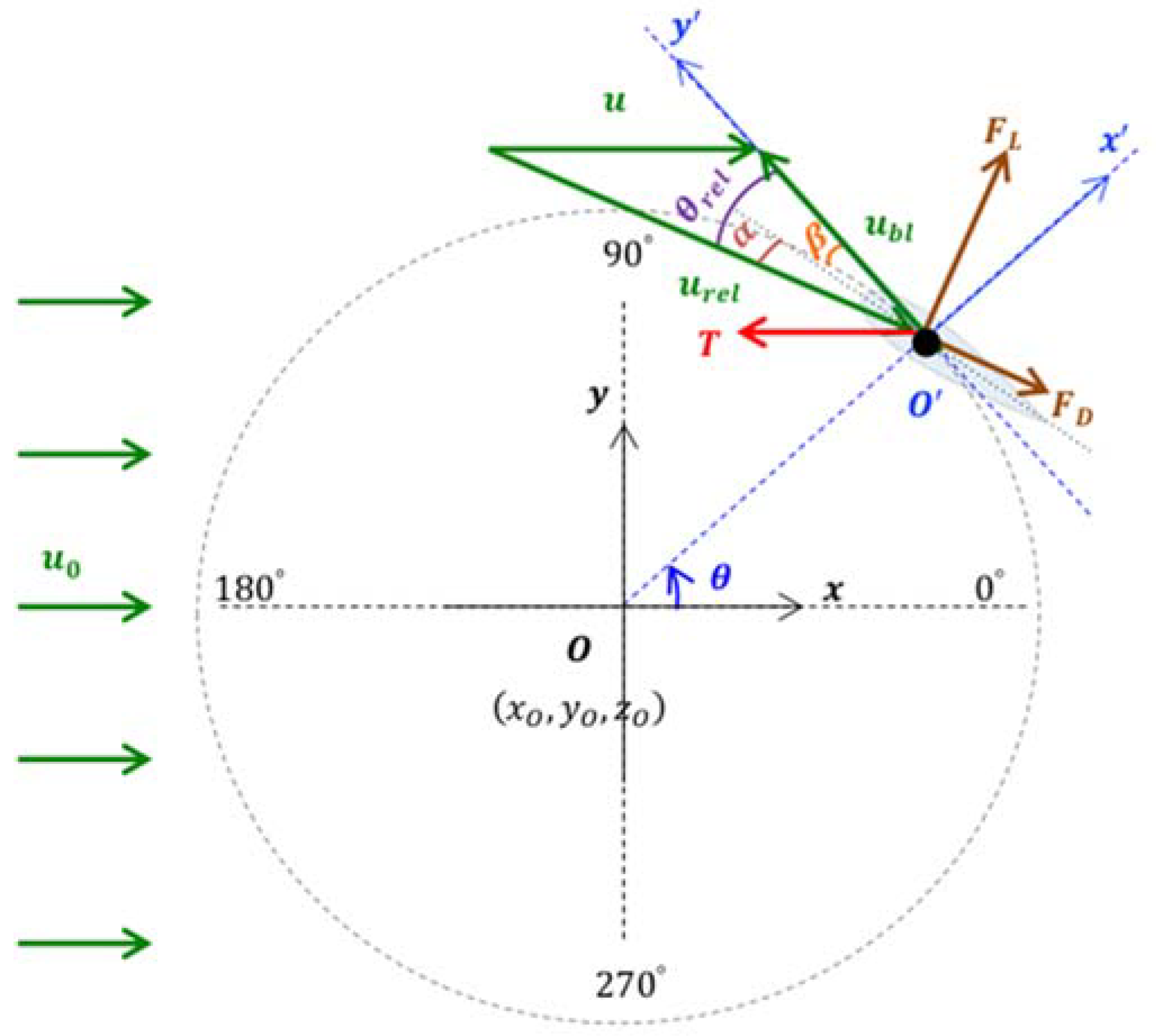
2.1. Frame of Reference
2.2. Lift and Drag Calculations
2.3. Power and Torque Calculation
2.4. Torque Control and Thrust
3. Turbine Parameterization
4. Results and Discussion
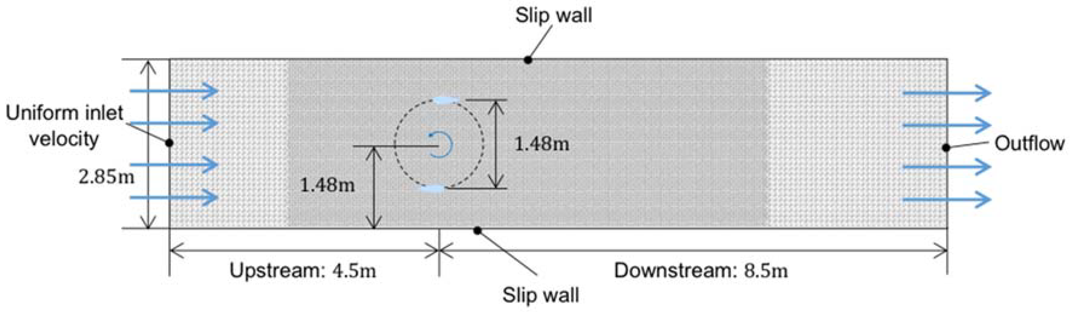
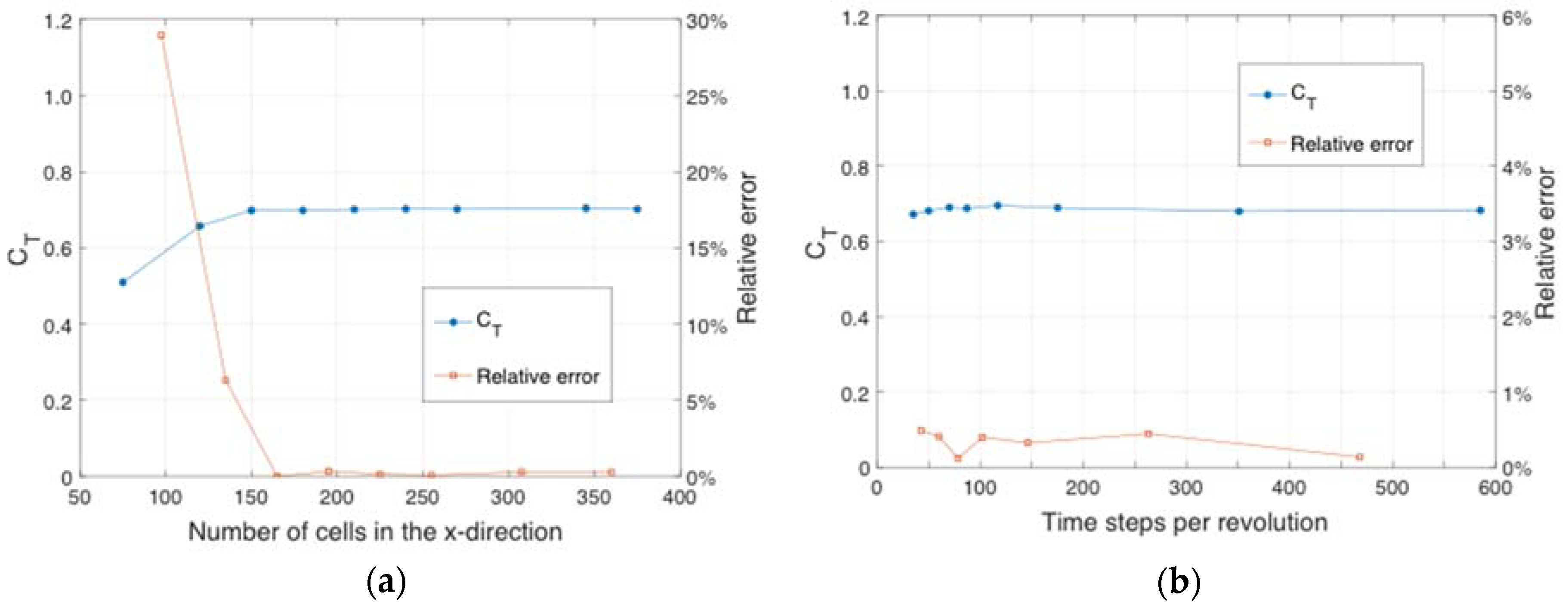
4.1. Validation and Grid Sensitivity Studies
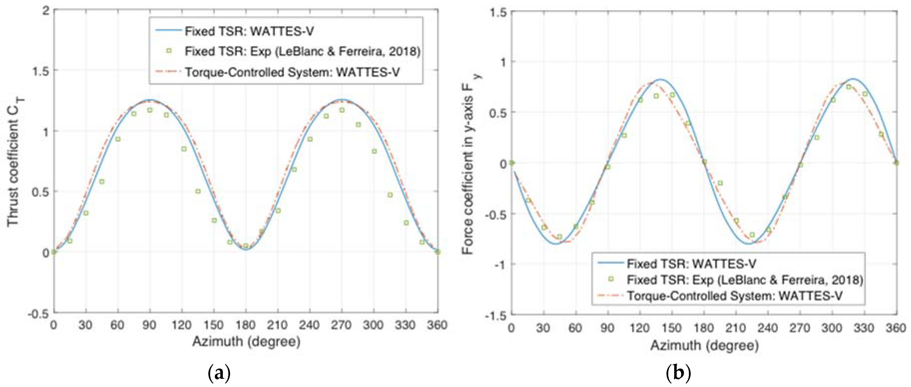
4.2. Two-Bladed H-Type Vertical-Axis Wind Turbine: Fixed Tip Speed Ratio
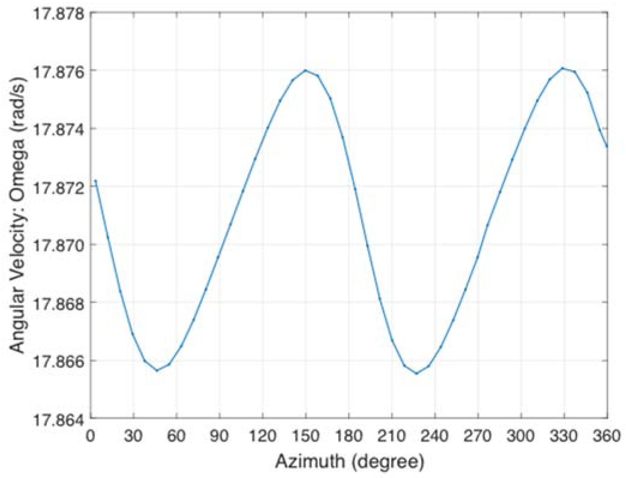
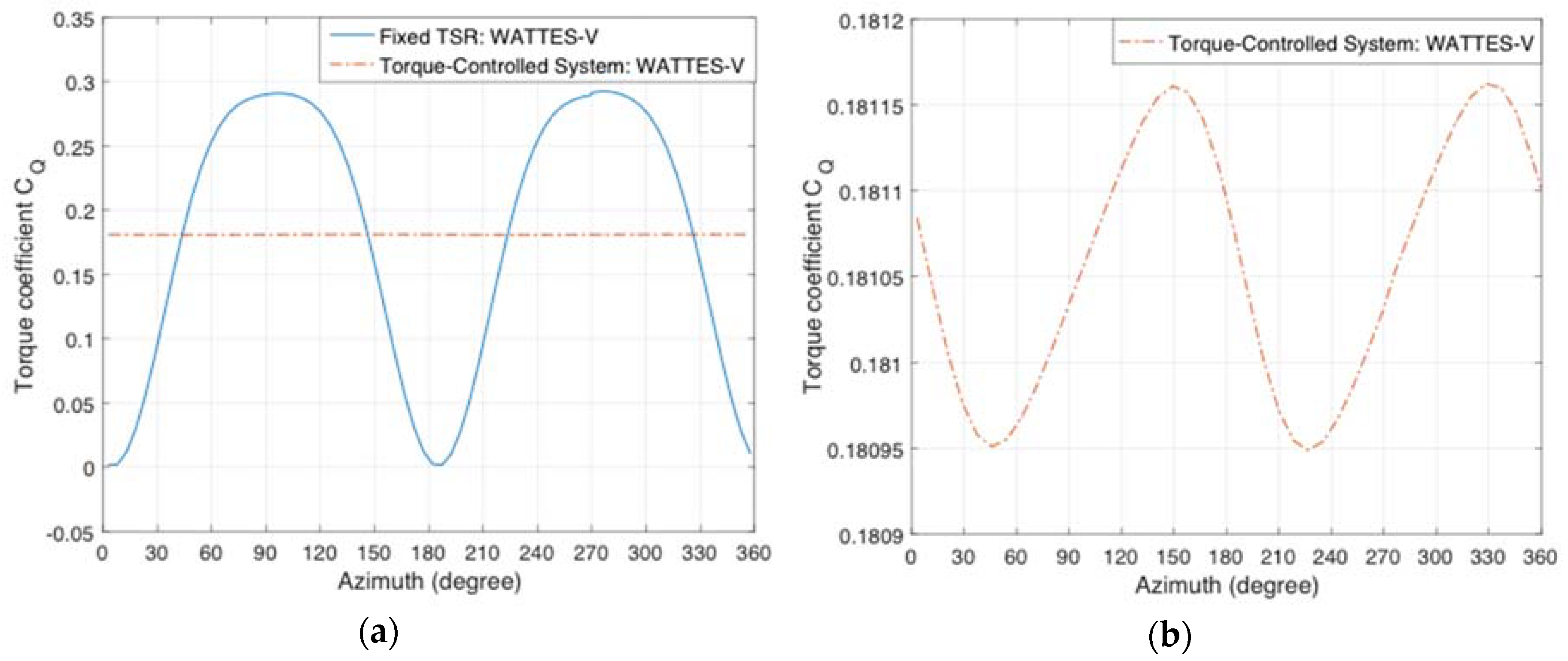
4.3. Two-Bladed H-Type Vertical-Axis Wind Turbine: Torque-Controlled Tip Speed Ratio
5. Conclusions
Author Contributions
Funding
Acknowledgments
Conflicts of Interest
Nomenclature
| Variable | Description |
| Blade chord () | |
| , | Lift and drag coefficients |
| Smallest distance between a given point and the th actuator line () | |
| , | Unit vectors in lift and drag directions |
| , | Drive train efficiency, conversion efficiency |
| , | Lift component per unit span on the th blade () |
| , | Drag component per unit span on the th blade () |
| , | Turbine lift and drag forces per unit span () |
| , | Tangential and normal forces per unit span () |
| , | Body forces per unit span in - and y-axis directions () |
| Moment of inertia () | |
| Blade length () | |
| Blade mass per unit span () | |
| Number of blades | |
| , | Actual power, instantaneous power () |
| Radial distance from the rotor centre () | |
| Reynolds number | |
| Thrust () | |
| Local inflow velocity () | |
| Freestream velocity () | |
| Blade velocity () | |
| Flow relative velocity (m/s) | |
| Azimuthal component of the fluid velocity () | |
| Three components of local velocity () | |
| Coordinates in the original reference frame () | |
| Coordinates in the blade reference frame () | |
| Angle of attack () | |
| Corrected pitch () | |
| Blade pitch () | |
| Local blade twist angle () | |
| Gaussian regularization | |
| Azimuthal angle () | |
| Relative angle () | |
| Fluid density () | |
| Width of the Gaussian kernel | |
| , , | Fluid torque, generator torque, blade torque () |
| Blade angular velocity () | |
| Blade angular acceleration () |
Appendix A
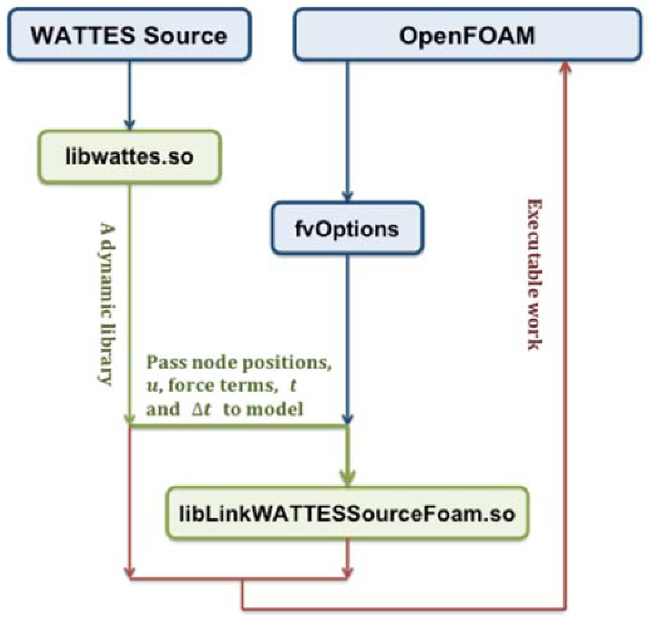
Model Architecture

Appendix B
Appendix B.1. Effect of Mesh Convergence on Near-Wake Vorticity Field

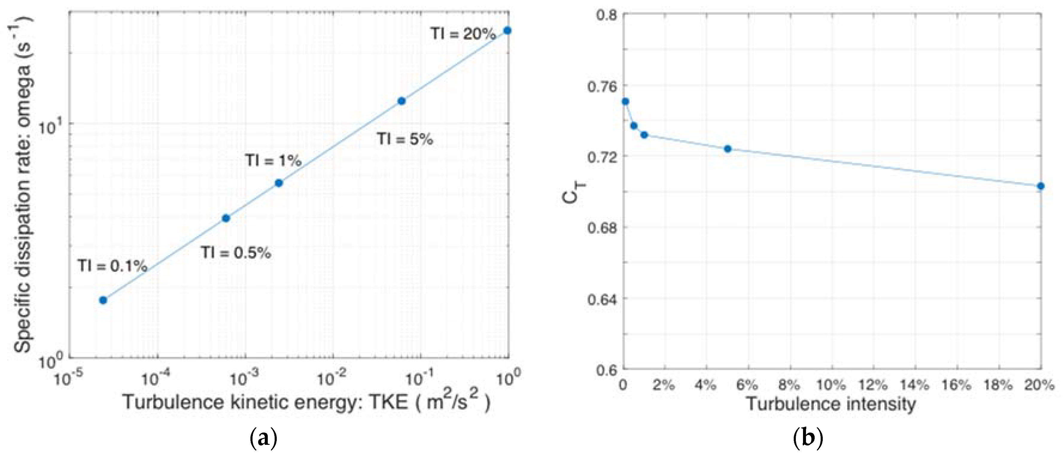
Appendix B.2. Sensitivity Analysis concerning Inlet Turbulence Parameters

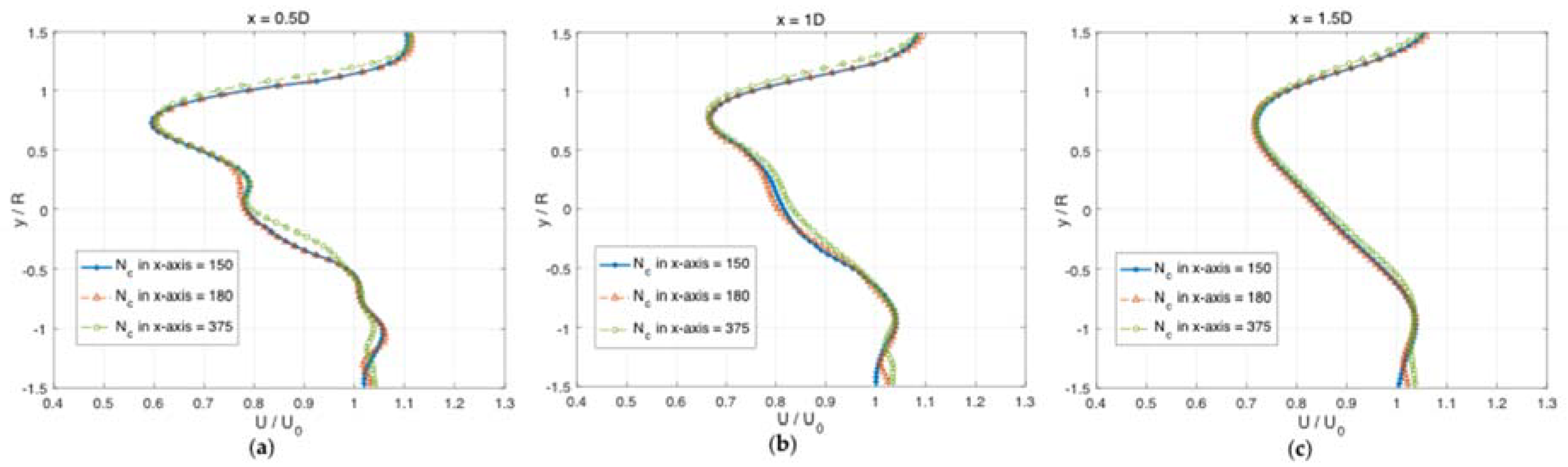
Appendix B.3. Sensitivity Analysis concerning Downstream Domain Size

References
- IEA. Energy and Climate Change; World Energy Outlook Special Report; IEA: Paris, France, 2015; Volume 479, pp. 1–200. [Google Scholar]
- EIA. International Energy Outlook 2017; U.S. Energy Information Administration, Office of Energy Analysis, US Department of Energy: Washington, DC, USA, 2017; p. 20585.
- Borthwick, A.G.L. Marine Renewable Energy Seascape. Engineering 2016, 2, 69–78. [Google Scholar] [CrossRef]
- International Energy Agency. Solutions for the 21st Century; International Energy Agency: Paris, France, 2002. [Google Scholar]
- Wong, K.H.; Chong, W.T.; Sukiman, N.L.; Poh, S.C.; Shiah, Y.-C.; Wang, C.-T. Performance enhancements on vertical axis wind turbines using flow augmentation systems: A review. Renew. Sustain. Rev. 2017, 73, 904–921. [Google Scholar] [CrossRef]
- Salter, S.H. Are nearly all tidal stream turbine designs wrong? In Proceedings of the 4th International Conference on Ocean Energy, Dublin, Ireland, 17–19 October 2012. [Google Scholar]
- Sutherland, H.J.; Berg, D.E.; Ashwill, T.D. A Retrospective of VAWT Technology; Technical Report, Sandia Report, SAND2012-0304; Sandia National Laboratories: Albuquerque, NM, USA, 2012.
- Strom, B.; Johnson, N.; Polagye, B. Impact of blade mounting structures on cross-flow turbine performance. J. Renew. Sustain. Energy 2018, 10, 034504. [Google Scholar] [CrossRef]
- Sahim, K.; Santoso, D.; Puspitasari, D. Investigations on the effect of radius rotor in combined Darrieus-Savonius wind turbine. Int. J. Rotating Mach. 2018, 2018, 3568542. [Google Scholar] [CrossRef]
- Subramanian, A.; Yogesh, S.A.; Sivanandan, H.; Giri, A.; Vasudevan, M.; Mugundhan, V.; Velamati, R.K. Effect of airfoil and solidity on performance of small scale vertical axis wind turbine using three dimensional CFD model. Energy 2017, 133, 179–190. [Google Scholar] [CrossRef]
- Dyachuk, E. Aerodynamics of Vertical-Axis Wind Turbines-Development of Simulation Tools and Experiments. Ph.D. Thesis, Uppsala University, Uppsala, Sweden, 2015. [Google Scholar]
- Salter, S.H.; Taylor, J.R.M. Vertical-axis tidal-current generators and the Pentland Firth. IMechE J. Power Energy 2006, 221, 181–199. [Google Scholar] [CrossRef]
- Suffera, K.H.; Usubamatovb, R.; Quadirc, G.A.; Ismaild, K. Modeling and numerical simulation of a vertical axis wind turbine having cavity vanes. In Proceedings of the 5th International Conference on Intelligent Systems, Modelling and Simulation, Langkawi, Malaysia, 27–29 January 2014. [Google Scholar]
- Dillmann, A.; Heller, G.; Klaas, M.; Kreplin, H.P.; Nitsche, W.; Schröder, W. New Results in Numerical and Experimental Fluid Mechanics VII; Contributions to the 16th STAB/DGLR Symposium Aachen, Germany; Springer: Berlin, Germany, 2008. [Google Scholar]
- Hameed, M.S.; Shahid, F. Evaluation of aerodynamic forces over a vertical axis wind turbine blade through CFD analysis. J. Appl. Mech. Eng. 2012. [Google Scholar] [CrossRef]
- Almohammadi, K.M.; Ingham, D.B.; Ma, L.; Pourkashanian, M. CFD sensitivity analysis of a straight-blade vertical axis wind turbine. Wind Eng. 2012, 36, 571–588. [Google Scholar] [CrossRef]
- Ghatage, S.V.; Joshi, J.B. Optimisation of vertical axis wind turbine: CFD simulations and experimental measurements. Can. J. Chem. Eng. 2012, 90, 1186–1201. [Google Scholar] [CrossRef]
- Zhang, L.X.; Liang, Y.B.; Liu, X.H.; Jiao, Q.F.; Guo, J. Aerodynamic performance prediction of straight-bladed vertical axis wind turbine based on CFD. Adv. Mech. Eng. 2013, 5, 905379. [Google Scholar] [CrossRef]
- Muneer, A.; Khan, M.B.; Sarwar, U.B.; Khan, Z.A.; Badar, M.S. CFD analysis of a Savonius Vertical axis wind turbine. In Proceedings of the 2015 Power Generation Systems and Renewable Energy Technologies, Islamabad, Pakistan, 10–11 June 2015. [Google Scholar]
- Asim, T.; Mishra, R.; Kaysthagir, S.; Aboufares, G. Performance comparison of a vertical axis wind turbine using commercial and open source computational fluid dynamics based codes. In Proceedings of the International Conference on Jets, Wakes and Separated Flows, Stockholm, Sweden, 16–18 June 2015. [Google Scholar]
- Alaimo, A.; Esposito, A.; Messineo, A.; Orlando, C.; Tumino, D. 3D CFD Analysis of a Vertical Axis Wind Turbine. Energies 2015, 8, 3013–3033. [Google Scholar] [CrossRef]
- Bai, C.J.; Lin, Y.Y.; Lin, S.Y.; Wang, W.C. Computational fluid dynamics analysis of the vertical axis wind turbine blade with tubercle leading edge. J. Renew. Sustain. Energy 2015, 7, 033124. [Google Scholar] [CrossRef]
- Rezaeiha, A.; Kalkman, I.; Blocken, B. CFD simulation of a vertical axis wind turbine operating at a moderate tip speed ratio: Guidelines for minimum domain size and azimuthal increment. Renew. Energy 2017, 107, 373–385. [Google Scholar] [CrossRef]
- Unsakul, S.; Sranpat, C.; Chaisiriroj, P.; Leephakpreeda, T. CFD-based performance analysis and experimental investigation of design factors of vertical axis wind turbines under low wind speed conditions in Thailand. J. Flow Control Meas. Vis. 2017, 5, 86–98. [Google Scholar] [CrossRef][Green Version]
- Naccache, G.; Paraschivoiu, M. Development of the dual vertical axis wind turbine using computational fluid dynamics. J. Fluids Eng. 2017, 139, 121105. [Google Scholar] [CrossRef]
- Kao, J.H.; Tseng, P.Y. Application of computational fluid dynamics (CFD) simulation in a vertical axis wind turbine (VAWT) system. IOP Conf. Ser. Earth Environ. 2018, 114, 012002. [Google Scholar] [CrossRef]
- Li, C.; Xiao, Y.; Xu, Y.; Peng, Y.; Hu, G.; Zhu, S. Optimization of blade pitch in H-rotor vertical axis wind turbines through computational fluid dynamics simulations. Appl. Energy 2018, 212, 1107–1125. [Google Scholar] [CrossRef]
- Gokulnath, R.; Devi, P.B.; Senbagan, M.; Manigandan, S. CFD analysis of Savonious type vertical axis wind turbine. IJMET 2018, 9, 1378–1383. [Google Scholar]
- Elsakka, M.M.; Ingham, D.; Ma, L.; Pourkashanian, M. CFD analysis of the angle of attack for a vertical axis wind turbine blade. Energy Convers. Manag. 2019, 182, 154–165. [Google Scholar] [CrossRef]
- Bachant, P.; Goude, A.; Wosnik, M. Actuator line modelling of vertical-axis turbines. arXiv 2018, arXiv:1605.01449v4. [Google Scholar]
- Burton, T.; Jenkins, N.; Sharpe, D.; Bossanyi, E. Wind Energy Handbook, 2nd ed.; Wiley: Hoboken, NJ, USA, 2011. [Google Scholar]
- Okpue, A.S. Aerodynamic Analysis of Vertical and Horizontal Axis Wind Turbines. Master’s Thesis, Michigan State University, East Lansing, MI, USA, 2011. [Google Scholar]
- Shires, A. Development and Evaluation of an Aerodynamic Model for a Novel Vertical Axis Wind Turbine Concept. Energies 2013, 6, 2501–2520. [Google Scholar] [CrossRef]
- Bianchini, A.; Balduzzi, F.; Haack, L.; Bigalli, S.; Müller, B.; Ferrara, G. Development and Validation of a Hybrid Simulation Model for Darrieus Vertical-Axis Wind Turbines. In Proceedings of the ASME Turbo Expo 2019: Turbomachinery Technical Conference and Exposition GT2019-91218, Phoenix, AZ, USA, 17–21 June 2019. [Google Scholar]
- Mikkelsen, R.F. Actuator Disc Methods Applied to Wind Turbines. Ph.D. Thesis, MEK-FM-PHD, No. 2003-02. Technical University of Denmark, Lyngby, Denmark, 2004. [Google Scholar]
- Newman, B.G. Actuator-disc theory for vertical-axis wind turbines. J. Wind Eng. Ind. Aerodyn. 1983, 15, 347–355. [Google Scholar] [CrossRef]
- Linton, D.; Barakos, G.; Widjaja, R.; Thornbern, B. A new actuator surface model with improved wake model for CFD simulations of rotorcraft. In Proceedings of the 73rd Annual Forum and Technology Display of the American Helicopter Society, Fort Worth, TX, USA, 9–11 May 2017. [Google Scholar]
- Shen, W.; Zhang, J.; Sorensen, J. The actuator surface model: A new Navier-Stokes based model for rotor computations. J. Sol. Energy Eng. 2009, 131, 011002. [Google Scholar] [CrossRef]
- Massie, L.; Ouro, P.; Stoesser, T.; Luo, Q. An Actuator Surface Model to Simulate Vertical Axis Turbines. Energies 2019, 12, 4741. [Google Scholar] [CrossRef]
- Bachant, P.; Wosnik, M. Characterising the near-wake of a cross-flow turbine. J. Turbul. 2015, 16, 392–410. [Google Scholar] [CrossRef]
- Riva, L.; Giljarhus, K.E.; Hjertager, B.; Kalvig, S.M. Implementation and application of the actuator line model by OpenFOAM for a vertical axis wind turbine. IOP Conf. Ser. Mater. Sci. Eng. 2017, 276, 012002. [Google Scholar] [CrossRef]
- Sørensen, J.N.; Shen, W.Z. Numerical modelling of wind turbine wakes. J. Fluids Eng. 2002, 124, 393–399. [Google Scholar] [CrossRef]
- Troldborg, N. Actuator Line Modelling of Wind Turbine Wakes. Ph.D. Thesis, Technical University of Denmark, Lyngby, Denmark, June 2008. [Google Scholar]
- Martinez, L.; Leonardi, S.; Churchfield, M.; Moriarty, P. A comparison of actuator disk and actuator line wind turbine models and best practices for their use. AIAA J. 2012, 16. [Google Scholar] [CrossRef]
- Shamsoddin, S.; Porté-Agel, F. Large Eddy Simulation of vertical axis wind turbine wakes. Energies 2014, 7, 890–912. [Google Scholar] [CrossRef]
- Reynolds, O. On the dynamical theory of incompressible viscous fluids and the determination of the criterion. Philos. Trans. R. Soc. Lond. A 1895, 186, 123–164. [Google Scholar]
- Hanjalic, K.; Launder, B. A Reynolds stress model of turbulence and its application to thin shear flows. J. Fluid Mech. 1972, 52, 609–638. [Google Scholar] [CrossRef]
- Wilcox, D.C. Turbulence Modelling for CFD, 2nd ed.; DCW Industries Inc.: La Canada, CA, USA, 1998. [Google Scholar]
- Wilcox, D.C. Formulation of the k-omega Turbulence Model Revisited. AIAA J. 2008, 46, 11. [Google Scholar] [CrossRef]
- Deardorff, J. A numerical study of three-dimensional turbulent channel flow at large Reynolds numbers. J. Fluid Mech. 1970, 41, 453–480. [Google Scholar] [CrossRef]
- Smagorinsky, J. General Circulation Experiments with the Primitive Equation. Mon. Weather Rev. 1963, 91, 99. [Google Scholar] [CrossRef]
- Creech, A.C.W. A Three-Dimensional Numerical Model of a Horizontal Axis, Energy Extracting Turbine. Ph.D. Thesis, Heriot-Watt University, Edinburgh, Scotland, UK, March 2009. [Google Scholar]
- Creech, A.; Früh, W.-G.; Clive, P. Actuator volumes and hr-adaptive methods for three-dimensional simulation of wind turbine wakes and performance. Wind Energy 2011, 15, 847–863. [Google Scholar] [CrossRef]
- Creech, A.C.W.; Früh, W.G.; Maguire, A.E. Simulations of an offshore wind farm using large eddy simulation and a torque-controlled actuator disc model. Surv. Geophys. 2015, 36, 427–481. [Google Scholar] [CrossRef]
- Creech, A.; Früh, W.-G. Modelling wind turbine wakes for wind farms. In Alternative Energy and Shale Gas Encyclopedia; Lehr, J., Keeley, J., Eds.; The University of Edinburgh: Edinburgh, UK, 2016. [Google Scholar]
- Creech, A.C.W.; Borthwick, A.G.L.; Ingram, D. Effects of support structures in an LES actuator line model of a tidal turbine with contra-rotating rotors. Energies 2017, 10, 726. [Google Scholar] [CrossRef]
- McLaren, K.W. Unsteady Loading of High Solidity Vertical Axis Wind Turbines. Ph.D. Thesis, McMaster University, Hamilton, ON, Canada, 2011. [Google Scholar]
- Nobile, R.; Vahdati, M.; Barlow, J.F. Unsteady flow simulation of a vertical axis wind turbine: A two-dimensional study. J. Wind Eng. Ind. Aerodyn. 2014, 125, 168–179. [Google Scholar] [CrossRef]
- Biadgo, A.M.; Simonovic, A.; Komarov, D.; Stupar, S. Numerical and analytical investigation of vertical axis wind turbine. FME Trans. 2013, 41, 49–58. [Google Scholar]
- Bachant, P.; Wosnik, M. Modelling the near-wake of a vertical-axis cross-flow turbine with 2-D and 3-D RANS. J. Renew. Sustain. Energy 2016, 8, 053311. [Google Scholar] [CrossRef]
- Krogstad, P.A.; Eriksen, P.E. Blind test calculations of the performance and wake development for a model wind turbine. Renew. Energy 2013, 50, 325–333. [Google Scholar] [CrossRef]
- Buntine, J.D.; Pullin, D.I. Merger and cancellation of strained vortices. J. Fluid Mech. 1989, 205, 263–295. [Google Scholar] [CrossRef]
- Rezaeiha, A.; Kalkman, I.; Blocken, B. Effect of pitch angle on power performance and aerodynamics of a vertical axis wind turbine. Appl. Energy 2017, 197, 132–150. [Google Scholar] [CrossRef]
- Hwang, I.S.; Lee, Y.H.; Kim, S.J. Optimization of cycloidal water turbine and the performance improvement by individual blade control. Appl. Energy 2009, 86, 1532–1540. [Google Scholar] [CrossRef]
- Zhao, R.; Creech, A.C.W.; Borthwick, A.G.L.; Nishino, T. Coupling of WATTES and OpenFOAM codes for wake modelling behind close-packed contra-rotating vertical-axis tidal rotors. In Proceedings of the 6th Oxford Tidal Energy Workshop, Oxford, UK, 26–27 March 2018. [Google Scholar]
- Schito, P.; Zasso, A. Actuator forces in CFD: RANS and les modelling in OpenFOAM. J. Phys. Conf. Ser. 2014, 524, 012160. [Google Scholar] [CrossRef]
- Jha, P.K.; Churchfield, M.J.; Moriarty, P.J.; Schmitz, S. Guidelines for volume force distributions within actuator line modelling of wind turbines on large-eddy simulation-type grids. J. Sol. Energy Eng. 2014, 136, 031003. [Google Scholar] [CrossRef]
- Martínez-Tossas, L.A.; Churchfield, M.J.; Meneveau, C. Optimal smoothing length scale for actuator line models of wind turbine blades. Wind Energy 2015, 20, 1083–1096. [Google Scholar] [CrossRef]
- Tennekes, H.; Lumley, J.L. A First Course in Turbulence; The MIT Press: Cambridge, MA, USA, 1972. [Google Scholar]
- LeBlanc, B.P.; Ferreira, C.S. Experimental determination of thrust loading of a 2-bladed vertical axis wind turbine. J. Phys. Conf. Ser. 2018, 1037, 022043. [Google Scholar] [CrossRef]
- Menter, F.R. Two-Equation Eddy-Viscosity Turbulence Models for Engineering Applications. AIAA J. 1994, 32, 8. [Google Scholar] [CrossRef]
- Barthelmie, R.J.; Hansen, K.; Frandsen, S.T.; Rathmann, O.; Schepers, J.G.; Schlez, W.; Phillips, J.; Rados, K.; Zervos, A.; Politis, E.S.; et al. Modelling and measuring flow and wind turbine wakes in large wind farms offshore. Wind Energy 2009, 12, 431–444. [Google Scholar] [CrossRef]
- Bachant, P. Physical and numerical modeling of cross-flow turbines. Ph.D. Thesis, University of New Hampshire, Durham, NC, USA, 2016. [Google Scholar]
- Roache, P.J. Perspective: A method for uniform reporting of grid refinement studies. J Fluid Eng. ASME 1994, 116, 405–413. [Google Scholar] [CrossRef]
- Bakhvalov, N.S. Courant–Friedrichs–Lewy condition. In Encyclopedia of Mathematics; Michiel, H., Ed.; Springer Science + Business Media, B.V./Kluwer Academic Publishers: Berlin, Germany, 2001; ISBN 978-1-55608-010-4. [Google Scholar]
- Sheldahl, R.E.; Klimas, P.C. Aerodynamic Characteristics of Seven Symmetrical Airfoil Sections through 180-Degree Angle of Attack for Use in Aerodynamic Analysis of Vertical Axis Wind Turbines; Energy Report; Sandia National Lab: Albuquerque, NM, USA, 1981.
- Ouro, P.; Stoesser, T. An immersed boundary-based large-eddy simulation approach to predict the performance of vertical axis tidal turbines. Comput. Fluids 2017, 152, 74–87. [Google Scholar] [CrossRef]
- Brochier, G.; Fraunie, P.; Beguier, C.; Paraschivoiu, I. Water channel experiments of dynamic stall on Darrieus wind turbine blades. J. Propuls. Power 1986, 2, 445–449. [Google Scholar] [CrossRef]
- Araya, D.B.; Dabiri, J.O. A comparison of wake measurements in motor-driven and flow-driven turbine experiments. Exp. Fluids 2015, 56, 150. [Google Scholar] [CrossRef]
- Ouro, P.; Runge, S.; Luo, Q.; Stoesser, T. Three-dimensionality of the wake recovery behind a vertical axis turbine. Renew. Energy 2018, 133, 1066–1077. [Google Scholar] [CrossRef]
- Piggott, M.; Pain, C.; Gorman, G.; Power, P.; Goddard, A. h, r, and hr adaptivity with applications in numerical ocean modelling. Ocean Model 2004, 10, 95–113. [Google Scholar] [CrossRef]
- Jensen, B.B.B. Numerical study of influence of inlet turbulence parameters on turbulence intensity in the flow domain: Incompressible flow in pipe system. Proc. IMechE Part E J. Process Mech. Eng. 2007, 221, 177–185. [Google Scholar] [CrossRef]
- User Guide: K-Omega Shear Stress Transport (SST)—OpenFOAM. Available online: https://www.openfoam.com/documentation/guides/latest/doc/guide-turbulence-ras-k-omega-sst.html (accessed on 2 February 2020).


| Property | Symbol | Value/Dimension |
|---|---|---|
| Number of blades | ||
| Turbine diameter | ||
| Blade length | ||
| Aerofoil type | ||
| Chord | ||
| Blade pitch | ||
| Freestream flow speed | ||
| Fluid density | ||
| Local Reynolds number |
© 2020 by the authors. Licensee MDPI, Basel, Switzerland. This article is an open access article distributed under the terms and conditions of the Creative Commons Attribution (CC BY) license (http://creativecommons.org/licenses/by/4.0/).
Share and Cite
Zhao, R.; Creech, A.C.W.; Borthwick, A.G.L.; Venugopal, V.; Nishino, T. Aerodynamic Analysis of a Two-Bladed Vertical-Axis Wind Turbine Using a Coupled Unsteady RANS and Actuator Line Model. Energies 2020, 13, 776. https://doi.org/10.3390/en13040776
Zhao R, Creech ACW, Borthwick AGL, Venugopal V, Nishino T. Aerodynamic Analysis of a Two-Bladed Vertical-Axis Wind Turbine Using a Coupled Unsteady RANS and Actuator Line Model. Energies. 2020; 13(4):776. https://doi.org/10.3390/en13040776
Chicago/Turabian StyleZhao, Ruiwen, Angus C. W. Creech, Alistair G. L. Borthwick, Vengatesan Venugopal, and Takafumi Nishino. 2020. "Aerodynamic Analysis of a Two-Bladed Vertical-Axis Wind Turbine Using a Coupled Unsteady RANS and Actuator Line Model" Energies 13, no. 4: 776. https://doi.org/10.3390/en13040776
APA StyleZhao, R., Creech, A. C. W., Borthwick, A. G. L., Venugopal, V., & Nishino, T. (2020). Aerodynamic Analysis of a Two-Bladed Vertical-Axis Wind Turbine Using a Coupled Unsteady RANS and Actuator Line Model. Energies, 13(4), 776. https://doi.org/10.3390/en13040776