Optimal Placement, Sizing and Coordination of FACTS Devices in Transmission Network Using Whale Optimization Algorithm

 , ,
, ,
Abstract
1. Introduction
1.1. Stability Issues of Power Transmission
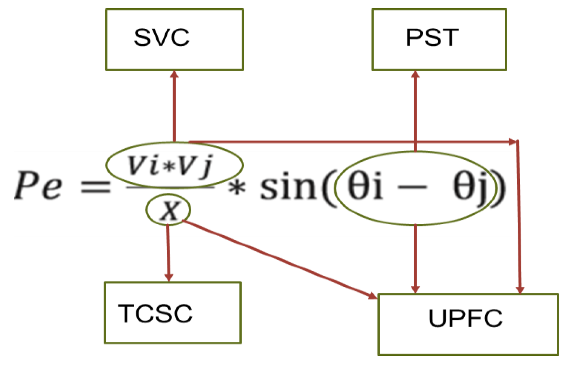
1.2. Controlled Parameters of Different FACTS
2. Modeling of FACTS
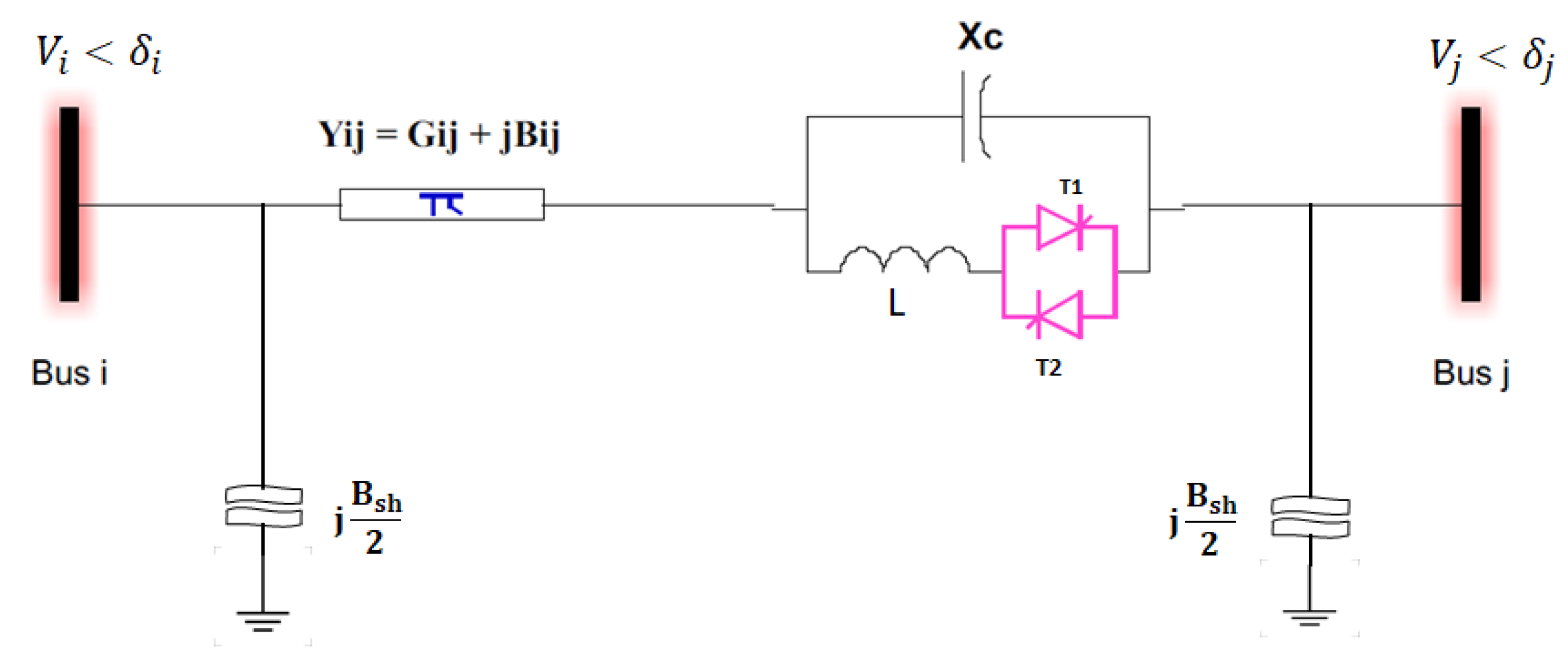
2.1. Modeling of TCSC
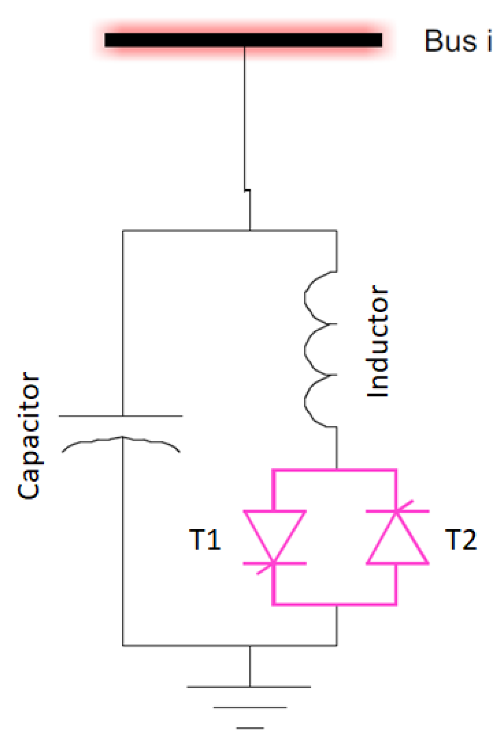
2.2. Modeling of SVC
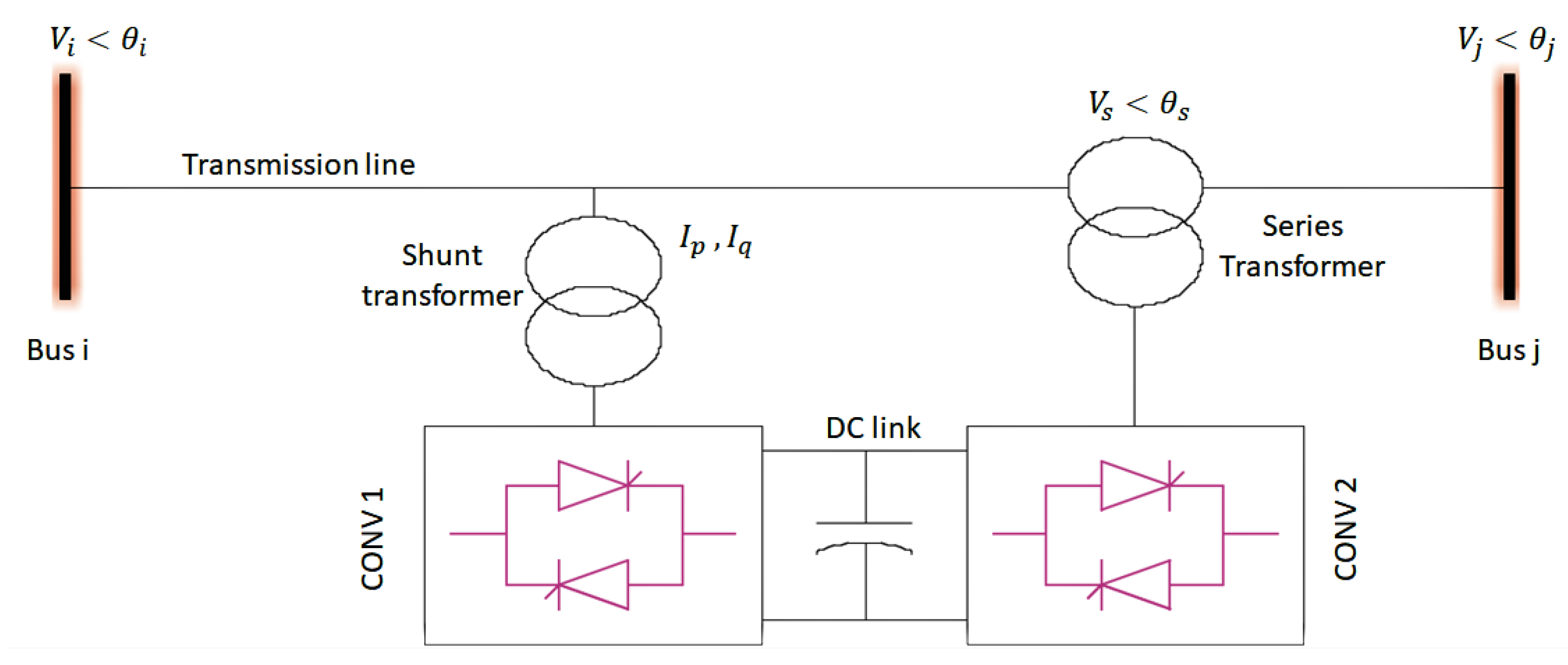
2.3. Modeling of UPFC
3. Optimal Placement of FACTS
3.1. Optimal Placement of TCSC
3.2. Optimal Placement of SVC
3.3. Optimal Placement of UPFC
4. Problem Formulation
- Bus voltages should be in their appropriate limits as
- Thermal limits of transmission lineswhere is the apparent power flowing through the line in Mega Volt Ampere (MVA).
- Generator’s reactive power supply limits
- Limit on the arrangements of the transformer tap setting
- SVC size constraintswhere ZSVC is the size of the SVC in pu.
- TCSC size constraintswhere XTCSC is the size of the TCSC in pu
5. Whale Optimization Algorithm
- Encircling prey
- Exploitation phase
- Exploration phase
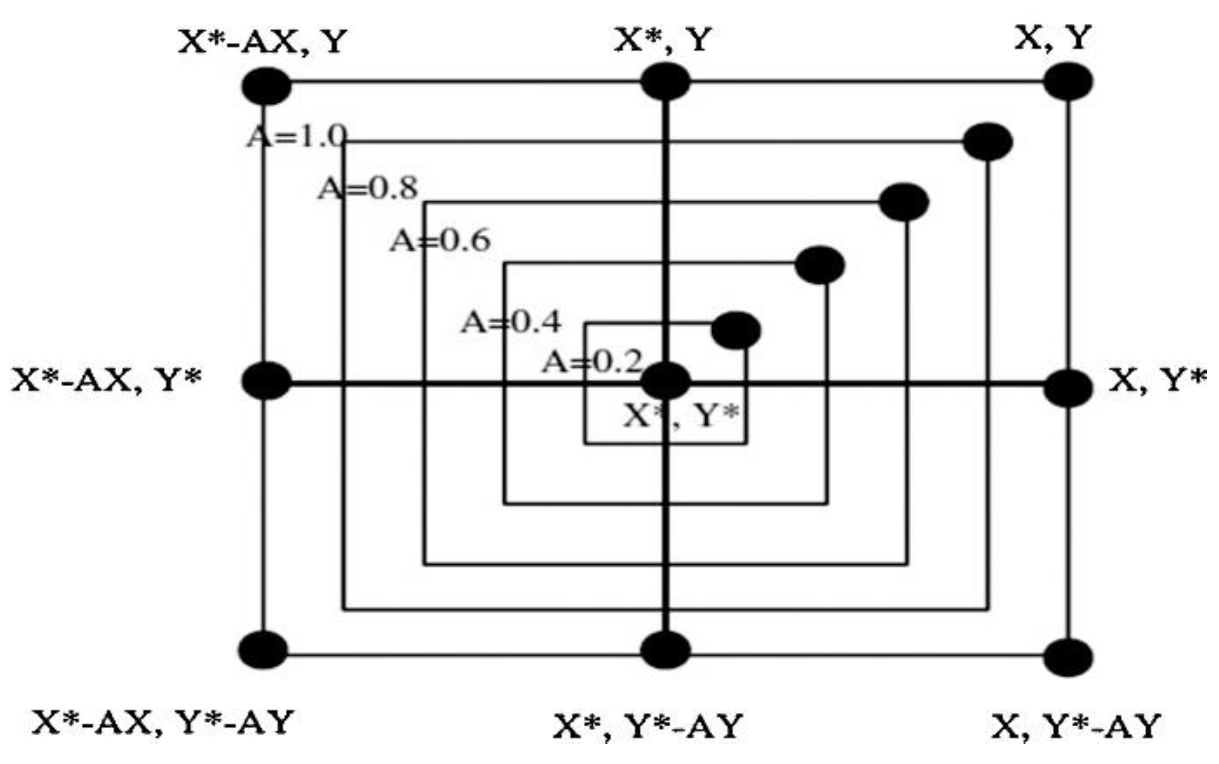
5.1. Encircling Prey
5.2. Exploitation Phase
5.2.1. Shrinking-Encircling Technique
5.2.2. Spirals-Updating Position Technique
5.3. Searching for Prey (Exploration-Phase)
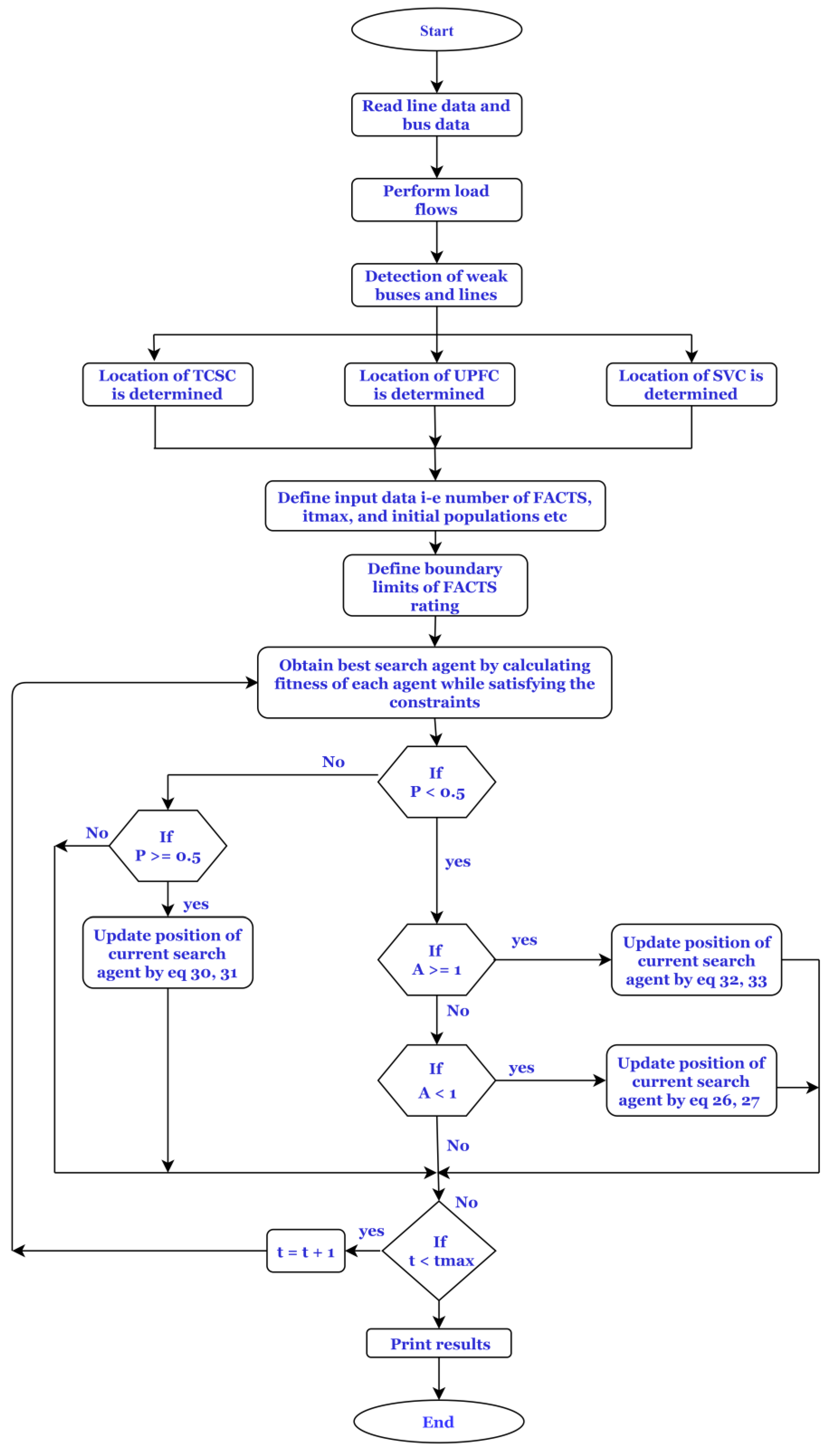
5.4. Flowchart

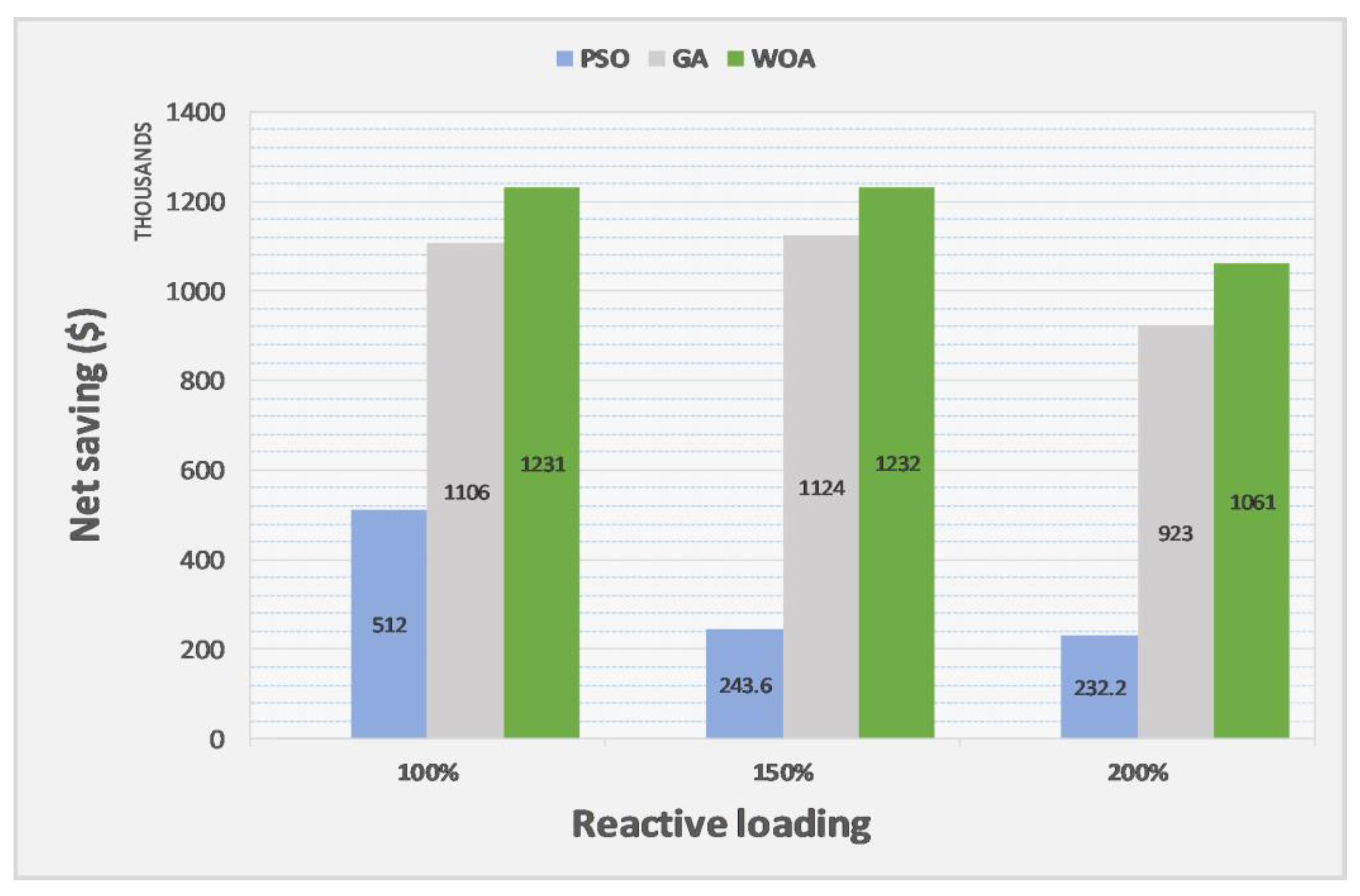
6. Results and Discussions
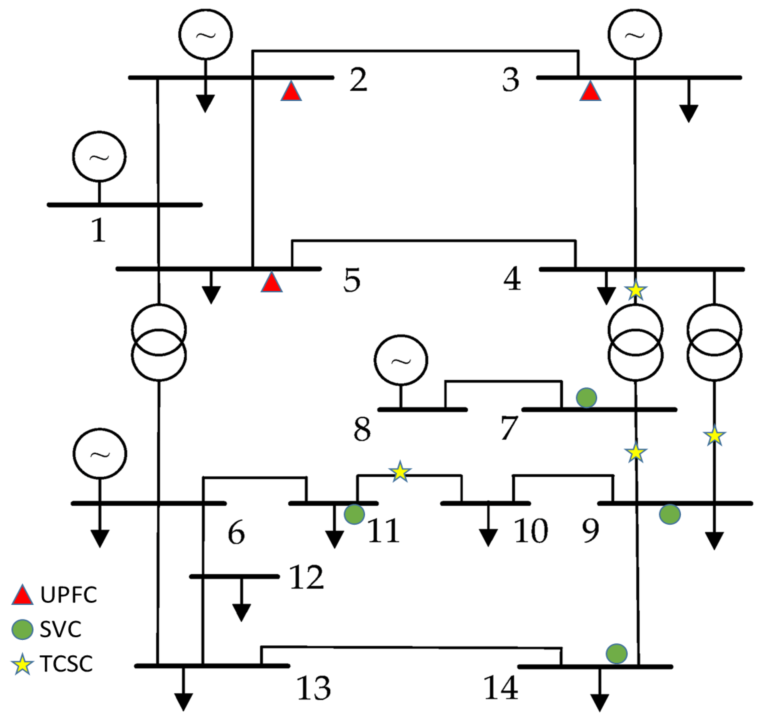
6.1. Test Case IEEE-14 Bus System
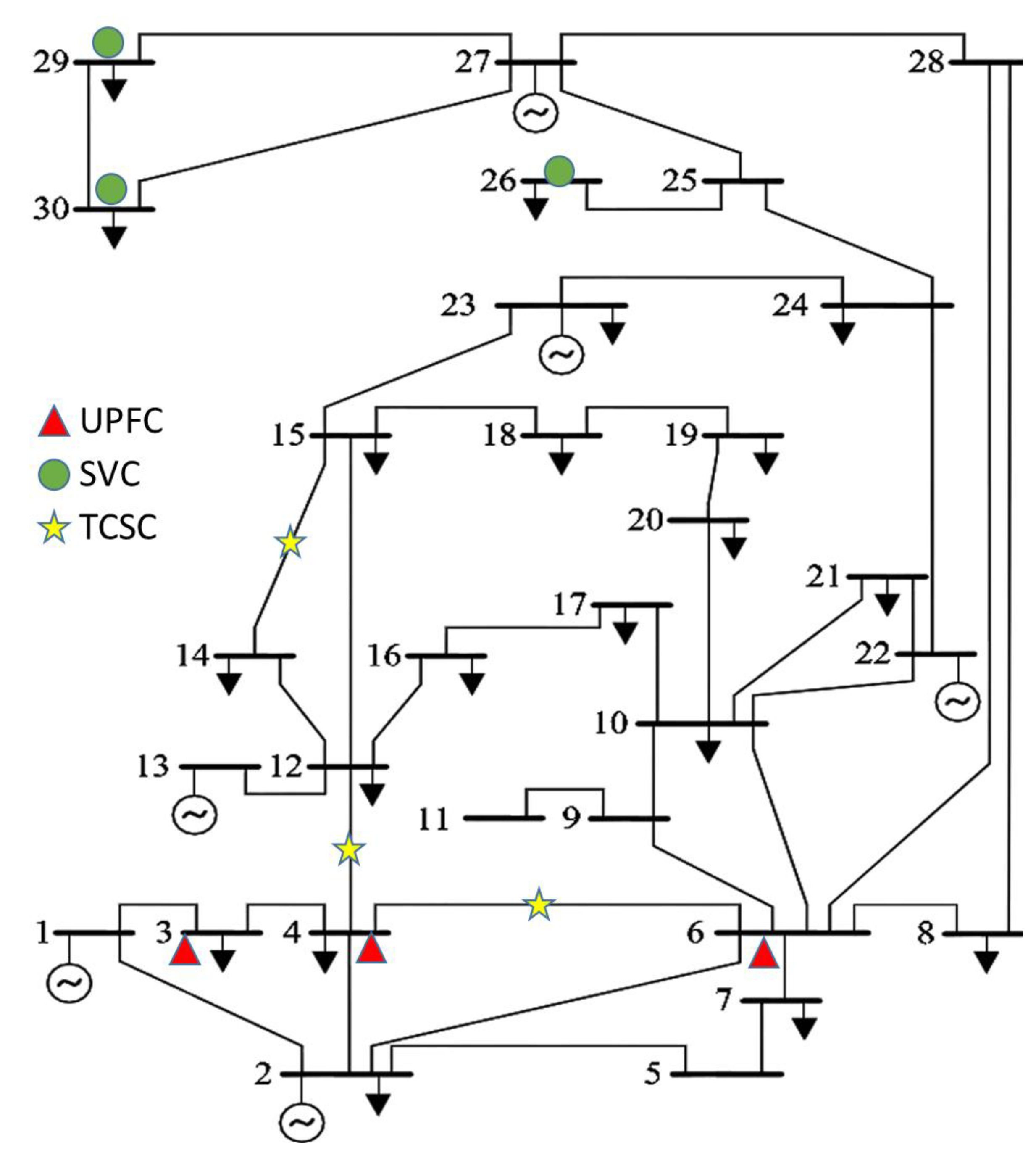
6.2. Test Case IEEE 30 Bus System
7. Conclusions
Author Contributions
Funding
Acknowledgments
Conflicts of Interest
References
- Liu, S.; Cruzat, C.; Kopsidas, K. Impact of transmission line overloads on network reliability and conductor ageing. In Proceedings of the 2017 IEEE, Manchester, UK, 18–22 June 2017; pp. 1–5. [Google Scholar]
- Prabha, K. Power System Stability and Control, 1st ed.; Neal, J., Baja, M.G.L., Eds.; McGraw-Hill, Inc.: New York, NY, USA, 1994. [Google Scholar]
- Aboreshaid, S.; Billinton, R. Probabilistic evaluation of voltage stability. IEEE Trans. Power Syst. 1999, 14, 342–348. [Google Scholar] [CrossRef]
- Ghahremani, E.; Kamwa, I. Optimal Placement of Multiple-Type FACTS Devices to Maximize Power System Loadability Using a Generic Graphical User Interface. IEEE Trans. Power Syst. 2012, 1–15. [Google Scholar] [CrossRef]
- Chansareewittaya, S.; Jirapong, P. Power transfer capability enhancement with optimal maximum number of facts controllers using evolutionary programming. In Proceedings of the IECON 2011—37th Annual Conference of the IEEE Industrial Electronics Society, Melbourne, VIC, Australia, 7–10 November 2011; pp. 4733–4738. [Google Scholar]
- Tlijani, K.; Guesmi, T.; Hadj Abdallah, H. Optimal number, location and parameter setting of multiple TCSCs for security and system loadability enhancement. In Proceedings of the 10th International Multi-Conferences on Systems, Signals & Devices 2013 (SSD13), Hammamet, Tunisia, 18–21 March 2013; pp. 1–6. [Google Scholar]
- Sode-yome, A.; Mithulananthan, N.; Lee, K.Y. Reactive Power Loss Sensitivity Approach in Placing FACTS Devices and UPFC; IFAC: New York, NY, USA, 2004; Volume 45. [Google Scholar]
- Faried, S.O.; Billinton, R.; Aboreshaid, S. Probabilistic technique for sizing FACTS devices for steady-state voltage profile enhancement. IET Gener. Transm. Distrib. 2009, 3, 385–392. [Google Scholar] [CrossRef]
- Nascimento, S.D.; Gouvêa, M.M. Voltage Stability Enhancement in Power Systems with Automatic Facts Device Allocation. Energy Procedia 2017, 107, 60–67. [Google Scholar] [CrossRef]
- Barrios-Martínez, E.; Ángeles-Camacho, C. Technical comparison of FACTS controllers in parallel connection. J. Appl. Res. Technol. 2017, 15, 36–44. [Google Scholar] [CrossRef]
- Cai, L.J.; Erlich, I.; Stamtsis, G.C. Optimal choice and allocation of FACTS devices in deregulated electricity market using genetic algorithms. In Proceedings of the IEEE PES Power Systems Conference and Exposition, New York, NY, USA, 10–13 October 2004; pp. 201–207. [Google Scholar]
- Zahid, M.; Chen, J.; Li, Y. Application of AAA for Optimized Placement of UPFC in Power systems. In Proceedings of the 2018 13th IEEE Conference on Industrial Electronics and Applications (ICIEA), Wuhan, China, 31 May–2 June 2018; pp. 30–35. [Google Scholar]
- Alharbi, F.T.; Almasabi, S.; Mitra, J. Enhancing Network Loadability Using Optimal TCSC Placement and Sizing. In Proceedings of the 2018 IEEE/PES Transmission and Distribution Conference and Exposition (T&D), Denver, CO, USA, 16–19 April 2018; pp. 1–9. [Google Scholar]
- Dawn, S.; Kumar Tiwari, P.; Kumar Goswami, A.; Panda, R. An approach for system risk assessment and mitigation by optimal operation of wind farm and FACTS devices in a centralized competitive power market. IEEE Trans. Sustain. Energy 2019, 10, 1054–1065. [Google Scholar] [CrossRef]
- Dawn, S.; Tiwari, P.K.; Goswami, A.K. An approach for long term economic operations of competitive power market by optimal combined scheduling of wind turbines and FACTS controllers. Energy 2019, 181, 709–723. [Google Scholar] [CrossRef]
- Hermanu, C.; Nizam, M.; Robbani, F.I. Optimal Placement of Unified Power Flow Controllers (UPFC) for Losses Reduction and Improve Voltage Stability Based on Sensitivity Analysis in 500 kV Java-Bali Electrical Power System. In Proceedings of the 2018 5th International Conference on Electric Vehicular Technology (ICEVT), Surakarta, Indonesia, 30–31 Octber 2018; pp. 83–87. [Google Scholar]
- Jamnani, J.G.; Pandya, M. Coordination of SVC and TCSC for management of power flow by particle swarm optimization. Energy Procedia 2019, 156, 321–326. [Google Scholar] [CrossRef]
- Magadum, R.B.; Dodamani, S.N.; Kulkarni, D.B. Optimal Placement of Unified Power Flow Controller (UPFC) using Fuzzy Logic. In Proceedings of the 2019 Fifth International Conference on Electrical Energy Systems (ICEES), Chennai, India, 21–22 February 2019; pp. 1–4. [Google Scholar]
- Ziaee, O.; Choobineh, F.F. Thyristor-controlled switch capacitor placement in large-scale power systems via mixed integer linear programming and Taylor series expansion. In Proceedings of the 2014 IEEE PES General Meeting|Conference & Exposition, National Harbor, MD, USA, 27–31 July 2014; p. 777. [Google Scholar]
- Bhattacharyya, B.; Kumar, S. Approach for the solution of transmission congestion with multi-type FACTS devices. IET Gener. Transm. Distrib. 2016, 10, 2802–2809. [Google Scholar] [CrossRef]
- Galvani, S.; Banna Sharifian, M.B.; Tarafdar Hagh, M. Unified power flow controller impact on power system predictability. IET Gener. Transm. Distrib. 2014, 8, 819–827. [Google Scholar] [CrossRef]
- Inkollu, S.R.; Kota, V.R. Optimal setting of FACTS devices for voltage stability improvement using PSO adaptive GSA hybrid algorithm. Eng. Sci. Technol. Int. J. 2016, 19, 1166–1176. [Google Scholar] [CrossRef]
- Mohammadi, A.; Jazaeri, M. A hybrid particle swarm optimization-genetic algorithm for optimal location of SVC devices in power system planning. In Proceedings of the 42nd International Universities Power Engineering Conference, Brighton, UK, 4–6 September 2007; pp. 1175–1181. [Google Scholar]
- Kulkarni, P.P. Optimal Placement and Parameter setting of TCSC in Power Transmission System to increase the Power Transfer Capability. In Proceedings of the 2015 International Conference on Energy Systems and Applications (ICESA), Pune, India, 30 October–1 November 2015; pp. 735–739. [Google Scholar]
- Khan, I.; Mallick, M.A.; Rafi, M.; Mirza, M.S. Optimal placement of FACTS controller scheme for enhancement of power system security in Indian scenario. J. Electr. Syst. Inf. Technol. 2015, 2, 161–171. [Google Scholar] [CrossRef]
- Kavitha, K.; Neela, R. Optimal allocation of multi-type FACTS devices and its effect in enhancing system security using BBO, WIPSO & PSO. J. Electr. Syst. Inf. Technol. 2017, 1–17. [Google Scholar]
- Bhattacharyya, B.; Kumar, S. Electrical Power and Energy Systems Loadability enhancement with FACTS devices using gravitational search algorithm. Int. J. Electr. Power Energy Syst. 2016, 78, 470–479. [Google Scholar] [CrossRef]
- Preedavichit, P.; Srivastava, S.C. Optimal reactive power dispatch considering FACTS devices. In Proceedings of the 1997 Fourth International Conference on Advances in Power System Control, Operation and Management, APSCOM-97 (Conf. Publ. No. 450), Hong Kong, China, 11–14 November 1997; pp. 620–625. [Google Scholar]
- Raj, S.; Bhattacharyya, B. Optimal placement of TCSC and SVC for reactive power planning using Whale optimization algorithm. Swarm Evol. Comput. 2018, 40, 131–143. [Google Scholar] [CrossRef]
- Bansal, H.O.; Agrawal, H.P.; Tiwana, S.; Singal, A.R.; Shrivastava, L. Optimal Location of FACT Devices to Control Reactive Power. Int. J. Eng. Sci. Technol. 2010, 2, 1556–1560. [Google Scholar]
- Padhy, N.P.; Abdel-Rahim, A.M.M. Optimal Placement of Facts Devices for Practical Utilities. Int. J. Power Energy Syst. 2007, 27, 1–31. [Google Scholar] [CrossRef]
- Narain, G.H. Understanding FACTs Concepts and Tehnology of Flexible AC Transmission Systems; Wiley-IEEE Press: New York, NY, USA, 2000; Volume 136. [Google Scholar]
- Gyugyi, L. Unified power-flow control concept for flexible AC transmission systems. Gener. Transm. Distrib. IEE Proc. C 1992, 139, 323–331. [Google Scholar] [CrossRef]
- Masood, T.; Shah, S.K.; Tajammal, M.; Qureshi, S.A.; Khan, A.J.; Jameel, N.; Kothari, D.P. Unified power flow controller modeling and analysis technique on the GCC power grid. In Proceedings of the 2018 IEEE International Energy Conference (ENERGYCON), Limassol, Cyprus, 3–7 June 2018; pp. 1–6. [Google Scholar]
- Bhattacharyya, B.; Gupta, V.K.; Kumar, S. UPFC with series and shunt FACTS controllers for the economic operation of a power system. Ain Shams Eng. J. 2014, 5, 775–787. [Google Scholar] [CrossRef]
- Musirin, I.; Abdul Rahman, T.K. Novel fast voltage stability index (FVSI) for voltage stability analysis in power transmission system. In Proceedings of the Student Conference on Research and Development, Shah Alam, Malaysia, 17 July 2002; pp. 265–268. [Google Scholar]
- Moghavvemi, M.; Faruque, O. Real-time contingency evaluation and ranking technique. IEE Proc.—Gener. Transm. Distrib. 2002, 145, 517. [Google Scholar] [CrossRef]
- Moghavvemi, M.; Omar, F.M. Technique for contingency monitoring and voltage collapse prediction. IEE Proc.—Gener. Transm. Distrib. 1998, 145, 634. [Google Scholar] [CrossRef]
- Ajjarapu, V.; Christy, C. The continuation power flow: A tool for steady state voltage stability analysis. IEEE Trans. Power Syst. 1992, 7, 416–423. [Google Scholar] [CrossRef]
- Milano, F. An open source power system analysis toolbox. IEEE Trans. Power Syst. 2005, 20, 1199–1206. [Google Scholar] [CrossRef]
- Cai, L.J.; Erlich, I. Optimal Choice and Allocation of FACTS Devices using Genetic Algorithms. Optim. Choice Alloc. FACTS Devices Using Genet. Algorithms 2004, 2004, 1–6. [Google Scholar]
- Mirjalili, S.; Lewis, A. The Whale Optimization Algorithm. Adv. Eng. Softw. 2016, 95, 51–67. [Google Scholar] [CrossRef]
- Zimmerman, R.; Murillo-Sánchez, C.E.; Thomas, R.J. MATPOWER: Steady-state operations, planning, and analysis tools for power systems research and education. IEEE Trans. Power Syst. 2011, 26, 12–19. [Google Scholar] [CrossRef]
- Nasiri, J.; Khiyabani, F.M. A whale optimization algorithm (WOA) approach for clustering. Cogent Math. Stat. 2018, 5, 1–13. [Google Scholar] [CrossRef]


| FACTS Device | Real Power Flow | Transient Stability | Voltage Control | Dynamic Stability |
|---|---|---|---|---|
| Thyristor-controlled series-compensators (TSSC, TCSC) | Medium | Strong | Small | Medium |
| Static synchronous compensators (STATCOM) | Small | Medium | Strong | Medium |
| Static-VAR-Compensators (TCS, SVC, TRS) | Small | Small | Strong | Medium |
| Unified-Power-Flow-Controllers (UPFC) | Strong | Medium | Strong | Medium |
| Test-System | No. of TCSC | No. of SVCs | No. of UPFCs | No. of Tap Settings of Transformer | Var Generation Units |
|---|---|---|---|---|---|
| IEEE-14 bus system | 4 | 4 | 3 | 3 | 4 |
| IEEE-30 bus system | 3 | 3 | 3 | 4 | 5 |
| Percentage Reactive Loadings | Total Cost of Power Loss of System (A) $ | Algorithm Used to Minimize Objective Function | FACTS Devices Cost ($) | Operating Cost with FACTS Devices (B) $ |
|---|---|---|---|---|
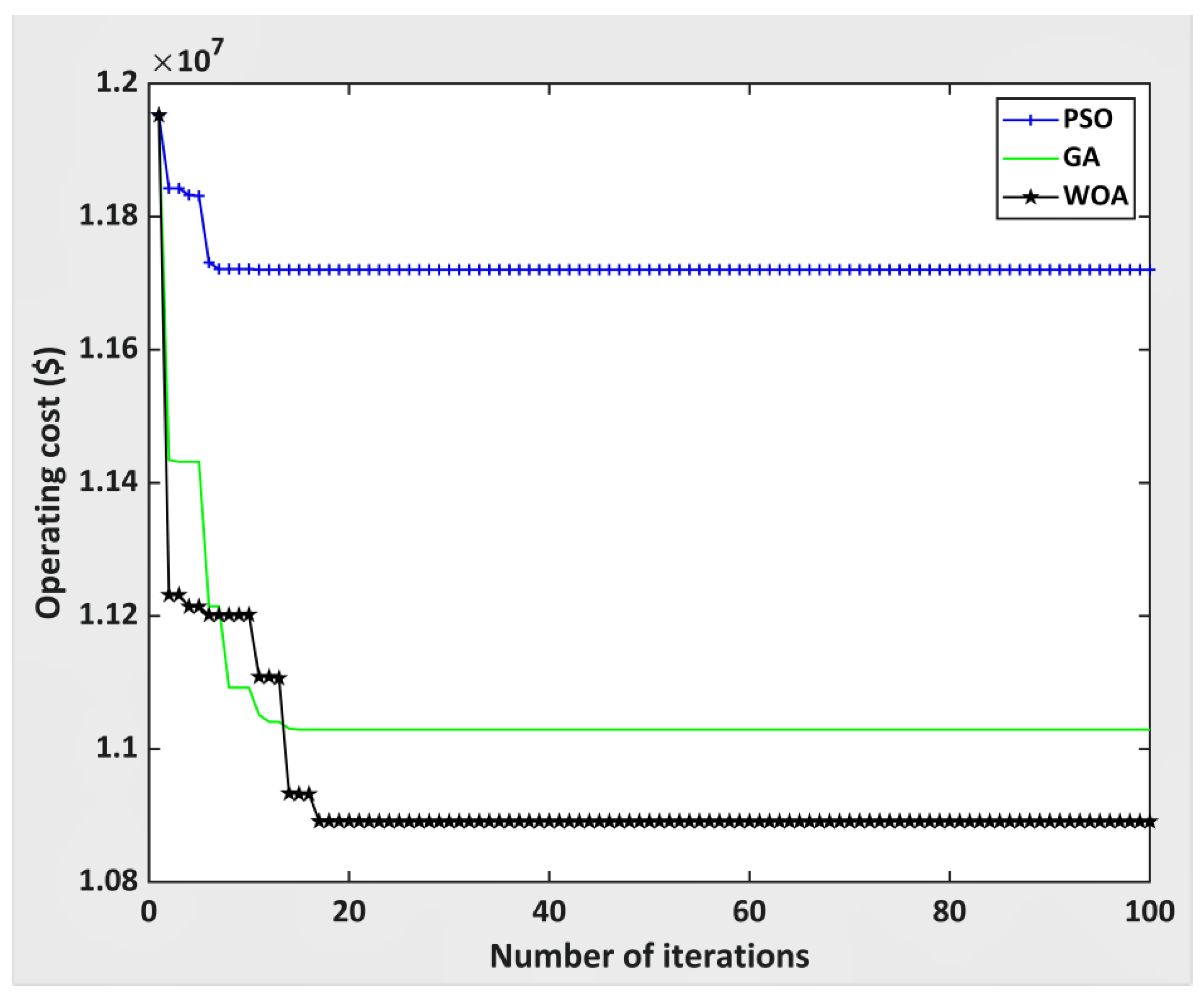
| 200 | 1.1952 × 10⁷ | PSO | 3.433 × 10⁵ | 1.172 × 10⁷ |
| GA | 2.988 × 10⁵ | 1.1029 × 10⁷ | ||
| WOA | 2.870 × 10⁵ | 1.0891 × 10⁷ | ||
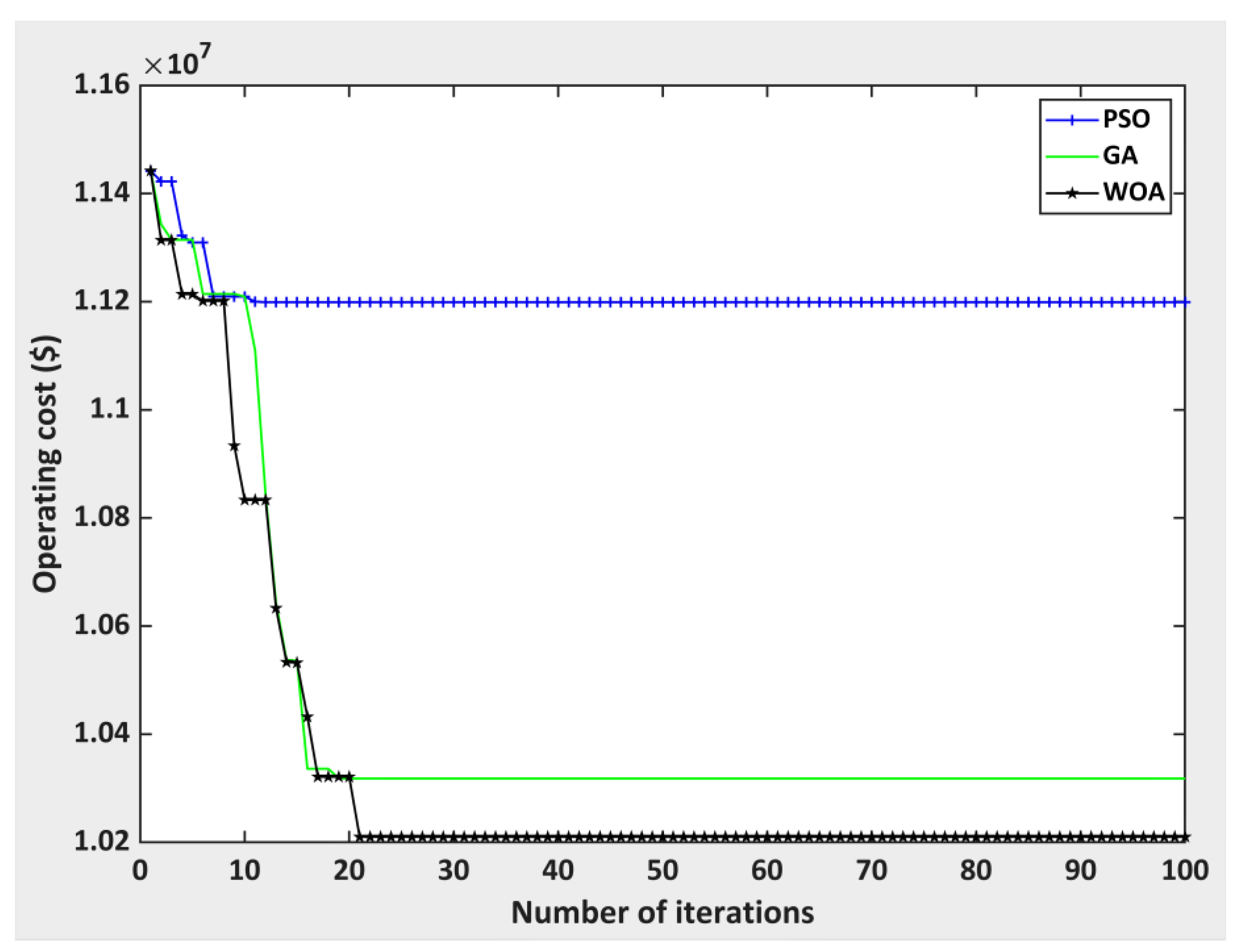
| 150 | 1.1442 × 10⁷ | PSO | 3.033 × 10⁵ | 1.1199 × 10⁷ |
| GA | 2.580 × 10⁵ | 1.0318 × 10⁷ | ||
| WOA | 2.525 × 10⁵ | 1.021 × 10⁷ | ||
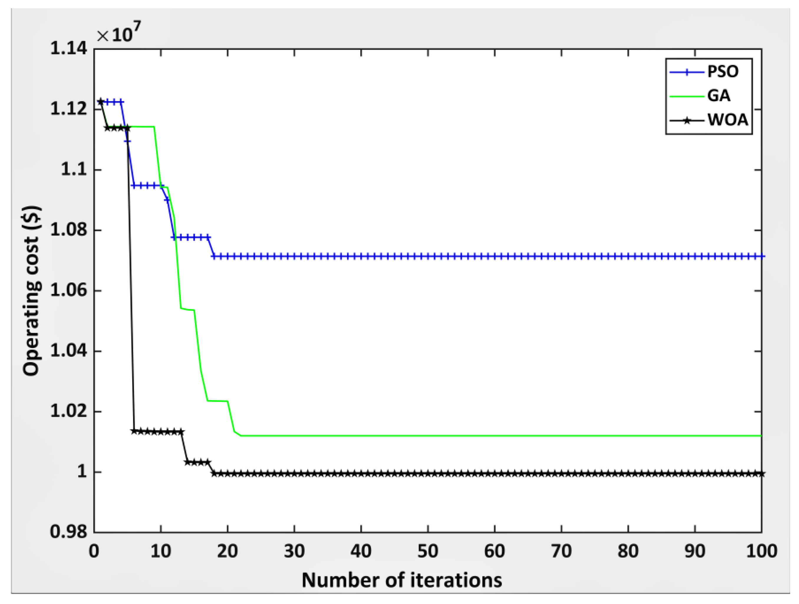
| 100 | 1.1226 × 10⁷ | PSO | 3.677 × 10⁵ | 1.0714 × 10⁷ |
| GA | 3.202 × 10⁵ | 1.012 × 10⁷ | ||
| WOA | 2.424 × 10⁵ | 0.9995 × 10⁷ |
| Fitness Function Variables | Optimal Settings at 200% Reactive Loading (p.u) | Optimal Settings at 150% Reactive Loading (p.u) | Optimal Settings at 100% Reactive Loading (p.u) | ||||||
|---|---|---|---|---|---|---|---|---|---|
| PSO | GA | WOA | PSO | GA | WOA | PSO | GA | WOA | |
| SVC (7) | 0.003 | 0.201 | 0.041 | 0.051 | 0.160 | 0.029 | 0.011 | 0.090 | 0.001 |
| SVC (9) | 0.022 | 0.170 | 0.034 | 0.012 | 0.120 | 0.290 | 0.061 | 0.052 | 0.001 |
| SVC (11) | 0.194 | 0.112 | 0.005 | 0.125 | 0.070 | 0.094 | 0.002 | 0.040 | 0.061 |
| SVC (14) | 0.127 | 0.061 | 0.002 | 0.102 | 0.102 | 0.081 | 0.194 | 0.150 | 0.001 |
| TCSC (8) | 0.001 | 0.014 | 0.050 | 0.086 | 0.124 | 0.005 | 0.034 | 0.102 | 0.060 |
| TCSC (9) | 0.002 | 0.008 | 0.050 | 0.018 | 0.001 | 0.059 | 0.011 | 0.016 | −0.040 |
| TCSC (15) | 0.014 | 0.024 | 0.061 | 0.000 | 0.067 | 0.073 | 0.040 | 0.043 | 0.051 |
| TCSC (18) | 0.001 | 0.000 | 0.019 | 0.001 | 0.017 | 0.000 | 0.001 | 0.011 | 0.091 |
| UPFC (3) | 0.006 | 0.019 | 0.004 | 0.000 | 0.008 | 0.031 | 0.170 | 0.001 | 0.001 |
| UPFC (2) | 0.280 | 0.000 | 0.001 | 0.002 | 0.009 | 0.001 | 0.003 | 0.039 | 0.100 |
| UPFC (5) | 0.001 | 0.001 | 0.009 | 0.070 | 0.001 | 0.311 | 0.000 | 0.002 | 0.000 |
| QG (2) | 0.122 | 0.154 | 0.601 | 0.015 | 0.681 | 0.600 | 0.312 | 0.613 | 0.551 |
| QG (3) | 0.321 | 0.277 | 0.581 | 0.419 | 0.083 | 0.369 | 0.389 | 0.667 | 0.481 |
| QG (6) | 0.415 | 0.091 | 0.182 | 0.225 | 0.184 | 0.487 | 0.413 | 0.519 | 0.101 |
| QG (8) | 0.087 | 0.623 | 0.163 | 0.451 | 0.212 | 0.098 | 0.513 | 0.082 | 0.682 |
| TAP (8) | 0.982 | 1.018 | 0.900 | 0.913 | 0.976 | 1.0300 | 0.905 | 1.054 | 0.901 |
| TAP (9) | 0.995 | 0.919 | 0.991 | 0.985 | 0.992 | 0.902 | 0.991 | 0.981 | 0.978 |
| TAP (10) | 0.957 | 0.996 | 0.985 | 0.996 | 1.000 | 1.013 | 0.916 | 0.985 | 0.901 |
| Percentage Reactive Loading | Total Cost of Power Loss of System (A) ($) | Algorithm Used to Minimize Objective Function | FACTS Devices Cost ($) | Operating Cost with FACTS (B) ($) |
|---|---|---|---|---|
| 200 | 1.4902 × 10⁷ | PSO | 3.774 × 10⁵ | 1.393 × 10⁷ |
| GA | 3.517 × 10⁵ | 1.325 × 10⁷ | ||
| WOA | 3.527 × 10⁵ | 1.318 × 10⁷ | ||
| 150 | 1.443 × 10⁷ | PSO | 3.479 × 10⁵ | 1.3601 × 10⁷ |
| GA | 3.082 × 10⁵ | 1.215 × 10⁷ | ||
| WOA | 3.028 × 10⁵ | 1.205 × 10⁷ | ||
| 100 | 1.4152 × 10⁷ | PSO | 3.136 × 10⁵ | 1.266 × 10⁷ |
| GA | 2.908 × 10⁵ | 1.177 × 10⁷ | ||
| WOA | 2.791 × 10⁵ | 1.1703 × 10⁷ |
| Fitness Function Variables | Optimal Setting at 200% Reactive Loading | Optimal Setting at 150% Reactive Loading | Optimal Setting at 100% Reactive Loading | ||||||
|---|---|---|---|---|---|---|---|---|---|
| PSO | GA | WOA | PSO | GA | WOA | PSO | GA | WOA | |
| SVC (26) | 0.041 | 0.045 | 0.057 | 0.051 | 0.031 | 0.049 | 0.021 | 0.032 | 0.000 |
| SVC (29) | 0.194 | 0.211 | 0.049 | 0.143 | 0.117 | 0.240 | 0.078 | 0.046 | 0.010 |
| SVC (30) | 0.142 | 0.108 | 0.0418 | 0.072 | 0.093 | 0.140 | 0.055 | 0.048 | 0.018 |
| TCSC (15) | 0.026 | 0.014 | 0.050 | 0.086 | 0.124 | 0.005 | 0.034 | 0.102 | 0.060 |
| TCSC (7) | 0.015 | 0.024 | 0.061 | 0.000 | 0.067 | 0.073 | 0.040 | 0.043 | 0.051 |
| TCSC (20) | 0.048 | 0.008 | 0.050 | 0.018 | 0.001 | 0.059 | 0.011 | 0.016 | −0.040 |
| UPFC (3) | 0.018 | 0.011 | 0.241 | 0.011 | 0.028 | 0.051 | 0.017 | 0.011 | 0.041 |
| UPFC (6) | 0.003 | 0.034 | 0.004 | 0.037 | 0.005 | 0.031 | 0.023 | 0.013 | 0.041 |
| UPFC (4) | 0.025 | 0.028 | 0.031 | 0.024 | 0.009 | 0.051 | 0.016 | 0.037 | 0.001 |
| QG (2) | 0.318 | 0.158 | 0.590 | 0.267 | 0.042 | 0.131 | 0.198 | 0.267 | 0.610 |
| QG (5) | 0.248 | 0.103 | 0.290 | 0.364 | 0.698 | 0.591 | 0.014 | 0.388 | 0.509 |
| QG (8) | 0.023 | 0.191 | 0.501 | 0.611 | 0.045 | 0.610 | 0.581 | 0.314 | 0.098 |
| QG (11) | 0.518 | 0.208 | 0.191 | 0.317 | 0.142 | 0.519 | 0.318 | 0.301 | 0.611 |
| QG (13) | 0.032 | 0.605 | 0.189 | 0.345 | 0.298 | 0.181 | 0.676 | 0.097 | 0.184 |
| TAP (11) | 0.914 | 0.904 | 1.034 | 0.982 | 0.914 | 0.991 | 0.948 | 0.903 | 1.032 |
| TAP (12) | 1.038 | 0.981 | 1.050 | 0.938 | 0.901 | 0.990 | 0.934 | 1.012 | 0.920 |
| TAP (15) | 0.902 | 0.958 | 1.043 | 0.984 | 0.918 | 1.020 | 0.931 | 0.907 | 1.018 |
| TAP (36) | 0.918 | 0.905 | 0.988 | 0.901 | 0.926 | 1.038 | 0.938 | 0.994 | 0.991 |
© 2020 by the authors. Licensee MDPI, Basel, Switzerland. This article is an open access article distributed under the terms and conditions of the Creative Commons Attribution (CC BY) license (http://creativecommons.org/licenses/by/4.0/).
Share and Cite
Nadeem, M.; Imran, K.; Khattak, A.; Ulasyar, A.; Pal, A.; Zeb, M.Z.; Khan, A.N.; Padhee, M. Optimal Placement, Sizing and Coordination of FACTS Devices in Transmission Network Using Whale Optimization Algorithm. Energies 2020, 13, 753. https://doi.org/10.3390/en13030753
Nadeem M, Imran K, Khattak A, Ulasyar A, Pal A, Zeb MZ, Khan AN, Padhee M. Optimal Placement, Sizing and Coordination of FACTS Devices in Transmission Network Using Whale Optimization Algorithm. Energies. 2020; 13(3):753. https://doi.org/10.3390/en13030753
Chicago/Turabian StyleNadeem, Muhammad, Kashif Imran, Abraiz Khattak, Abasin Ulasyar, Anamitra Pal, Muhammad Zulqarnain Zeb, Atif Naveed Khan, and Malhar Padhee. 2020. "Optimal Placement, Sizing and Coordination of FACTS Devices in Transmission Network Using Whale Optimization Algorithm" Energies 13, no. 3: 753. https://doi.org/10.3390/en13030753
APA StyleNadeem, M., Imran, K., Khattak, A., Ulasyar, A., Pal, A., Zeb, M. Z., Khan, A. N., & Padhee, M. (2020). Optimal Placement, Sizing and Coordination of FACTS Devices in Transmission Network Using Whale Optimization Algorithm. Energies, 13(3), 753. https://doi.org/10.3390/en13030753