Abstract
Turbomachinery has been widely used in the energy systems as an energy conversion device, such as gas turbine and aero-engine. The losses in the turbomachinery, especially in the multi-stage conditions, restrict the energy conversion efficiency and corresponding fuel economy. Previous studies show that non-axisymmetric endwall could be used to decrease the losses in compressors, but the real effects in the rig tests are usually inconsistent with the numerical simulation. In this paper, a shroud profiled endwall optimization method with the strategy of local loss as the objective function is proposed, aiming at reducing the tip loss of an embedded stator under the operating point. The traditional total loss coefficient and four local loss functions are studied to investigate how the objective functions influence the optimization results. Three optimized endwall geometries are tested in the embedded test platform. It showed that the strategy of loss coefficient above 90% span as the objective function was best at decreasing the stator loss in the tip region as well as the whole span. Under this strategy, the loss above 90% span was suppressed by 48.17% and the loss of the whole span decreased 9.27%, which proved the PEW optimization design method with the strategy of local loss as the objective function is potential.
1. Introduction
Non-axisymmetric endwall is first used in the turbines to make the flow field of stator more uniform and reduce the secondary flow losses [1,2]. Non-axisymmetric endwall used in compressors is not as effective as in the turbines, which owing to the circumferential pressure gradient between the PS (pressure side) and SS (suction side) of the blade passage in the compressor is lower than that in the turbines [3]. Also, the inverse pressure gradient along the flow direction in the compressor is easy to cause a separation, which means that the endwall profiling should pay more attention to achieving a positive gain of the performance.
Profiled endwall (PEW) has been widely studied in the compressors and turbines, both numerically and experimentally [1,2,3,4,5,6,7,8,9,10], with its direct effect on the flow field near the endwall region and further influence on the main flow. Rose [1] proposes the PEW with the form of non-axisymmetric and explains the mechanism of PEW on depressing the corner separation, that it relieves the pressure gradient of endwall from PS to SS and weakens the secondary flow near the endwall [2]. Tests conducted by Harvey on linear compressor cascade show that the numerical calculation has overestimated the benefits of the PEW with respect to the exit whirl angle [3]. Further CFD calculations indicate that the PEW could achieve similar effects as the 3-D blading [4]. Reising [5,6] proposes that enhanced crossflow from PS to SS caused by the PEW helps to suppress the endwall separation, which is contrary to the conventional explanation for the effect of the PEW. Investigations on the mechanism of how the PEW improves the blade performance are still ongoing.
When the PEW applies to the casing, it is similar to a casing treatment technology. The common casing treatment always contains some grooves or slots, whether stream-wise or circumferential, makes the endwall to be a discontinuous surface [11,12,13,14]. Similarly, the non-axisymmetric endwall in the shroud could be considered as a kind of casing treatment with a continuous surface consists of concave and convex zones. Casing treatment could suppress the tip leakage vortex in the tip region of the rotor by inducing local circumferential or radial velocity. The profiled endwall mainly changes the distribution of the static pressure and controls the secondary flow by modifying the streamline curvature near the endwall.
PEW is generated mainly by two means. One is control lines with two crossed directions with functional expressions [1,2], which is called function modeling method and the other one is applying perturbations to the discrete points within the profiled zone [5,6,7,8,9], which is called perturbation method. The former one often chooses trigonometric functions and B-spline curves as the control function. The number of control variables is often fewer than the latter method. It often chooses some typical values of control variables and conducts the CFD simulation. By comparing the simulation results, optimum values of the variables were got to give a reference to practical engineering. The latter one can introduce more design variables and make the PEW have more degree of freedom. The optimization design method often adopts the perturbation method, as it has more freedom than the function modeling method, which could explore more probabilities of the effects of PEW on improving the flow field.
However, most of the studies of PEW concentrate on the cascade or single stage [5,6,7,8,9], and fewer investigations on the multistage conditions, which are due to the complicated flow structures of the multistage turbomachinery. A troublesome problem is that the test results could not show as effective as the numerical simulation predicted, which has been reported in the previous papers [3,4]. Experimental study is crucial when applying PEW on the engineering practice as CFD simulation could hardly predict the precise flow fields in the multistage condition.
In this paper, the stator of the 3rd stage in a 4.5-stage compressor is chosen as the prototype stator. The simulation results of the outlet total pressure contour for the prototype stator coincident well with the test results. Then a surrogate-based optimization (SBO) is performed on the prototype stator. Five optimization schemes are proposed with different objective functions and three of the optimization results are tested. It shows that choosing the local loss coefficient from 90% to 100% span as the objective function is better than the traditional total loss coefficient of the whole blade height in reducing the loss of the stator. The mechanism of how the profiled endwall influence the flow field is discussed according to the test results.
2. Research Object and Test Platform
2.1. Research Object
The test rig was a low-speed research compressor (LSRC), as shown in Figure 1. It was a 4.5-stage repeated compressor with inlet guide vanes and four repeated stages. The detailed parameters of the compressor were listed in Table 1.
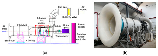
Figure 1.
4.5-stage low-speed research compressor (LSRC) test rig in NUAA (2018). (a) A sketch of compressor test rig (b) Photograph of the LSRC test rig.

Table 1.
Global parameters of the LSRC (2018) in NUAA.
The test configuration was shown in Figure 2. There were 11 test planes distributed along the compressor, denoted from “A-A” to “L-L.” Six total pressure pneumatic probes, six static pressure holes on the casing and eight static pressure holes on the hub were uniformly mounted at plane A-A respectively. The average total pressure and static pressure was used to calculate the mass-flow rate of the compressor. Similarly, eight total pressure pneumatic probes, eight static pressure holes on the casing and eight static pressure holes on the hub were uniformly mounted at plane L-L respectively. Two boundary layer probes were mounted on the hub and casing at plane A-A respectively. From plane B-B to J-J, eight total pressure probes and eight static pressure holes on the casing were uniformly mounted. The test probes and holes of the A-A and L-L plane were always mounted to monitor the performance of the compressor and the other planes are optional which depended on the test requirement. The descriptions of the total pressure pneumatic probes and boundary layer taps could be found in the previous works of our lab [15,16,17,18].
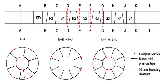
Figure 2.
Test configurations of the compressor rig.
The performance of the compressor was obtained from the inlet A-A plane and outlet L-L plane, and the pressure rise and efficiency characteristic maps were shown in Figure 3. Flow coefficient , total pressure rise coefficient and total to total isentropic efficiency of the compressor were defined as Equations (1)–(7). The blue lines stand for the results of January 18 in 2018 and the green lines stand for the results of August 24 in 2019. Figure 3 shows that the compressor works with a stable performance that the characteristic lines have little variation in over one and a half years.
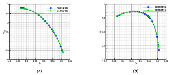
Figure 3.
Performance of the LSRC. (a) Total pressure rise coefficient versus flow coefficient. (b) Total to total isentropic efficiency versus flow coefficient.
As Figure 4 shows, there are nine test slots distributed on the casing that are used to install the displacement controllers for detailed tests of every rotor-stator interface plane, corresponding to the positions of the planes from “B-B” to “K-K” in Figure 2. The detailed tests were conducted by four-hole pneumatic probes, which were driven by the displacement controllers, in the fixed reference frame. More descriptions about the four-hole pneumatic probes and tests for a detailed flow field between two adjacent rows could be found in [15,16,17,18].
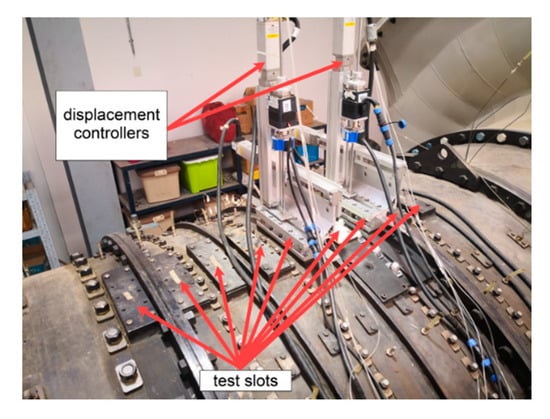
Figure 4.
Test slots distribution and the displacement controllers mounted upon.
The absolute Mach number contours from the inlet of R1 to the outlet of S4 at the design point are shown in Figure 5. From the test results, we can see the development of the flow. The flow field of each rotor outlet shows a circumferential non-uniformity, which becomes more and more severe when it flows downstream. The flow field of each stator outlet shows that the width of the wake in the tip is wider than in the hub, which indicates that the tip region undergoes a worse condition.
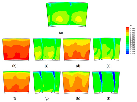
Figure 5.
Absolute Mach number contours at the design point. (a) Inlet of R1; (b) Outlet of R1; (c) Outlet of S1; (d) Outlet of R2; (e) Outlet of S2; (f) Outlet of R3; (g) Outlet of S3; (h) Outlet of R4; (i) Outlet of S4.
The test result of circumferential non-uniformity of the rotor outlet is not occasional. It has been reported by Liu [19] in a one-stage compressor with IGV, which was tested in the fixed frame by a 5-hole pneumatic probe downstream of the rotor row. Liu explains the uniformity is caused by rotor tip separation and the corresponding blockage, and then the flow field could not be simply mixed to be homogeneous in a limited axial distance from the rotor trailing edge to the downstream stator leading edge, which would be more severe when it comes to the near stall condition [19]. In this 4.5-stage test rig, every rotor outlet experiences a similar blockage as the 1.5-stage rig mentioned above. The difference is that the multistage condition makes the blockages of the rear rotors more and more severe, as the normalized axial velocity contours shown in Figure 6. The normalized axial velocity is defined by
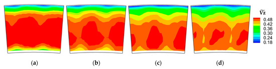
Figure 6.
Normalized axial velocity contours of each rotor outlet. (a) R1 Outlet; (b) R2 Outlet; (c) R3 Outlet; (d) R4 Outlet.
The blockage is apparent in the rotor of the second stage (R2) and more and more severe as propagating downstream. The separation of the stators couples with the formation of the rotor blockage in the multistage condition. The stator tip separation causes the deficit of through-flow capability in the tip region of the downstream rotor blade row and a larger incidence angle that induces the rotor tip separation and blockage. The blockage in the rotor tip region further increases the incidence angle of the downstream stator, which would cause a severer separation than the stator of the prior stage.
As Figure 5 shows, the outlet of S3 exhibits a tip separation, which is severer than the outlet of S2. Similarly, the outlet of S4 exhibits a severer separation than outlet of S3. S3 experiences a median separation contrast with S2 and S4. If the separation of S3 being suppressed, then the downstream flow condition would be improved and the performance of the whole stage would be better. Then S3 was chosen as the research object. S3 experienced the inlet condition of tip blockage (as shown in Figure 5f and Figure 6c) and outlet condition of tip separation (as Figure 5g shows), which is a representative condition of an embedded stator in the multistage axial compressor. The aim of the study is to depress the tip separation of S3 by endwall profiling. The study is meaningful to the practical engineering as it could give a reference to the modification of the middle stage. It is also a challenging work as the embedded stator is influenced by the upstream and downstream rotors, which are both strongly unsteady and combined with the propagation of the wakes of each blade row.
2.2. Test Platform
An annular sector cassette was designed and applied in the stator row of the third stage, as illustrated in Figure 7. Compared with the linear cascade, the sector cassette could keep the unsteady condition induced by the upstream and downstream rotors. The advantage of the sector cassette is the quick change of eight modified blades rather than 84 blades in the full annulus. The insertion of cassettes with modified geometries makes the disassembly and assembly of the test facility more convenient, compared with the disassembly and assembly of the whole compressor to change the blades. It is easy to install the sector cassette into the casing with the help of a gantry crane. The disadvantage is that it could not test the performance maps of the compressor as it did not change the full annular blades. It can test at the same operating point as the prototype compressor.
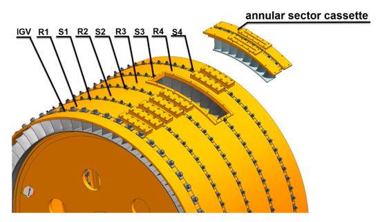
Figure 7.
A sketch of the annular sector cassette test platform.
The annular sector cassette was designed with a cavity of 10 mm inward the casing, which allowed changing different PEWs, as Figure 8a shows. 3-D printing technology was introduced to manufacture blades and PEWs in the annular sector cassette, instead of the traditional metal processing. For the consideration of constructing a whole blade passage, the blades and PEWs are not printed one by one, but in sets of 4 or 2, as Figure 8b shows. The PEWs and blades are assembled with casing as Figure 8c shows.
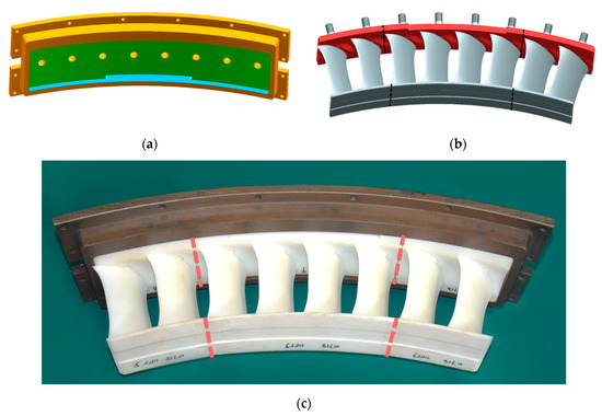
Figure 8.
Design of the annular sector cassette. (a) CAD model of sector casing with cavity. (b) CAD model of blades and Profiled endwall (PEWs). (c) Photograph of the annular sector cassette with PEWs and blades.
The 3-D printer is an industrial stereo lithography apparatus (SLA) printer and the material is photosensitive resin. The spatial resolution is 0.1 mm, which is enough for the stator blades with a span height of 90 mm and a chord length of approximately 80 mm. The smoothness of the blade is well enough for the tests in the compressor without the need for post-processing. The cost of each blade is only 10 percent of a traditional metallic one. A group of blades with PEWs for the annular sector cassette could be printed within 10 h. It greatly reduces the manufacturing time and costs, which contributes significantly to the aim of low-cost and time-saving tests. The stators have a full hub which means that the bending deflection is weak and the mechanical strength is enough, which has been tested for hundreds of hours.
3. Numerical Setup
The optimization design of the PEW was based on CFD. Numerical simulations were conducted by commercial software NUMECA 13.2, which contained the construction of the grid file, the calculation of the flow field and the post-processing to obtain the performance of the compressor.
The grid file was generated by the Autogrid5 module, with the inlet and outlet of the compressor set to be two times of stator chord length respectively, as Figure 9 shows. O4H topology was applied in the main flow region, and butterfly topology was used in the rotor tip gap. The whole grid contains 71 blocks. The first layer grid thickness against the solid wall was 4 × 10⁻⁶ m, to ensure that the y+ is no more than 4. The solid boundaries were all set to be no-slip and adiabatic. Four sets of grid configurations were applied to investigate the grid sensitivity. Detailed data for each configuration are given in Table 2.
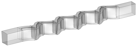
Figure 9.
Block distribution for the 4.5 stage compressor.
Table 2.
Names of optimization schemes for each objective function and the baseline values.
Three-dimensional viscous CFD single-passage computation was performed by flow solver EURANUS on the LSRC to contrast with the experimental characteristic curve. The governing equations were Reynolds-Averaged Navier-Stokes (RANS) equations. Spalart-Allmaras (SA) turbulence model was chosen to estimate the eddy viscosity coefficient. The inlet condition was set to be axial inflow with a standard atmospheric environment. CFL number was set to 3. The outlet condition was set at midspan and governed by radial equilibrium equations. A throttling process was simulated by increasing the outlet static pressure.
The pressure rise and efficiency characteristic maps of the simulation were contrasted with the test results in Figure 10. Grid g1 had the biggest variance of these four schemes. When the grid got denser from g2 to g4, the pressure rise and efficiency changed little, but the stall margin decreased. Grid g2 was best at balancing the time cost and simulation accuracy. Under grid g2, the simulation results could get a good prediction of the compressor performance.
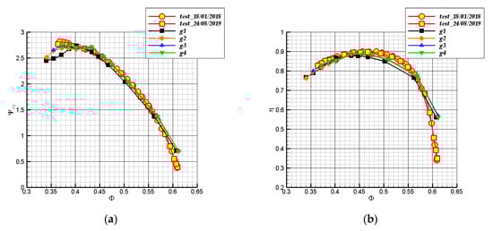
Figure 10.
The numerical results and test data. (a) Pressure rise characteristic; (b) total to total isentropic efficiency characteristic.
However, the simulation of the whole compressor with 4.5 stages is time-consuming and unpractical in engineering for the optimization. An attempt was made that only conduct the optimization on the third stage at the design point (DP) of the compressor. The grid configuration of the third stage was the same with g2 except the inlet and outlet positions were 1 time of the chord length of the stator. The inlet condition of the third stage was given by a radial distribution of total pressure and velocity directions obtained from the test results at the design point. The outlet condition was given by a mass flow rate value, which could guarantee that all of the revised blades had the same operating condition with the prototype blade. This was a test-related numerical method, as the boundary conditions were given according to the test results. The normalized total pressure is defined by Equation (9), where is the mass-averaged total pressure of the plane,
and is the mass-averaged density of the plane. Test results of the inlet and outlet of S3 are shown in Figure 11a,c, and simulated results are shown in Figure 11b,d. The contours of simulation at the inlet and outlet of S3 fitted well with the test results, which means the blockage phenomenon behind the rotor has been taken into account in the optimization.
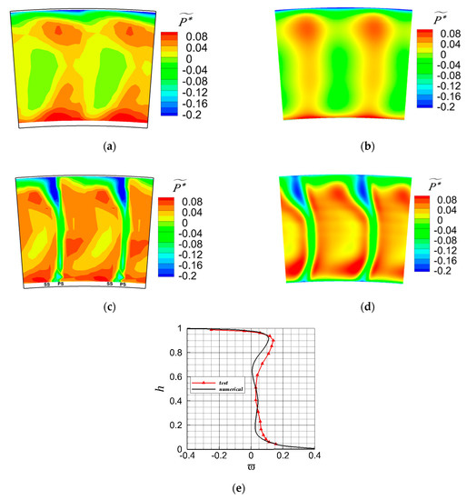
Figure 11.
Test and numerical results of the third stator. (a) Normalized total pressure contour of the stator inlet of the test results. (b) Normalized total pressure contour of the stator inlet of the numerical results. (c) Normalized total pressure contour of the stator outlet of the test results. (d) Normalized total pressure contour of the stator outlet of the numerical results. (e) Comparison of the distribution of the total loss coefficient of test and numerical results.
The total pressure loss coefficient is defined as Equation (10), where h is the relative blade height ranged from 0 to 1, corresponding to the blade hub to the shroud. Figure 11e gives the comparison of loss distribution of the simulation and test results. The maximum value in the upper half of the loss profile appears at 0.9h, which corresponding to the core of the low-pressure zone. Though the total pressure loss coefficient obtained from the numerical simulation was lower than the tested one, it can give a qualitative prediction, especially the maximum loss position, which indicates that it was possible to perform a PEW optimization on S3. As can be seen in Figure 11c,d, the low-pressure zone in the tip region covered about 30% blade height. The form of the separation zone indicated that it was a blade separation rather than a corner separation. The blockage in the tip region of R3 increased the incidence angle of S3 and the blade load, which lead to the blade separation in the tip of S3 outlet. The loss coefficient above 0.6h was higher than the mainflow because of the blade separation. The maximum loss appeared at 0.9h where the separation is severest in this position.
The simulation of one stage could significantly reduce the optimization time and keep the main flow features. It should be noticed that the research object is still only S3, but the whole third stage is selected to conduct the simulation to guarantee the inlet of S3 fits well with the engine-realistic flow condition.
4. Optimization Design and Experimental Study
4.1. Optimization Design
4.1.1. Optimization Design Platform
FINETM/Design3D integrates a new optimization kernel Minamo, developed by Cenaero, from version 13.1. It offers best-in-class global optimization methods with superior auto-adaptive space filling techniques, highly efficient non-linear surrogate models and advanced genetic algorithms to drive the optimization process [20]. An SBO method was applied to conduct the profiling of the shroud endwall. The optimization results of the SBO method are determined by three key elements: the design of experiment (DoE), the surrogate model, and the optimization algorithms. The DoE technique ensures that the surrogate model to be well constructed under a finite number of samples. The surrogate model contains the response surface methodology (RSM), Kriging model, artificial neural network (ANN), and radial basis function network (RBFN), and so on. The optimization algorithms include the genetic algorithms, the gradient algorithms, and simulated annealing algorithms, etc. In this paper, the SBO method employed the Latinized Centroidal Voronoi Tessellations (LCVT) technique in the DoE process, the RBFN as the surrogate model and the genetic algorithms as the optimization algorithm.
The optimization process contained three steps, namely the parametric modeling of the shroud profiled endwall (SPEW), the CFD simulation settings (including the grid generation, boundary conditions, initial solutions, the turbulence model and so on), and the surrogate-based genetic-algorithm optimization.
A SPEW parametric modeling method was developed by parameterizing the shroud surface with 48 discrete points homogeneously distributed and applying radial perturbations on the discrete points. The profiled zone was limited from the leading edge to the trailing edge of the stator in the axial direction and between two camber lines in the circumferential direction, as Figure 12a shows. Six Bezier curves along the flow direction (blue lines in Figure 12a,b) and eight Bezier curves along the circumferential direction (pink lines in Figure 12a,b) were applied to construct a smooth surface. The six control lines along the flow direction were homogeneously set from PS to SS and each line was controlled by eight equidistant points. There were only five real control lines as the two boundary control lines are periodic which used the same control parameters. Then the number of variable points decreases to 40. The control lines were defined to be Bezier curves and vary with the amplitude of the control points. Considering the inlet and outlet of the profiled surface to smoothly connected with the axisymmetric surface, the amplitudes of the radial perturbations of the first and the last point for each line (as black points in Figure 12b,c shows) were set to be 0 to ensure C0 continuity, and the second and the last but one points (as green points in Figure 12b,c shows) were adapted to make the slopes of the first and the last point to be 0 to ensure G1 continuity. Then the number of control points decreased to 20 (as the red points in Figure 12b shows), and the amplitudes of these 20 points were the design parameters. The blade height was 90 mm, and the amplitude was set to be ±6 mm, which accounts for about 6.67% of the blade height. The number of design parameters was limited to ensure the surrogate model to be well constructed under a finite number of samples.
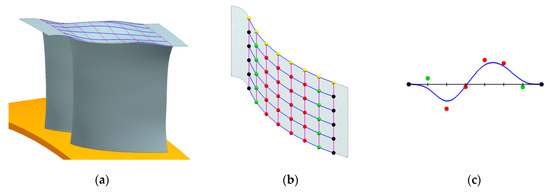
Figure 12.
Parametric modeling of the stator shroud. (a) Illustration of the non-axisymmetric endwall of the stator shroud. (b) Distribution of the control points. (c) Amplitude of the control point and the corresponding Bezier curve.
The CFD simulation settings were set according to the prior section, which fitted well with the test results for the prototype stator at the operating point. The grid of the shroud endwall was added to S3 by the Autogrid5 module.
The surrogate-based-genetic-algorithm was chosen here as it could sharply decrease the optimization time. The surrogate model was constructed by RBFN, which could predict the CFD results more and more accurate with the number of the CFD results increasing in the database. Generally, the genetic algorithm (GA) conducted a certain number of generations, and each generation consisted of a fixed number of individuals (here an individual contains the geometric parameters and the related CFD responses for a given SPEW geometry). The total time of the optimization would be months if each individual was calculated by CFD simulation. A finite number of existing individuals (usually more than 2 times of the design parameters) were used to train the RBFN model and get a surrogate model to predict the response for a new individual instead of the CFD simulation. Each individual was calculated by the surrogate model in one generation, and the optimum one in this generation was chosen to conduct the CFD simulation, with the CFD responses adding to the database to further train the surrogate model, which sharply decreased the consuming time for each generation. Then the refined surrogate model was used to conduct the GA optimization of the next generation. The detailed process diagram is shown in Figure 13.
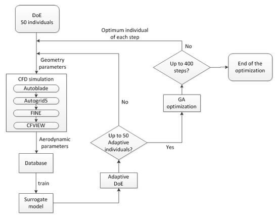
Figure 13.
Scheme of the MINAMO optimization integrated in the Design3d module.
First, an initial database containing 50 individuals was generated through DoE. This is a priori sample process, with the LCVT technique to guarantee both discrepancy and volumetric uniformity. The database was used to build an analytical relationship between the design parameters (part of the geometry parameters) and simulation responses (aerodynamic parameters), namely the process of constructing the surrogate model. The surrogate model implied a tuned RBFN to minimize the error between the CFD simulation outputs and the predicted results of the surrogate model by adjusting the values of the weights, which is called training of the surrogate model.
Then 50 adaptive DoE individuals were conducted to enlarge the database where the responses changed significantly, with the purpose of covering more points in the design space. The surrogate model first selects a set of geometric parameters as one individual that could severely influence the response predicted by the model, followed by a CFD simulation to measure the error between the predicted response and the CFD simulation result, and then the surrogate model would adjust the values of the weights to fit with the CFD response. This procedure was the so-called posteriori sequential sample, compared with the priori sample mentioned above.
Finally, 400 steps of optimization were performed to get an optimum solution. Every step (an optimization recycle is one step) contains training of the surrogate model, a GA optimization and a CFD simulation. One GA optimization contains 100 generations, and every generation contains 400 individuals which are predicted by the surrogate model rather than CFD simulation. After the GA optimization, the best individual was chosen to perform a CFD simulation. The CFD response was put into the database to further train the surrogate model.
4.1.2. Optimization Objective Functions
The conventional objective functions for the optimization are usually the total characteristic of the blade, such as the stage efficiency, the rotor pressure rise ratio, the stator loss and so on, which measures the overall performance of the blade, rather than the local characteristics. The outlet total pressure contour of the prototype S3 in Figure 11c shows that there is an apparent low-pressure zone, which is relevant to a tip separation. The local loss coefficient would be a more suitable objective function than the total loss coefficient, as the tip region is the crucial position that we care more about. The total loss coefficient is defined as Equation (11). Here the total loss coefficient denotes the mass-averaged loss value of the whole blade height. Four local loss coefficients, , , of the stator are defined as Equations (12) to (15), which denotes the mass-averaged loss value from relative blade height of 0.9, 0.8, 0.7, 0.6 to blade tip correspondingly.
, , , are used to measure the loss of local blade height that focus on the tip region where tip separation appears. Five optimization schemes with different objective functions, , , , , , to be minimized, are denoted as s1, s2, s3, s4, s5, as listed in Table 3. The baseline values are calculated from the axisymmetric stator. The total loss coefficient is lower than the tip loss coefficients. This is reasonable as the tip region bears a large loading and the loss coefficient is higher than the bottom region, as can be seen in Figure 11e. These local loss coefficients are introduced to the optimization by user-defined macros in the post-processing of the Design3d module.
Table 3.
Names of optimization schemes for each objective function and the baseline values (CFD).
Five SPEW geometries corresponding to different schemes are illustrated in Figure 14. It showed a rule that the smaller the region that the objective function focused on, the larger the amplitude of the profiled zone would be. The largest amplitude for these five schemes appeared at s2, which employed +5.5 mm (about 6.11% of the blade height) near the suction side. It was coincident with the classical profiled endwall in the hub as Figure 15 shows. The curvature of the surface is critical to the enwall flow. A concave curvature could induce a relative diffusion of the flow and increase the local static pressure. A convex curvature could accelerate the flow and decrease the local static pressure. For the hub PEW, the shape of an upslope surface from SS to PS is usually beneficial to the blade performance [21]. Accordingly, the shape would be a downslope when it comes to the shroud PEW. Both the downslope rule for hub PEW and the upslope rule for shroud PEW can reduce the cross-passage pressure gradient and the secondary flow intensity.
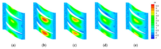
Figure 14.
Geometries of the optimized results. (a) Objective function of; (b) objective function of (c) objective function of ; (d) objective function of (e) objective function of.
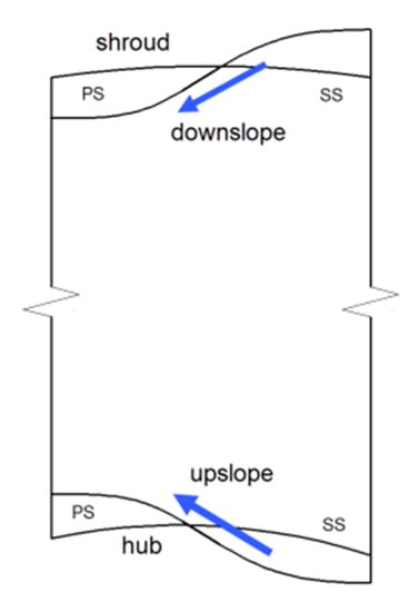
Figure 15.
Sketch of the rules for the profiled endwall.
The changes of different losses for the optimization process under different schemes are illustrated in Figure 16. The DoE process and adaptive DoE process are not presented in the maps and only the optimization process is showed. From the comparison, we can see that the objective function was critical to the optimization results. If the total loss coefficient was chosen as the objective function, it could not directly capture the flow features of the tip region, and make the tip loss larger than the schemes of s2 and s3. In order to reveal the relationship of each loss coefficients in the optimization process, a correlation analysis was performed for each scheme and the results are shown in Table 4. In Table 4b, every correlation factor (CF) is the lowest among these five schemes except the CF of and , which means scheme s2 that focus on the loss above 0.9h is special and requires more attention.
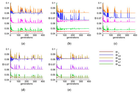
Figure 16.
Changes of different losses during the process of the SPEW optimization with different schemes. (a) Scheme s1; (b) scheme s2; (c) scheme s3; (d) scheme s4; (e) scheme s5.
Table 4.
Correlation factors of each loss coefficients under different optimization schemes. (a) Scheme s1; (b) scheme s2; (c) scheme s3; (d) scheme s4; (e) scheme s5.
The loss coefficient profiles of the final optimization results for each scheme are shown in Figure 17. It is interesting to see that the tip loss, especially the loss upon 90% span, decreased sharply when the objective functions concentrated on the tip region (schemes s2 and s3), compared with the total loss as the objective function. The total loss for s2 is the largest among these five schemes, as the loss between the 60 to 80% span is larger than the axisymmetric stator, in the sense of CFD simulation.
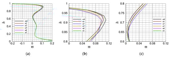
Figure 17.
Comparison of the loss coefficients for the axisymmetric stator (marked as “ori”) and optimization results of different schemes (CFD results). (a) Map for the whole blade height; (b) detailed map that focused on 0.8 to 1 blade height; (c) detailed map that focused on 0.6 to 0.8 blade height.
Table 5 gives the quantitative description of the contrast between the axisymmetric shroud and the optimization results for each loss coefficient under different objective functions. Scheme s1 with the traditional total loss coefficient as the objective function, had the most decreased total loss, from 0.0470 to 0.0432 (relative reduction of 8.0296%), but the tip loss of four different extents,, , , had not decreased too much compared with the objective functions being the corresponding tip loss coefficient. Every optimization scheme could mostly decrease the loss coefficient corresponding to its objective function, as the data marked in bold in Table 5 shown.
Table 5.
Optimization results of the relative reduction values for different loss coefficients under different optimization schemes compared with the axisymmetric shroud stator (CFD results).
4.2. Experimental Study
Experimental studies for the SPEW stator of the middle stage were conducted in the annular sector cassette test platform. Three optimization SPEWs were chosen, namely s1, s2, s5, to conduct the tests.
Figure 18 gives the loss coefficient profiles of the test results for the prototype stator and the optimized stators of different schemes. Table 6 gives the test results of the relative reduction for each loss coefficients. The test results showed some differences with the CFD results. For the CFD results, the loss under 0.5 is nearly the same for each stator. But for the test results, the loss of this extent is different for each scheme. Scheme s1 with the total loss as the objective function makes the loss between 0.25 to the hub of the blade larger than the prototype and the total loss only decreased by 0.34%. For the CFD results, the of scheme s2 is the largest among five optimization schemes, as the loss between 0.6 to 0.8 is larger than the prototype stator. But for the test results, the loss between 0.6 to 0.8 was less than the prototype and the total loss decreased most, up to 9.27% relative reduction.
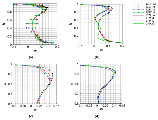
Figure 18.
Comparisons of the loss coefficients obtained from numerical and test results. (a) Test results with error band. (b) Comparison for the numerical and test results of the whole blade height. (c) Test results from 0.6 to the tip of the blade. (d) Numerical results from 0.6 to the tip of the blade.
Table 6.
Optimization results of the relative reduction values for different loss coefficients under different optimization schemes compared with the axisymmetric shroud stator (test results).
Figure 19 gives the outlet normalized total pressure contours for each stator. It showed the application of SPEW to the embedded stator was effective that all three SPEW stators could diminish the tip low-pressure region compared to the prototype blade, corresponding to the lower loss coefficients in the tip region.
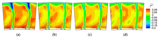
Figure 19.
Total pressure of the stator outlet (test results). (a) Axisymmetric stator; (b) scheme s1; (c) scheme s2; (d) scheme s5.
The secondary flow velocities are defined as the difference between the velocity and the mass-averaged velocity. Figure 20 gives the radial secondary velocity contours together with the secondary velocity vectors consisted of the circumferential secondary velocity and radial secondary velocity . The secondary velocities are defined as Equations (16)–(18), where is
the circumferential velocity and is the radial velocity for every test point, is the mass-averaged circumferential velocity for the corresponding blade height and is the mass-averaged radial velocity for the corresponding blade height, is a 2-D vector with the component of and . The contour maps and secondary velocity vectors indicate that the secondary flow of three SPEW stators in the top half of passage had been suppressed compared with the prototype, which corresponds to the reduction of loss coefficient. The radial secondary velocity toward midspan in the low-pressure zone of blade tip has been enhanced for SPEW stators compared with the axisymmetric stator, especially for scheme s2 which has been highlighted with a red circle in Figure 20c, and the loss coefficient of s2 is the least of these four blades.
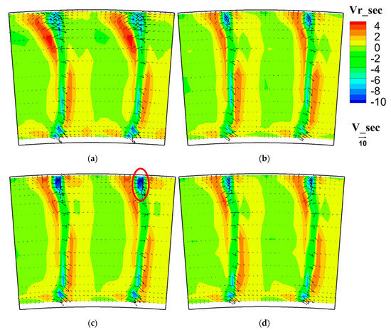
Figure 20.
Secondary velocity contours with secondary velocity vectors (test results). (a) Axisymmetric stator; (b) scheme s1; (c) scheme s2; (d) scheme s5.
A well-designed SPEW (scheme s2) had a direct effect on the flow near the casing and the reduced the secondary intensity near the endwall, but enhanced the radial secondary flow in the shroud/suction corner. The top half of the passage was influenced by the PEW and the secondary flow intensity was relieved, which could reduce the loss in the top half of the blade height. The accumulation in the shroud/suction corner of the low-momentum fluid was relieved because of the reduction of the cross-passage pressure gradient. The well-designed SPEW could also enhance the radial secondary flow which could migrate the low-momentum fluid toward midspan and further decrease the loss coefficient in the tip region.
5. Discussion
The SPEW optimization method with local loss coefficient as objective function applied in the embedded stator of a multistage is effective.
First, the profiling position is determined by the defect of flow field. There is an obvious blade separation in the tip region of the stator outlet and then the profiling position is chosen at shroud rather than hub. Only few PEW performed at shroud in the published papers [5].
Second, the CFD simulation used in the optimization process is a test-related numerical method. The simulation is conducted on one stage, which is the compromise of computational precision and time cost. A 4.5-stage computation can take more factors into consideration but consume more computational time. The inlet condition and outlet mass flow rate is extracted from the test results and the simulation of the baseline stage has a reasonable prediction of the inlet and outlet of S3 in sense of the pressure contour and loss coefficient profile. By applying this test-related simulation method, the differences between the simulation and test results could be minimized for the optimization results. For the optimization with scheme s2, the simulation has successfully predicted that the loss coefficient above 0.85h is lower than the baseline stator.
Third, the local pressure loss coefficient was proposed to be the objective function which is based on the position of blade separation. All the published papers adopt the total performance parameters of the whole blade height as objective functions [5,6,7,8,9], whether single-objective or multi-objective. This paper proposes the performance parameters of local blade height as objective functions and numerically and experimentally studied to validate its advantages over the traditional objective functions.
Finally, the SPEW optimization results with different objective functions have been experimentally studied in the presence of realistic upstream and downstream flow conditions in the multistage compressor test rig. The test results support and validate the optimization with local loss as objective function is effective than the total loss coefficient as objective function in decreasing the stator loss of the tip region as well as the whole blade.
6. Conclusions
In this paper, a method for SPEW optimization of an embedded stator with the strategy of local loss coefficient as the objective function is proposed and the optimization effects are experimentally confirmed in the multistage condition. Five optimization objective functions have been studied and show that the local loss coefficient that concentrates on the tip region of the stator is better at decreasing the tip loss than the traditional objective function of the total loss coefficient. Detailed tests in an annular sector cassette platform show that a well-designed SPEW could decrease the stator loss by relieving the secondary flow intensity in the top half of the passage and migrate the low-momentum fluid toward midspan by enhancing the radial secondary flow in the shroud/suction corner. The test results show that the proposed optimization method is more effective than the traditional objective function of total loss coefficient in decreasing the loss of an embedded stator.
7. Patents
Jun Hu, Jiayu Wang, Chao Jiang, et al. A kind of compressor stator blade fan-shaped section Quick Release housing device [P]. China, Jiangsu Province: CN108953130B, 2019-09-13. (in Chinese)
Author Contributions
Conceptualization, J.W.; methodology, J.W.; software, J.W., C.J., and J.L.; validation, J.W. and J.H.; formal analysis, J.W. and J.H.; investigation, J.W. and C.J.; resources, J.H.; data curation, J.W. and J.L.; writing—original draft, J.W. and C.J.; visualization, J.W. and J.L.; supervision, J.H.; project administration, J.H.; funding acquisition, J.H. All authors have read and agreed to the published version of the manuscript.
Funding
The research presented here was funded by the National Science and Technology Major Project of China, grant number [2017-II-0004-0017].
Conflicts of Interest
The authors declare no conflict of interest.
Nomenclature
| Symbol | Unit | Description |
| () | Area of the annular blade passage | |
| C | Sonic speed | |
| h | (-) | Relative blade height |
| k | (-) | Specific heat ratio |
| Power of isentropic compression consumption | ||
| Power of compressor consumption | ||
| Power of electric motor | ||
| (-) | Mach number | |
| Mass flow rate | ||
| (Pa) | Static Pressure | |
| (Pa) | Total Pressure | |
| Gas constant | ||
| r | (m) | Radius |
| (K) | Static Temperature | |
| (K) | Total Temperature | |
| Blade rotating velocity of midspan | ||
| Axial velocity | ||
| Greek symbols | ||
| (-) | Total to total isentropic efficiency | |
| (-) | Efficiency of the electric motor transport to compressor | |
| Density | ||
| (-) | Total pressure loss coefficient of the stator | |
| (-) | Flow coefficient | |
| (-) | Pressure rise coefficient | |
| Subscripts | ||
| 0.6 | Relative blade height from 0.6 to 1 | |
| 0.7 | Relative blade height from 0.7 to 1 | |
| 0.8 | Relative blade height from 0.8 to 1 | |
| 0.9 | Relative blade height from 0.9 to 1 | |
| A | Plane A-A, Position of compressor inlet | |
| ad | isentropic/adiabatic | |
| C | consumption of the compressor | |
| L | Plane L-L, Position of compressor outlet | |
| m | midspan | |
| n | normalized | |
| Abbreviations | ||
| ANN | Artificial Neural Network | |
| IGV | Inlet Guide Vanes | |
| CFL | Courant-Friedrichs-Lewy | |
| CF | Correlation Factor | |
| CFD | Computational Fluid Dynamics | |
| DoE | Design of Experiments | |
| DP | Design point | |
| GA | Genetic Algorithm | |
| LCVT | Latinized Centroidal Voronoi Tessellations | |
| LSRC | Low-Speed Research Compressor | |
| mm | millimeter | |
| PEW | Profiled Endwall | |
| PS | Pressure surface | |
| RANS | Reynolds-Averaged Navier-Stokes | |
| RSM | Response Surface Methodology | |
| R1 | Rotor of the 1st stage | |
| R2 | Rotor of the 2nd stage | |
| R3 | Rotor of the 3rd stage | |
| R4 | Rotor of the 4th stage | |
| RBFN | Radial Basis Function Network | |
| S1 | Stator of the 1st stage | |
| S2 | Stator of the 2nd stage | |
| S3 | Stator of the 3rd stage | |
| S4 | Stator of the 4th stage | |
| SA | Spalart-Allmaras | |
| SBO | Surrogate-Based Optimization | |
| SLA | Stereo Lithography Apparatus | |
| SPEW | Shroud Profiled Endwall | |
| SS | Suction surface | |
References
- Rose, M.G. Non-axisymmetric endwall profiling in the HP NGV’s of an axial flow gas turbine. In Proceedings of the ASME 1994 International Gas Turbine and Aeroengine Congress and Exposition, The Hague, The Netherlands, 13–16 June 1994; American Society of Mechanical Engineers Digital Collection: New York, NY, USA, 1994. [Google Scholar]
- Hartland, J.; Gregory-Smith, D.; Rose, M. Non-axisymmetric endwall profiling in a turbine rotor blade. In Proceedings of the ASME 1998 International Gas Turbine and Aeroengine Congress and Exhibition, Houston, TX, USA, 5–8 June 1995; American Society of Mechanical Engineers Digital Collection: New York, NY, USA, 1998. [Google Scholar]
- Harvey, N. Some effects of non-axisymmetric end wall profiling on axial flow compressor aerodynamics: Part I—Linear cascade investigation. In Proceedings of the ASME Turbo Expo 2008: Power for Land, Sea, and Air, Berlin, Germany, 9–13 June 2008; American Society of Mechanical Engineers Digital Collection: New York, NY, USA, 2008; pp. 543–555. [Google Scholar]
- Harvey, N.; Offord, T. Some effects of non-axisymmetric end wall profiling on axial flow compressor aerodynamics: Part II—Multi-stage HPC CFD study. In Proceedings of the ASME Turbo Expo 2008: Power for Land, Sea, and Air, Berlin, Germany, 9–13 June 2008; American Society of Mechanical Engineers Digital Collection: New York, NY, USA, 2008; pp. 557–569. [Google Scholar]
- Reising, S.; Schiffer, H.-P. Non-Axisymmetric End Wall Profiling in Transonic Compressors—Part I: Improving the Static Pressure Recovery at Off-Design Conditions by Sequential Hub and Shroud End Wall Profiling. In Proceedings of the ASME Turbo Expo 2009: Power for Land, Sea, and Air, Orlando, FL, USA, 8–12 June 2009; American Society of Mechanical Engineers Digital Collection: New York, NY, USA, 2009; pp. 11–24. [Google Scholar]
- Reising, S.; Schiffer, H.-P. Non-Axisymmetric End Wall Profiling in Transonic Compressors—Part II: Design Study of a Transonic Compressor Rotor Using Non-Axisymmetric End Walls—Optimization Strategies and Performance. In Proceedings of the ASME Turbo Expo 2009: Power for Land, Sea, and Air, Orlando, FL, USA, 8–12 June 2009; American Society of Mechanical Engineers Digital Collection: New York, NY, USA, 2009; pp. 25–37. [Google Scholar]
- Lepot, I.; Mengistu, T.; Hiernaux, S.; De Vriendt, O. Highly loaded lpc blade and non axisymmetric hub profiling optimization for enhanced efficiency and stability. In Proceedings of the ASME 2011 Turbo Expo: Turbine Technical Conference and Exposition, Vancouver, BC, Canada, 6–10 June 2011; American Society of Mechanical Engineers Digital Collection: New York, NY, USA, 2011; pp. 285–295. [Google Scholar]
- Reutter, O.; Hemmert-Pottmann, S.; Hergt, A.; Nicke, E. Endwall Contouring and Fillet Design for Reducing Losses and Homogenizing the Outflow of a Compressor Cascade. In Proceedings of the ASME Turbo Expo 2014: Turbine Technical Conference and Exposition, Düsseldorf, Germany, 16–20 June 2014; American Society of Mechanical Engineers Digital Collection: New York, NY, USA, 2014. [Google Scholar]
- Dorfner, C.; Hergt, A.; Nicke, E.; Moenig, R. Advanced nonaxisymmetric endwall contouring for axial compressors by generating an aerodynamic separator—Part I: Principal cascade design and compressor application. J. Turbomach. 2011, 133, 021026. [Google Scholar] [CrossRef]
- Hergt, A.; Dorfner, C.; Steinert, W.; Nicke, E.; Schreiber, H.-A. Advanced nonaxisymmetric endwall contouring for axial compressors by generating an aerodynamic separator—Part II: Experimental and numerical cascade investigation. J. Turbomach. 2011, 133, 021027. [Google Scholar] [CrossRef]
- Rabe, D.; Hah, C. Application of casing circumferential grooves for improved stall margin in a transonic axial compressor. In Proceedings of the ASME Turbo Expo 2002: Power for Land, Sea, and Air, Amsterdam, The Netherlands, 3–6 June 2002; American Society of Mechanical Engineers Digital Collection: New York, NY, USA, 2002; pp. 1141–1153. [Google Scholar]
- Yu, Q.; Li, Q.; Li, L. The experimental researches on improving operating stability of a single stage transonic fan. In Proceedings of the ASME Turbo Expo 2002: Power for Land, Sea, and Air, Amsterdam, The Netherlands, 3–6 June 2002; American Society of Mechanical Engineers Digital Collection: New York, NY, USA, 2002; pp. 1133–1139. [Google Scholar]
- Lu, X.; Chu, W.; Zhang, Y.; Zhu, J. Experimental and numerical investigation of a subsonic compressor with bend-skewed slot-casing treatment. Proc. Inst. Mech. Eng. Part C J. Mech. Eng. Sci. 2006, 220, 1785–1796. [Google Scholar] [CrossRef]
- Jian, H.; Hu, W. Numerical investigation of inlet distortion on an axial flow compressor rotor with circumferential groove casing treatment. Chin. J. Aeronaut. 2008, 21, 496–505. [Google Scholar] [CrossRef][Green Version]
- Wang, Z. Research on the Method of Low-Speed Model Testing for High Pressure Compressor. Ph.D. Thesis, Nanjing University of Aeronautics and Astronautics, Nanjing, China, 2010. [Google Scholar]
- Zhang, C.; Wang, Z.; Yin, C.; Yan, W.; Hu, J. Low-Speed Model Testing Studies for an Exit Stage of High Pressure Compressor. J. Eng. Gas Turbines Power 2014, 136, 112603. [Google Scholar] [CrossRef]
- Zhang, C.; Hu, J.; Wang, Z.; Li, J. Experimental Investigations on Three-Dimensional Blading Optimization for Low-Speed Model Testing. J. Eng. Gas Turbines Power 2016, 138, 122602. [Google Scholar] [CrossRef]
- Wang, Z.; Bo, L.; Chenkai, Z.; Jun, H. Flow Field Measurement in Multi-stage Axial Compressor Stator by Using Multi-hole Pneumatic Probes. Int. J. Turbo Jet-Engines 2017, 34, 81–94. [Google Scholar]
- Liu, B.; An, G.; Yu, X.; Zhang, Z. Experimental investigation of the effect of rotor tip gaps on 3D separating flows inside the stator of a highly loaded compressor stage. Exp. Therm. Fluid Sci. 2016, 75, 96–107. [Google Scholar] [CrossRef]
- Sainvitu, C.; Iliopoulou, V.; Lepot, I. Global optimization with expensive functions-Sample turbomachinery design application. In Recent Advances in Optimization and Its Applications in Engineering; Springer: Berlin/Heidelberg, Germany, 2010; pp. 499–509. [Google Scholar]
- Li, X.; Chu, W.; Wu, Y.; Zhang, H.; Spence, S. Effective end wall profiling rules for a highly loaded compressor cascade. Proc. Inst. Mech. Eng. Part A J. Power Energy 2016, 230, 535–553. [Google Scholar] [CrossRef]


© 2020 by the authors. Licensee MDPI, Basel, Switzerland. This article is an open access article distributed under the terms and conditions of the Creative Commons Attribution (CC BY) license (http://creativecommons.org/licenses/by/4.0/).