Numerical Analysis of Thermochemical Nonequilibrium Flows in a Model Scramjet Engine

Abstract

This numerical study was conducted to investigate the flow properties in a model scramjet configuration of the experiment in the T4 shock tunnel. In most numerical simulations of flows in shock tunnels, the inflow conditions in the test section are determined by assuming the thermal equilibrium of the gas. To define the inflow conditions in the test section, the numerical simulation of the nozzle flow with the given nozzle reservoir conditions from the experiment is conducted by a thermochemical nonequilibrium computational fluid dynamics (CFD) solver. Both two-dimensional (2D) and three-dimensional (3D) numerical simulations of the flow in a model scramjet were conducted without fuel injection. Simulations were performed for two types of inflow conditions: one for thermochemical nonequilibrium states obtained from the present nozzle simulation and the other for the data available using the thermal equilibrium and chemical nonequilibrium assumptions. The four results demonstrate the significance of the modelling approach for choosing between 2D or 3D, and thermal equilibrium or nonequilibrium.

1. Introduction

A supersonic combustion ramjet (scramjet) engine is an air-breathing jet engine, which can be used for hypersonic flight vehicles. Unlike a rocket engine, a scramjet engine does not need to carry the oxidizer on board. Thus, a space launch system, using a scramjet engine, is expected to be more efficient than a conventional rocket propelled vehicle. 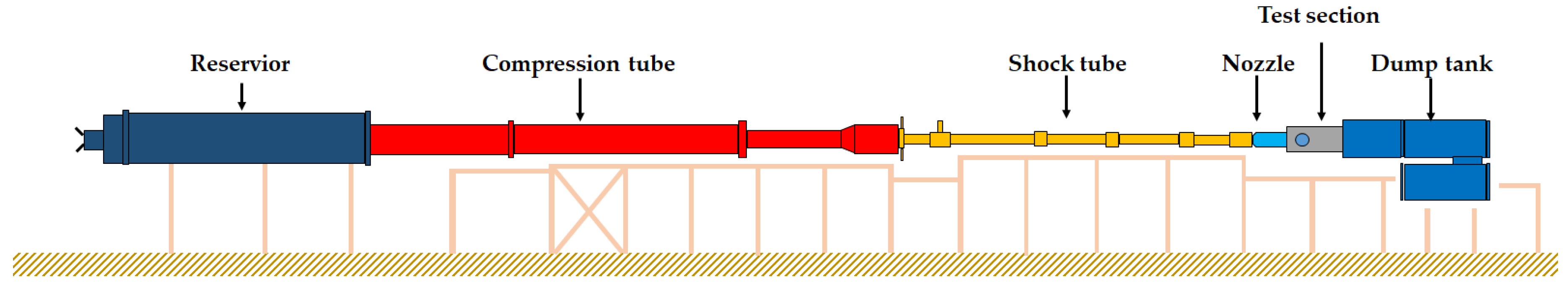For the development of a scramjet engine, in aerodynamics and combustion tests [1], ground-based test facilities, such as shock tunnels operating under high enthalpy conditions, are mainly used. For instance, several experimental and numerical studies on scramjet engines were conducted in the T4 shock tunnel, as illustrated in Figure 1 [2].

In most numerical simulations of flow in shock tunnels, the inflow conditions in the test section are determined by assuming the thermal equilibrium of the operating gas. In general, in the case of high enthalpy shock tunnels, such as T4, the flow at the exit of the nozzles entering the test section is known to be in thermochemical nonequilibrium [3,4]. The molecules in the air, which is the typical operating gas for the tests, are partially dissociated and vibrationally excited in the high-temperature reservoir of the nozzle and have little chance of intermolecular collisions in the expansion section of the nozzle, resulting in the so-called vibration freezing. In vibration freezing, the excited vibrational energy is kept constant in the downstream section of the nozzle without being relaxed with the translational and rotational modes, thereby leading to thermal nonequilibrium. Additionally, the dissociated molecules do not fully recombine at the lower temperature in the downstream section of the nozzle due to the lack of intermolecular collisions, thereby leading to chemical nonequilibrium [5]. Although the model scramjets in the test section of ground-based impulse-type facilities, such as shock tunnels, are tested using thermochemical nonequilibrium flows, the significance of incorporating the thermochemical nonequilibrium into numerical simulations for such test cases has rarely been studied.

On the other hand, the test models of a scramjet [6,7,8] are often claimed to be two-dimensional (2D) ones with finite width and wall plates at both sides, implying that 2D numerical simulations can be justifiable with the benefit of saving computational costs. However, these models designed to be nominally 2D are not completely free from the effect of sidewalls, which can only be incorporated in three-dimensional (3D) numerical simulations. Again, the significance of incorporating the sidewall effect using fully 3D numerical simulations for a nominally 2D model scramjet is not well known to the community. Therefore, when a model of a 2D scramjet, tested in a ground-based impulse facility, is simulated, and the numerical results are compared with the measured data, a situation of ambiguity remains. This observed discrepancy can be attributed to the ignorance of the thermochemical nonequilibrium states of the test flow or that of the sidewall effects in the numerical simulation.

Therefore, this study aims to analyze the significance of the modelling approach in the numerical simulation of a model scramjet, such as considering the thermochemical nonequilibrium rather than assuming equilibrium or adopting a 3D computational domain for the model rather than approximating it as a 2D domain. For this purpose, an experiment for a model scramjet [8], hereafter referred to as the Lorrain case, conducted in the T4 shock tunnel using a nominal Mach 8 nozzle with a stagnation enthalpy of 3.74 MJ/kg is adopted as a target for the present numerical simulations. The availability of detailed information on the geometry of the test model and the conditions of experiments, as well as carefully calibrated pressure measurement data, makes the Lorrain case suitable for our purpose. First, a numerical simulation of the nozzle flow is conducted with the given nozzle reservoir conditions from the experiment to define the thermochemical nonequilibrium states of the flow in the test section. Then, both 2D and 3D numerical simulations of the flow in a model scramjet are conducted for two types of inflow conditions: one with the inflow set to the thermochemical nonequilibrium states obtained from the present nozzle simulation, and the other with the inflow set to the data available from [8] where thermal equilibrium was assumed. The four simulation results are compared with the available measured data, to assess the significance of modelling approach for choosing the 2D or 3D and considering thermal equilibrium or nonequilibrium.

2. Numerical Method

The governing equations are the Navier–Stokes equations for the thermochemical nonequilibrium flows in the conservation form [9,10].

$$\frac{\partial }{\partial t}(\rho Y_s)+\stackrel{\rightharpoonup }{\nabla }·\left(\rho \stackrel{\rightharpoonup }{u}{Y}_s\right)=\stackrel{\rightharpoonup }{\nabla }·\overrightarrow{J_s}+{\dot{\omega }}_s,$$

(1)

$$\frac{\partial }{\partial t}\left(\rho \stackrel{\rightharpoonup }{u}\right)+\stackrel{\rightharpoonup }{\nabla }·\left(\rho \stackrel{\rightharpoonup }{u}\times \stackrel{\rightharpoonup }{u}\right)=\stackrel{\rightharpoonup }{\nabla }·\left[\tau \right]-\stackrel{\rightharpoonup }{\nabla }P,$$

(2)

$$\frac{\partial }{\partial t}\left(\rho E\right)+\stackrel{\rightharpoonup }{\nabla }·\left(\rho \stackrel{\rightharpoonup }{u}E\right)=\stackrel{\rightharpoonup }{\nabla }·\left({\overrightarrow{q}}_t+{\overrightarrow{q}}_v+{\displaystyle \sum }_s{\overrightarrow{J}}_s{h}_s+\stackrel{\rightharpoonup }{u}·\left[\tau \right]-P\stackrel{\rightharpoonup }{u}\right),$$

(3)

$$\frac{\partial }{\partial t}\left(\rho e_v\right)+\stackrel{\rightharpoonup }{\nabla }·\left(\rho \stackrel{\rightharpoonup }{u}{h}_v\right)=\stackrel{\rightharpoonup }{\nabla }·\left({\overrightarrow{q}}_v+{\displaystyle \sum }_s{\overrightarrow{J}}_s{h}_{s,v}\right)+{\dot{\Omega }}_v,$$

(4)

where Equation (1) is the conservation equation for the mass of species, Equation (2) is the conservation equation for momentum, Equation (3) is the conservation equation for total energy, and Equation (4) is the conservation equation for vibrational energy. $\rho$, $Y_s$, $\stackrel{\rightharpoonup }{u}$, ${\overrightarrow{J}}_s$, ${\dot{\omega }}_s$, $\left[\tau \right]$, $\overrightarrow{q}$, $h$, $e_v,$ and ${\dot{\mathsf{\Omega }}}_v$ represent the density, mass fraction of species, velocity, mass diffusion flux of species, rate of production of species, viscous stress tensor, conduction heat flux, enthalpy per unit mass species, internal energy, and source term which represents the coupling between the vibrational and translational-rotational energy, respectively [9,10]. The subscripts s, t, and v indicate species, translational-rotational energy mode, and vibrational energy mode, respectively [9]. To solve the above equations, mass diffusion flux, viscous stress tensor, and conduction heat flux must be modeled. The conduction heat flux is modeled by Fourier’s law of heat conduction and the mass diffusion flux is modeled by Fick’s law as Equations (5)–(7) [10];

$${\overrightarrow{J}}_s=\rho D_s\stackrel{\rightharpoonup }{\nabla }{Y}_s,$$

(5)

$$\left[\tau \right]=\mu \left(\stackrel{\rightharpoonup }{\nabla }\stackrel{\rightharpoonup }{u}+{(\stackrel{\rightharpoonup }{\nabla }\stackrel{\rightharpoonup }{u})}^T\right)-\frac{3}{2}\mu (\stackrel{\rightharpoonup }{\nabla }·\stackrel{\rightharpoonup }{u})\left[\mathrm{I}\right],$$

(6)

$${\overrightarrow{q}}_k={\lambda }_k\stackrel{\rightharpoonup }{\nabla }{T}_k, k=t or v,$$

(7)

where $\mu$, $D_s$, $\left[\mathrm{I}\right]$, $T_k$, and ${\lambda }_k$ represent gas viscosity coefficient, diffusion coefficient of species, identity matrix, temperature, and thermal conductivity coefficient, respectively [10].

The two-temperature model is the most fundamental model available in modelling thermal nonequilibrium as it assumes a single temperature for the translational-rotational mode and another single temperature for the vibrational electronic excitation for all the molecules [11,12]. As this study focuses on the difference between the thermal equilibrium and thermal nonequilibrium, the primitive two-temperature model is adopted rather than more complicated multitemperature models. The translational and vibrational relaxation rates are given by the Landau–Teller equation with the modified Millikan–White relaxation time model [13]. There are options at different levels of fidelity and complexity in describing the nonequilibrium energies to model hypersonic flows. One of the immediate ways of increasing the complexity of the modelling is to treat the vibrational temperature of ${\mathrm{N}}_2, {\mathrm{O}}_2$, and NO independently. To do so, the vibrational–vibrational energy exchanges among the three molecules need to be incorporated. As the energy transfer rates are not known accurately, this increase in complexity does not necessarily increase the fidelity of the model. Moreover, the vibrational coupling between the three molecules is known to be strong. In the study [14] where three vibrational temperature and electron temperature were calculated independently, the results showed that these four temperatures were nearly identical, which justifies the validity of the two-temperature model. On the other hand, often the associative ionization to produce ${\mathrm{NO}}^{+}$ and subsequent electron-impact ionization might be considered in the modelling. However, the ionization of air species is only activated at the very high temperature corresponding to the post-shock condition of the inflow velocities over 10 km/s. In general, for the range of the temperature below 4000 K of the present study at the velocity of approximately 2.5 km/s, ionization can be safely ignored. Although the two-temperature model has its own limitation [15], the flow regime of the present study falls into the area where the two-temperature model is considered to be acceptable.

To solve the thermochemical nonequilibrium Navier–Stokes equations, a two-temperature open-source solver for hypersonic reacting flows, called hy2Foam [9], is adopted. hy2Foam is a fusion of additional physical models to incorporate thermochemical nonequilibrium with the existing solver called rhoCentralFoam, developed for compressible flows and based on the OpenFOAM framework [16]. The thermochemical nonequilibrium modelling of the solver was validated for several cases ranging from zero-dimensional chemical kinetics to multidimensional hypersonic flows [9,17,18,19], and the underlying numerics of the solver was also validated for the hypersonic cases relevant to the present study [20,21,22].

In the present study, the chemical mechanism [11], which contains five reactions for the five neutral air species, is employed. The reaction rate coefficients for the air chemistry are summarized in

Table 1. Reaction rate coefficients [11].

Reaction	${\mathit{k}}_{\mathit{f}}=\mathit{A}{\mathit{T}}_{\mathit{a}\mathit{v}\mathit{e}}^{\mathit{\beta }}\mathbf{exp}(-{\mathit{T}}_{\mathit{r}}/{\mathit{T}}_{\mathit{a}\mathit{v}\mathit{e}})$
	$\mathit{M}$	$\mathit{A}$1	$\mathit{\beta }$	${\mathit{T}}_{\mathit{r}}$	${\mathit{T}}_{\mathit{a}\mathit{v}\mathit{e}}$
$O_2+M\to 2O+M$	$O$	$1.0\times {10}^{19}$	−1.5	59,500	$\sqrt{T_t{T}_v}$
	$N$	$1.0\times {10}^{19}$
	$NO$	$2.0\times {10}^{18}$
	$N_2$	$2.0\times {10}^{18}$
	$O_2$	$2.0\times {10}^{18}$
$N_2+M\to 2N+M$	$O$	$3.0\times {10}^{19}$	−1.6	113,220	$\sqrt{T_t{T}_v}$
	$N$	$3.0\times {10}^{19}$
	$NO$	$7.0\times {10}^{18}$
	$N_2$	$7.0\times {10}^{18}$
	$O_2$	$7.0\times {10}^{18}$
$NO+M\to N+O+M$	$O$	$1.1\times {10}^{14}$	0	75,500	$\sqrt{T_t{T}_v}$
	$N$	$1.1\times {10}^{14}$
	$NO$	$5.0\times {10}^{12}$
	$N_2$	$5.0\times {10}^{12}$
	$O_2$	$5.0\times {10}^{12}$
$N_2+O\to NO+N$	-	$6.4\times {10}^{14}$	−1.0	38,400	$T_t$
$NO+O\to N+O_2$	-	$8.4\times {10}^9$	0	19,450	$T_t$

¹$A$ is in $\mathrm{L}\mathrm{m}\mathrm{o}{\mathrm{l}}^{-1}{\mathrm{s}}^{-1}$.

. The equilibrium constants [23] are calculated as shown in Equation (8):

$$K_{eq}=exp\left(A{Z}^5+B{Z}^4+C{Z}^3+D{Z}^2+EZ+F\right)$$

(8)

where $Z=\ln \left({10}^4/T\right)$. The backward reaction rate coefficients are obtained from the forward reaction rates and the equilibrium constants. Park’s dissociation model [13], which defines the average vibrational energy transferred in dissociation to be 30% of the dissociation energy, is adopted.

The molecular viscosity of the species is obtained using Blottner’s viscosity model [24] and the thermal conductivity of the species is obtained by Eucken’s formula [25]. The transport properties for the mixture are given by Wilke’s mixing rule [26] and the diffusion fluxes are given by Fick’s law [27,28].

The solver adopts an implicit finite volume method provided by the OpenFOAM framework. The convective fluxes are discretized using the second order Kurganov–Tadmor central-upwind scheme [29] with van Leer limiter. The pseudo-transient scheme for accelerating a solution to the steady state using local time stepping (LTS) is adopted. An MPI parallel computing based on domain decomposition is utilized on multiple Xeon CPU cores. A simulation for one flow-through time takes 125.4 core-hours for 2D-equilibrium, 138.6 core-hours for 2D-nonequilibrium, 9922 core-hours for 3D-equilibrium, and 11,132 core-hours for 3D-nonequilibrium simulations.

3. Test Conditions

The model scramjet experiment of Lorrain was conducted in the T4 shock tunnel at the University of Queensland. The axisymmetric, contoured nominal Mach 8 nozzle of the T4 shock tunnel was designed by Craddock [3]. The enthalpy and pressure of the nozzle reservoir were 3.74 MJ/kg and 44.2 MPa, respectively [8]. The test gas was air. The Mach number of the nozzle exit flow was 7.53 [8]. The model scramjet was based on the nominally 2D scramjet configuration presented by Boyce et al. [30]. By using the properties of the nozzle exit flow of the T4 shock tunnel as the inflow conditions of the model scramjet, the experiment was conducted with fuel injection and without fuel injection; however, in the present study, only the experiment without fuel injection is considered.

4. Computational Setup

4.1. T4 Shock Tunnel Nozzle Flow

In the present study, the wedge-shaped finite-volume mesh of the nozzle, as depicted in Figure 2, was used to calculate the axisymmetric nozzle flow. The nozzle had a diameter of 16.4 mm at the throat and 0.27 m at the exit. The length of the expansion section was 1.11 m and the wedge angle was 4°. The number of mesh cells was 150 × 60. The nozzle reservoir conditions were obtained from the experiment of Lorrain: a stagnation pressure of 44.2 MPa and a stagnation enthalpy of 3.74 MJ/kg. Additionally, a non-slip wall condition was applied. The numerical simulation was conducted by using the thermochemical nonequilibrium assumption, and the obtained flow properties were pressure of 1877.99 Pa, Mach number of 8.42, translational temperature of 260.68 K, vibrational temperature of 640.32 K, and density of 0.02471 $\mathrm{kg}/{\mathrm{m}}^3$.

Figure 3 illustrates the distributions of the temperature of the calculated nozzle flow along the center line of the nozzle. The temperature at the nozzle reservoir was as high as 3400 K and decreased as the gas expanded beyond the nozzle throat. Near the point where the center line was approximately 0.5 m, the temperature was separated into translational temperature and vibrational temperature. At the freezing point, the vibrational temperature stayed nearly constant, becoming 640.32 K at the nozzle exit. On the other hand, the translational temperature continued to decrease, becoming 260.68 K at the nozzle exit.

4.2. Setup for Model Scramjet

The model scramjet of Lorrain comprises two ramps, a combustor, and a nozzle. The configuration of the model scramjet is asymmetric about the x-z plane and symmetric about the x-y plane, as depicted in Figure 4. The flow turning angles were 9.7° and 3° for the first and second ramps of the top surface, respectively. For the bottom surface, the flow turning angles were 9° and 3° for the first and second ramps, respectively. The length of the combustor was 382.6 mm and the height of the combustor was 26 mm. The width of the model scramjet was 75 mm. The 5 mm of the inflow domain was added in front of the inlet to implement the inflow in the test section effectively. The number of mesh cells was 147,312 for the 2D computational domain and 7,365,600 for the 3D computational domain. For the 3D computational domain, only the half-width of the model was considered, utilizing the symmetric condition at the central plane in the z-direction, to reduce the computational cost. The number of cells used in the present 2D simulation was larger than the baseline cell number used in [8], which was confirmed to be adequate. To ensure the refined mesh near the wall, without adopting any wall function, y+ was selected to be smaller than unity. As a result, the distance from the first grid of each wall was fixed at 5 µm.

The inflow conditions for the computational domain of the model scramjet are described by the flow properties at the T4 nozzle exit, which are available from two sources: one is the thermochemical nonequilibrium states obtained from the simulation described in Section 4.1, and the other is the data from [8], which was obtained using the thermal equilibrium and chemical nonequilibrium assumptions. These two sets of inflow conditions are summarized in

Table 2. Flow properties at the nozzle, used for inflow conditions of the model scramjet.

	Present CFD	Lorrain [8]
Mach	8.42	7.53
P (Pa)	1877.99	3750
${\mathit{T}}_{\mathit{t}}$(K)	260.68	315.4
${\mathit{T}}_{\mathit{v}}$(K)	640.32	315.4
U (m/s)	2734.33	2684
$\mathsf{\rho }$$(kg/m^3$)	0.02471	0.00412
${\mathit{Y}}_{{\mathit{N}}_2}$	0.760186	0.7456
${\mathit{Y}}_{{\mathit{O}}_2}$	0.223044	0.2063
${\mathit{Y}}_{\mathit{N}\mathit{O}}$	0.01677	0.04789
${\mathit{Y}}_{\mathit{N}}$	$0$	0
${\mathit{Y}}_{\mathit{O}}$	$5.7558\times {10}^{-8}$	0.00016

. For the preceding section before the leading edge of the ramp, a slip wall condition was applied. For all the walls, a non-slip and an iso-thermal condition at 300 K were applied. To describe turbulence, the RANS k-ω SST model was used.

4.3. Grid Independence and Validation Study

A grid independence test was carried out for the two-dimensional numerical simulations of the flow in the model scramjet, with the thermochemical nonequilibrium inflow conditions, by using four sets of meshes. Figure 5 compares the distributions of the normalized pressure along the bottom wall of the model scramjet by using 46,872; 97,464; 147,312; and 220,596 cells, respectively. The solution using the coarsest grid fails to capture the first reflection of the incident shock wave and the subsequent structure of the shock train. Except for the solution with the coarsest grid, the solutions of the rest of the grids are in good agreement showing convergence along with the increase of grid resolution. The solutions using 147,312 cells and 220,596 cells are practically indistinguishable, which confirms that the numerical solution of the present study with 147,312 cells is grid independent.

To validate the numerical methods of the present study using hy2Foam, two types of validation cases were selected: (1) an adiabatic reactor of nitrogen molecules for the relaxation of nonequilibrium temperatures for vibrational heating/cooling towards higher/lower translational-rotational temperature and (2) a hypersonic flow of Mach 11.3 over a blunted cone with a spherical nose of 6.35 radius and a half-cone angle of 25 degrees.

The numerical solutions of the present study for the zero-dimensional adiabatic reactor initially in temperature nonequilibrium undergoing relaxation between temperatures are shown in Figure 6 with the solutions of hy2Foam available from [17], the solutions of LeMANS (The Michigan Aerothermodynamic Navier–Stokes solver) [31], and the solutions of MONACO, a direct simulation of Monte-Carlo code [31]. For both vibrational heating and cooling, the temperature relaxation processes obtained by the present simulations are in good agreement with the data available from the literature.

The present solution of a two-dimensional axisymmetric numerical simulation for the Mach 11.3 hypersonic flow over a blunted cone is shown in Figure 7 using the pressure coefficient along the axial distance from the stagnation point, together with other numerical solutions [9,32] and experimental data [33]. The numerical solutions are consistent with each other, whereas all the numerical solutions show minor deviations from the experimental data.

Through the above validation tests, the present numerical methods are shown to be valid to be applied for a multidimensional nonequilibrium hypersonic flows with the capability of accurate reproduction of temperature relaxation process and flow structure behind the hypersonic shock wave.

5. Results and Discussion

Both 2D and 3D numerical simulations of the flow in a model scramjet were conducted for two different inflow conditions summarized in Table 2. With the thermochemical nonequilibrium inflow conditions, the numerical simulations for the model scramjet were conducted using the thermochemical nonequilibrium assumption as well. A thermal equilibrium assumption was imposed for the simulations using the inflow conditions of thermal equilibrium. As a result, four cases were investigated and compared with the available measured data to assess the significance of the modelling approach for choosing between 2D or 3D, and thermal equilibrium or nonequilibrium. For brevity, the four cases are denoted as 2D-equilibrium, 2D-nonequilibrium, 3D-equilibrium, and 3D-nonequilibrium, respectively.

Figure 8 depicts the numerical schlieren images extracted from the results of the four numerical simulations, where the directions of the flows are from left to right. The oblique shocks formed from the first and second ramps of the intake interact with the expansion wave, thereby producing a single shock train. Due to the shock reflections on the combustor wall, three pressure peaks are observed in the combustor section. The interaction of the incident shock into the combustor section and the boundary surfaces of the combustor section forms a separation bubble at the intersecting region due to a strong adverse pressure gradient (see Figure 9b for details). As the geometry of the model is slightly asymmetric between the upper surface and lower surface of the intake (see Figure 4), the shock interactions and reflections in the combustor section and its downstream remain in slight asymmetry. Consequently, while the first crossing point of the reflected shock waves from the upper and lower combustor walls is near the vertical center of the combustor, the second and third crossing points are closer to the lower combustor wall and upper combustor wall, respectively. It can be seen that the shock train structure is well resolved without excessive numerical dissipation in the present simulations.

Figure 9 depicts the distributions of the pressure of the 3D-nonequilibrium case for the x-y plane along z = 0. As depicted in Figure 9b, the flow separation regions appear at the first reflected shock wave on both the combustor walls of the model scramjet. This is attributed to the strong adverse gradient of pressure along these surfaces during the shock-boundary layer interaction.

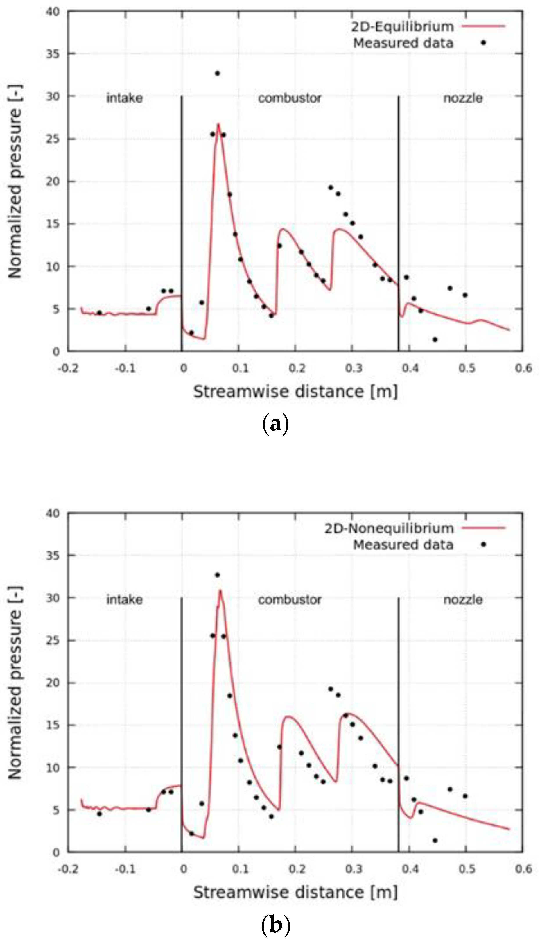
For a fair comparison between the nonequilibrium and equilibrium cases, the discrepancy of the pressure in the inflow conditions of each assumption needs to be addressed. Therefore, a normalized pressure, which is to be calculated using the following equation, is used:

$$P_{norm}=\frac{P_{mean}}{P_{\infty }}$$

(9)

where $P_{\infty }$ is the pressure of the inflow condition.

As presented in Table 2, $P_{\infty }=3750\mathrm{Pa}$ for the equilibrium cases and $P_{\infty }=1877.99\mathrm{Pa}$ for the nonequilibrium cases. In Figure 10, the normalized pressure data measured along the centerline of the bottom wall of the model from the experiment of [8] is compared with those from the present numerical simulations. In subfigures of Figure 10, the stations at the beginning and end of the combustor section are denoted as two vertical lines at x = 0 and x = 0.3826 m. Regarding the axial locations of the pressure peaks, the numerical solutions using the thermal equilibrium assumption with the inflow conditions of thermal equilibrium are in good agreement with the measured data, whereas those using the thermal nonequilibrium assumption with the inflow conditions of thermal nonequilibrium exhibit spatial delays in the downstream, past the first shock reflection point. However, regarding the strength of the pressure peaks due to shock interactions and reflections, the two nonequilibrium cases show better agreement with the measured data than the equilibrium cases. Between the 2D and 3D simulation results, the pressure peak values obtained from the 3D simulations are in better agreement with respect to the measured data than those from the 2D simulations, regardless of the thermal equilibrium or nonequilibrium. This can be explained by the fact that the compression effect along the side walls can only be incorporated in the 3D simulations; hence, the pressure values from the 3D simulations tend to be greater than those from the 2D simulations.

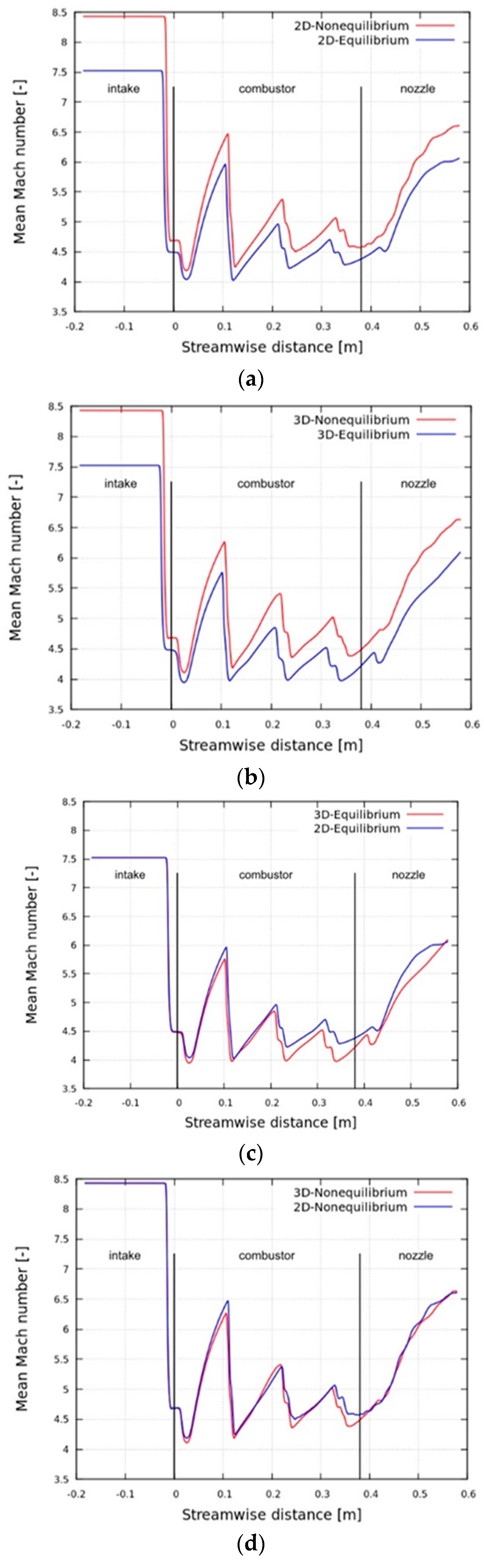
Figure 11 illustrates the differences in the values of Mach number along the centerline between the 2D and 3D cases, and between the equilibrium and nonequilibrium cases. Figure 11a,b shows that the nonequilibrium cases exhibit higher values of Mach number than the equilibrium cases throughout the model scramjet; however, regarding the shock wave positions, the nonequilibrium cases are shifted backward in comparison with the equilibrium cases. These tendencies are consistent with the relations between normalized pressure and the four simulation cases, as depicted in Figure 10. It can be interpreted that higher the Mach number, the smaller the angle of the oblique shock wave, and the smaller angled oblique shock wave causes the reflected shock waves to be shifted backward in position. From Figure 11c,d, the 2D cases exhibit slightly higher values of Mach number than the 3D cases at the first reflected shock; however, in general, there is little difference between them.

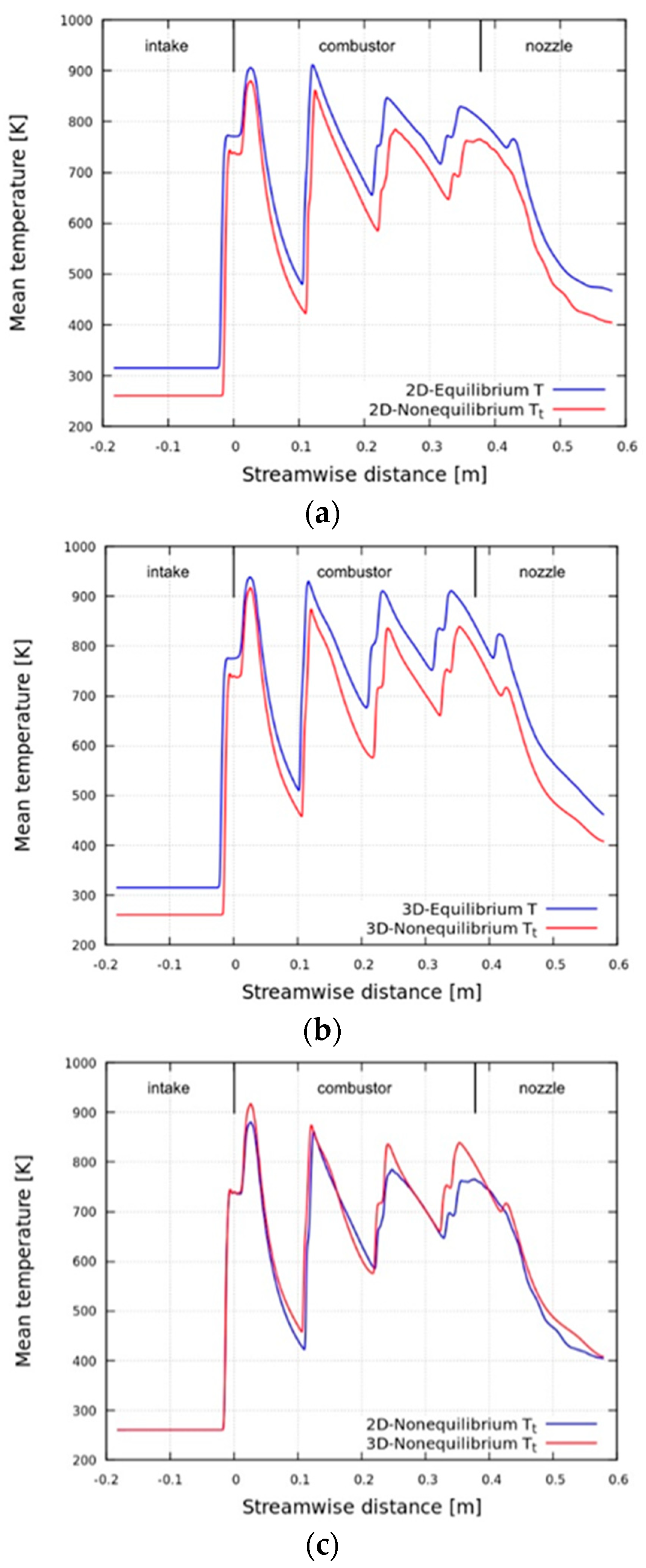
Figure 12 exhibits the distributions of temperature along the centerline of the model scramjet configuration. When the values of the temperature of the equilibrium cases are compared with the values of the translational-rotational temperature of the nonequilibrium cases for the 2D cases (Figure 12a) and 3D cases (Figure 12b), respectively, the discrepancy in the translational-rotational temperatures given from the inflow condition persists throughout the model scramjet. However, the discrepancy is reduced in the rising phase (post-shock region) and increased in the decaying phase (expanding region before the following shock reflections), which is physically intuitive as the collision frequency increases in the post-shock region and decreases in the expanding region, thereby leading the nonequilibrium translational-rotational temperature toward equilibrium and away from equilibrium, respectively. The nonequilibrium temperatures are compared between the 2D cases and 3D cases for the translational-rotational temperatures (Figure 12c) and for vibrational temperature (Figure 12d). Both the translational-rotational temperature and vibrational temperature are higher for the 3D case than for the 2D case, which is again postulated to be affected by the compression due to the presence of sidewalls. The compression effect is more pronounced in the downstream of the combustor section, which is plausible as the displacement thickness due to the boundary layer from the sidewalls increases along the combustor section. Finally, Figure 12e shows the distributions of the two temperatures for the 3D nonequilibrium case. The translational-rotational temperature has sharp variations in the combustor section in accordance with the structure of the shock train, whereas the vibrational temperature has only small variations. This implies that the strong thermal nonequilibrium originating from the nozzle of the test facility is maintained throughout the model scramjet despite the potential collisions between molecules over multiple reflections and interactions of oblique shocks through the shock train in the combustor section. The insensitivity of vibrational temperature to the variation of translational temperature is attributed to the relatively large vibrational relaxation time in comparison with the flow residence time between the shock interactions in the shock train. For example, the flow residence time between the first shock interaction at approximately x = 0.1 m and the second shock interaction at approximately x = 0.2 m is approximately 40 $\mathsf{\mu }\mathrm{s}$. However, the vibrational relaxation time according to the Millikan and White model, at its minimum at the post-shock region is approximately 20$\mathsf{\mu }\mathrm{s}$, and then increases quickly up to approximately 850 $\mathsf{\mu }\mathrm{s}$ along with the flow expansion. The vibrational relaxation time is inversely proportional to pressure (linear) and temperature (nonlinear), while the pressure and temperature drops to 0.06 atm and 440 K near x = 0.2 m. The increase in the temperature and pressure at post-shock is across a very short length scale, whereas the decrease of those takes place for the rest of the region between x = 0.1 and 0.2 m along with the flow expansion. Therefore, the vibrational temperature follows the translational-rotational temperature at a relatively low relaxation rate in the combustor section. In the nozzle of the model scramjet, the translational temperature continues to decrease, while the vibrational temperature stays nearly constant, again demonstrating vibrational freezing. This tendency is consistent with the distribution of temperature in the nozzle flow in the T4 shock tunnel depicted in Figure 3.

6. Conclusions

The ground tests using model scramjet engines are typically conducted in hypervelocity facilities where the nozzle flow entering the test section is in the thermochemical nonequilibrium state. However, in general, the inflow conditions for the model scramjets in such test sections are often obtained under the thermal equilibrium assumption, resulting in a lower Mach number than the actual Mach number in the test section because the translational temperature is predicted to be higher than the actual translational temperature, due to the thermal equilibrium with vibrational temperature. The significance of this approximation of the incoming flow into the test section in the analysis of the flow through model scramjets has not been investigated thus far. Moreover, when a model scramjet is designed nominally to be 2D, it can never be completely free from the effect of the sidewalls. Considering these concerns, the present study attempted to assess the significance of the choice of the modelling approach in the numerical simulations of a model scramjet engine. Both 2D and 3D numerical simulations were conducted by using two inflow conditions: one was the thermochemical nonequilibrium states obtained from the simulation of nozzle exit flow, and the other was the thermal equilibrium states available from the team that originally tested the model scramjet in the T4 shock tunnel. The four results were compared with the measured data available to assess the significance of the modelling approach to choose between 2D or 3D, and thermal equilibrium or nonequilibrium. Increasing the fidelity of the simulation by modelling the domain from 2D to 3D, and treating the flow from thermal equilibrium to nonequilibrium, the corresponding numerical solutions are improved in general, in terms of the agreement with the available experimentally measured data. It is notable that the flow is in the thermal nonequilibrium state not only in the nozzle of the test facility but also throughout the flow passage over the model scramjet engine studied in the present study. The 3D modelling turns out to be important as it can incorporate the compression effect of the sidewalls.

References

1. Anderson, J.D., Jr. Hypersonic and High-Temperature Gas Dynamics, 2nd ed.; American Institute of Aeronautics and Astronautics: Reston, VA, USA, 2006. [Google Scholar]
2. T4-Free-Piston Driven Shock Tunnel. Available online: http://hypersonics.mechmining.uq.edu.au/t4 (accessed on 29 January 2020).
3. Craddock, C.S. Design of the Axisymmetric HyShot Nozzle for T4; Research Report 2/00; Department of Mechanical Engineering, University of Queensland: Brisbane, Australia, 2000. [Google Scholar]
4. Furudate, M.; Lee, B.J.; Jeung, I.S. Computation of Hyshot Scramjet Flows in the T4 Experiments. In Proceedings of the AIAA/CIRA 13th International Space Planes and Hypersonics Systems and Technologies Conference, Capua, Italy, 16–20 May 2005. AIAA Paper 2005–3353. [Google Scholar]
5. Park, C. Nonequilibrium Hypersonic Aerothermodynamics; John Wiley & Sons, Inc.: New York, NY, USA, 1989. [Google Scholar]
6. Paull, A.; Frost, M.; Alesi, H. HyShot-T4 Supersonic Combustion Experiments; Report NAG–1–2113; University of Queensland: Brisbane, Australia, 2000. [Google Scholar]
7. Tetsuji, S.; Katsuhiro, I.; Kazuo, S.; Tomoyuki, K. Mach 8 Ground Tests of the Hypermixer Scramjet for HyShot-IV Flight Experiment. In Proceedings of the 14th AIAA/AHI Space Planes and Hypersonic Systems and Technologies Conference, Canberra, Australia, 6–9 November 2006. AIAA Paper 2006–8062. [Google Scholar]
8. Lorrain, P. Flow Structure/Chemistry Coupling in the Ignition Process in Shock-Induced-Combustion Scramjets. Ph.D. Thesis, School of Mechanical and Mining Engineering, University of Queensland, Brisbane, Australia, 2014. [Google Scholar]
9. Casseau, V.; Espinoza, D.E.R.; Scanlon, T.J.; Brown, R.E. A two-temperature open-source CFD model for hypersonic reacting flows, part two: Multi-dimensional analysis. Aerospace 2016, 3, 45. [Google Scholar] [CrossRef] [Green Version]
10. Loureiro, D.D. High-Temperature Modeling of Transport Properties in Hypersonic Flows. Ph.D. Thesis, Instituto Superior Técnico, Lisbon, Portugal, 2015. [Google Scholar]
11. Park, C. Review of chemical-kinetic problems of future NASA missions. I-Earth entries. J. Thermophys. Heat Trans. 1993, 7, 385–398. [Google Scholar] [CrossRef]
12. Park, C.; Howe, J.T.; Jaffe, R.L.; Candler, G.V. Review of chemical-kinetic problems of future NASA missions. II-Mars entries. J. Thermophys. Heat Trans. 1994, 8, 9–23. [Google Scholar] [CrossRef]
13. Sharma, S.P.; Huo, W.M.; Park, C. Rate parameters for coupled vibration-dissociation in a generalized SSH approximation. J. Thermophys. Heat Trans. 1992, 6, 9–21. [Google Scholar] [CrossRef]
14. Candler, G.V.; MacCormack, R.W. The Computation of Hypersonic Ionized Flows in Chemical and Thermal Nonequilibrium. In Proceedings of the 26th Aerospace Sciences Meeting, Reno, NE, USA, 11–14 January 1988. AIAA Paper 1988–0511. [Google Scholar]
15. Park, C. The Limits of Two-Temperature Kinetic Model in Air. In Proceedings of the 48th AIAA Aerospace Sciences Meeting Including the New Horizons Forum and Aerospace Exposition, Orlando, FL, USA, 4–7 January 2010. AIAA Paper 2010–0911. [Google Scholar]
16. Weller, H.G.; Tabor, G.; Jasak, H.; Fureby, C. A tensorial approach to computational continuum mechanics using object-oriented techniques. Comput. Phys. 1998, 12, 620–631. [Google Scholar] [CrossRef]
17. Casseau, V.; Palharini, R.C.; Scanlon, T.J.; Brown, R.E. A two-temperature open-source CFD model for hypersonic reacting flows, part one: Zero-dimensional analysis. Aerospace 2016, 3, 34. [Google Scholar] [CrossRef] [Green Version]
18. Casseau, V.; Scanlon, T.J.; Brown, R.E. Development of a Two-Temperature Open-Source CFD Model for Hypersonic Reacting Flows. In Proceedings of the 20th AIAA International Space Planes and Hypersonic Systems and Technologies Conference, Glasgow, UK, 6–9 July 2015. AIAA Paper 2015–3637. [Google Scholar]
19. Hoste, J.J.O.; Casseau, V.; Fossati, M.; Taylor, I.J.; Gollan, R. Numerical Modeling and Simulation of Supersonic Flows in Propulsion Systems by Open-Source Solvers. In Proceedings of the 21st AIAA International Space Planes and Hypersonics Technologies Conference, Xiamen, China, 6–9 March 2017. AIAA Paper 2017–2411. [Google Scholar]
20. Soni, R.K.; Arya, N.; De, A. Assessment of RANS Based Models in a Supersonic Flow. In Proceedings of the 12th International Conference of Numerical Analysis And Applied Mathematics ICNAAM 2014, Rhodes Island, Greece, 22–28 September 2014; Volume 1648, p. 030039. [Google Scholar]
21. Hinman, W.S.; Johansen, C.T. Rapid prediction of hypersonic blunt body flows for parametric design studies. Aerosp. Sci. Technol. 2016, 58, 48–59. [Google Scholar] [CrossRef]
22. Teh, E.J.; Johansen, C.T. Effect of particle momentum transfer on an oblique-shock-wave/laminar-boundary-layer interaction. Acta Astronaut. 2016, 128, 431–439. [Google Scholar] [CrossRef]
23. Park, C.; Jaffe, R.L.; Partridge, H. Chemical-kinetic parameters of hyperbolic earth entry. J. Thermophys. Heat Trans. 2001, 15, 76–90. [Google Scholar] [CrossRef]
24. Blottner, F.G.; Johnson, M.; Ellis, M. Chemically Reacting Viscous Flow Program for Multi-Component Gas Mixtures; Report SC-RR-70-754; Sandia Laboratories: Albuquerque, NM, USA, 1971. [Google Scholar]
25. Kruger, C.H.; Vincenti, W.G. Introduction to Physical Gas Dynamics; John Wiley & Sons, Inc.: New York, NY, USA, 1965. [Google Scholar]
26. Wilke, C.R. A viscosity equation for gas mixtures. J. Chem. Phys. 1950, 18, 517–519. [Google Scholar] [CrossRef]
27. Liu, I.S. On Fourier’s law of heat conduction. Continuum Mech. Therm. 1990, 2, 301–305. [Google Scholar] [CrossRef]
28. Van Milligen, B.P.; Bons, P.D.; Carreras, B.A.; Sanchez, R. On the applicability of Fick’s law to diffusion in inhomogeneous systems. Eur. J. Phys. 2005, 26, 913. [Google Scholar] [CrossRef]
29. Kurganov, A.; Tadmor, E. New high-resolution central schemes for nonlinear conservation laws and convection–diffusion equations. J. Comput. Phys. 2000, 160, 241–282. [Google Scholar] [CrossRef] [Green Version]
30. Boyce, R.R.; Schloegel, F.; McIntyre, T.J.; Tirtey, S.C. Pressure-Scaling of Inlet-Injection Radical-Farming Scramjets. In Proceedings of the 20th International Symposium on Airbreathing Engines, Gothenburg, Sweden, 12–16 September 2011; pp. 1322–1332. [Google Scholar]
31. Boyd, I.D.; Josyula, E. State resolved vibrational relaxation modeling for strongly nonequilibrium flows. Phys. Fluids 2011, 23, 057101. [Google Scholar] [CrossRef] [Green Version]
32. Wang, W.L.; Boyd, I. Hybrid DSMC-CFD Simulations of Hypersonic Flow over Sharp and Blunted Bodies. In Proceedings of the 36th AIAA Thermophysics Conference, Orlando, FL, USA, 23–26 June 2003. AIAA Paper 2003–3644. [Google Scholar]
33. Holden, M.S. Experimental Database from CUBRC Studies in Hypersonic Laminar and Turbulent Interacting Flows Including Flowfield Chemistry; RTO Code Validation of DSMC and Navier–Stokes Code Validation Studies CUBRC Report; Calspan-University at Buffalo Research Center: Buffalo, NY, USA, 2000. [Google Scholar]
Figure 1. Schematic of the T4 shock tunnel [2].
Energies 13 00606 g001
Figure 2. Computational domain of the nozzle of the T4 shock tunnel.
Energies 13 00606 g002
Figure 3. Distributions of temperature along the center line of the nozzle flow.
Energies 13 00606 g003
Figure 4. Computational domain of the model scramjet of Lorrain.
Energies 13 00606 g004
Figure 5. Grid independence for normalized pressure distributions along the bottom wall.
Energies 13 00606 g005
Figure 6. Vibrational translational relaxation towards equilibrium of a nitrogen heat bath: (a) vibrational heating; (b) vibrational cooling [17].
Energies 13 00606 g006
Figure 7. Distributions of pressure coefficient along the axial distance from stagnation point [9].
Energies 13 00606 g007
Figure 8. Numerical schlieren images for four simulation cases: (a) 2D-equilibrium case; (b) 2D-nonequilibrium case; (c) 3D-equilibrium case; (d) 3D-nonequilibrium case.
Energies 13 00606 g008
Figure 9. Pressure contours of (a) 3D-nonequilibrium case; (b) 3D-nonequilibrium case, zoomed in for the first shock reflection points for the x-y plane along z = 0.
Energies 13 00606 g009aEnergies 13 00606 g009b
Figure 10. Distributions of normalized pressure along the bottom wall: (a) 2D-equilibrium case; (b) 2D-nonequilibrium case; (c) 3D-equilibrium case; (d) 3D-nonequilibrium case.
Energies 13 00606 g010aEnergies 13 00606 g010b
Figure 11. Distributions of Mach number along the centerline (y = 0, z = 0): (a) 2D cases; (b) 3D cases; (c) equilibrium cases; (d) nonequilibrium cases.
Energies 13 00606 g011
Figure 12. Distributions of temperature along the centerline (y = 0, z = 0): (a) temperature of the equilibrium case and translational-rotational temperature of the nonequilibrium case for the 2D cases; (b) temperature of the equilibrium case and translational-rotational temperature of the nonequilibrium case for the 3D cases; (c) translational-rotational temperature of the nonequilibrium cases; (d) vibrational temperature of the nonequilibrium cases; (e) translational-rotational and vibrational temperature of the 3D-nonequilibrium case.
Energies 13 00606 g012aEnergies 13 00606 g012b