Optimization of Isolated Hybrid Microgrids with Renewable Energy Based on Different Battery Models and Technologies


1
Electronic Engineering Department, San Buenaventura University, Carrera 8H # 172-20 Bogota, Colombia
2
Electrical Engineering Department, University of Zaragoza, Calle María de Luna 3, 50018 Zaragoza, Spain
*
Author to whom correspondence should be addressed.
Energies 2020, 13(3), 581; https://doi.org/10.3390/en13030581
Submission received: 27 December 2019
/
Revised: 20 January 2020
/
Accepted: 22 January 2020
/
Published: 26 January 2020
Abstract
:Energy supply in remote areas (mainly in developing countries such as Colombia) has become a challenge. Hybrid microgrids are local and reliable sources of energy for these areas where access to the power grid is generally limited or unavailable. These systems generally include a diesel generator, solar modules, wind turbines, and storage devices such as batteries. Battery life estimation is an essential factor in the optimization of a hybrid microgrid since it determines the system’s final costs, including future battery replacements. This article presents a comparison of different technologies and battery models in a hybrid microgrid. The optimization is achieved using the iHOGA software, based on data from a real microgrid in Colombia. The simulation results allowed the comparison of prediction models for lifespan calculation for both lead–acid and lithium batteries in a hybrid microgrid, showing that the most accurate models are more realistic in predicting battery life by closely estimating real lifespans that are shorter, unlike other simplified methods that obtain much longer and unrealistic lifetimes.
1. Introduction
Global warming and the increase of greenhouse gases caused by fossil-fuel-based energy generation have resulted in worldwide concern about future energy supply [1]. These inconveniences have become an opportunity for the use of renewable energy such as solar, wind, tidal, geothermal, and biomass, among others. In 2018, approximately 15% of the total energy consumed worldwide was of renewable origin, and it is estimated that by 2050 this percentage may reach 28% [2]. In terms of electrical energy generated, renewable sources generated 28% of the total worldwide energy in 2018, and it is estimated that they could produce 49% by 2050 [2], reducing fossil fuel dependence and mitigating the effects caused by climate change. However, one drawback of renewable sources is their unpredictable nature and intermittency. To overcome this drawback, an attractive solution is to combine two or more energy sources in a hybrid system and include energy storage [3]. For example, photovoltaic power generation can be used during the day and wind power generation (which usually generates more energy) can be used at night, so the two sources of energy complement each other [4,5]. Furthermore, the different energy sources can be managed as a microgrid, which can solve reliability problems and provide an environmentally friendly solution [6]. In addition, increasing renewable energies can cause problems for quality; therefore, it is necessary to have a flexible and intelligent electrical network. One of the fundamental aspects to increase the electrical grid’s flexibility is the use of storage systems that allow compensation for the variability of renewable energy sources. Conversely, electricity grids are designed considering energy sources that do not present variability, which happens with renewables, so electricity grids must have enough back-up capacity. Storage capacity is essential, thus making it possible to increase renewable generation while avoiding the possible problems that could be caused by its variability [3].
Hybrid microgrids are a new solution in remote areas that are difficult to access or that do not have access to conventional power grids [7]. In hybrid microgrids based on renewable energy, one of the main elements that support the energy supply due to the variable intermittency such as radiation or wind, as mentioned above, is storage technologies, and batteries in particular are the most suitable and convenient.
Batteries are the most widely used storage devices in hybrid systems due to the maturity of technologies such as lead–acid and the emergence of technologies such as lithium-based batteries. The latter represents an attractive option due to their high energy density, longer life, and better environmental sustainability [8]. In addition, lithium batteries have seen a price reduction between 8–16% annually [9].
Batteries represent a high cost within a hybrid microgrid, and their performance and duration mainly depend on the microgrid’s operation. Battery life estimation is crucial since it influences the replacement costs and, therefore, the total system cost [10]. The batteries’ optimal operation within a hybrid microgrid is influenced by factors such as technology, the amount of charge and discharge cycles, the current, and the operating temperature, among others [11,12]. Parameters related to aging by degradation and corrosion have been represented by authors, such as the model by Schiffer et al. [13] that used weighted cycles and applied to lead–acid batteries.
Based on this model, a comparison of lead–acid battery life prediction models was presented by Dufo-López et al. [14]. For battery life prediction, models based on equivalent cycles or “Rainflow” cycle counting models have traditionally been used [15]. As for lithium batteries, there are models (e.g., Wang et al. [16]) that include parameters such as the cycled charge (Ah) over time, charge and discharge currents, and temperature, applicable to LiFePO4/graphite (LFP) batteries. Other models for the same type of lithium batteries, such as that of Groot et al. [17], study their degradation when subjected to asymmetric charge cycles and at different temperatures. Conversely, Saxena et al. [18] considered an aging model based on state of charge (SOC) for lithium cobalt oxide LiCoO2/graphite batteries.
When batteries work in real conditions, the way they degrade and age differs from laboratory tests, so that the lifespan may be shorter than expected, as demonstrated in [19] for lead–acid batteries. When optimizing isolated hybrid systems, it is essential to consider battery aging and degradation models to estimate parameters such as net present cost (NPC) and levelized cost of energy (LCOE) [19]. In [20], the authors presented an optimization of microgrid-insulated diesel-solar-wind power charge states of lead–acid batteries. Other studies have compared aging models for lead–acid and lithium batteries used in isolated photovoltaic systems [21,22].
The optimization of isolated hybrid systems mainly depends on predicting battery life, since an erroneous or overly optimistic prediction can lead to a poor estimate of the system costs. The importance of these considerations has been highlighted in recent publications [23,24]. However, it is necessary to consider these factors in systems where the actual and climatic conditions of operation differ considerably from the datasheet and the expected life of the battery according to laboratory tests.
This article presents the optimization of an isolated hybrid microgrid considering different lead–acid and lithium battery technologies and models. The system integrates solar modules, a battery, a wind turbine, a diesel generator, an inverter, and a charge controller. In addition, this system is optimized considering different battery models and technologies. In the second section, the different battery aging models are presented. In the third section, the microgrid under consideration is shown, and the results are presented in the fourth section. Finally, the conclusions and future work are presented.
2. Materials and Methods
Battery aging models represent essential aspects such as anodic corrosion, active mass degradation, loss of adhesion to the grid, formation of lead sulfate in the active mass, loss of water, and electrolyte stratification [25]. Conversely, the models used for lithium batteries analyze capacity and power losses, impedance increase, and the effects caused by temperature [26]. The different lead–acid and lithium battery models considered in this study are described below.
2.1. Simplified Model of Equivalent Ah Cycles
This model is used by optimization programs such as HOMER [27]. In this model, battery life is supposed to be reached at the end of a finite number of charge and discharge cycles, and the number of cycles is usually shown in the battery datasheet. The IEC 60896-11: 2002 [28] establishes the number of cycles. However, this model does not consider the battery’s operating status (e.g., SOC, temperature, acid stratification in the case of lead–acid batteries, current, and the amount of time the battery has not reached full charge). The number of complete cycles (Zn) is calculated by Equation (1):
where (A) is the absolute value of the discharge current. is the nominal capacity of the battery (Ah).
If (when the number of cycles performed from the beginning of life until time t (h) is the same as the IEC number of cycles provided by the manufacturer), then the end of the battery life is reached.
2.2. Cycle Counting or Rainflow Model
The cycle-counting model, also known as “Rainflow,” is based on the Dowing algorithm [29]. This model is based on the Zi cycle count, corresponding to each Depth of Discharge (DOD) range (%), which is divided into m intervals for 1 year (an average year or the whole life). For each interval, there are several cycles until failure (CFi). The battery life is calculated by Equation (2):
This model takes into consideration the depth of discharge of the cycles; however, it does not take into account the batteries’ operating conditions, such as acid stratification, current, and temperature.
2.3. Schiffer et al.’s (2007) Model
The Schiffer model is a weighted charge model (Ah) proposed by Schiffer et al. [13] specifically for lead–acid batteries. The actual cycled charge in Ah is multiplied continuously by a weight factor that fully represents the battery’s actual operating conditions, considering the SOC (e.g., temperature, acid stratification, current, and the time it takes without reaching full charge) during the battery lifetime. The end of the battery’s lifetime is reached when its remaining capacity corresponds to 80% of the nominal capacity. Users can adapt this model to different battery types using the lifetime and flotation datasheet. Complex calculations to calculate the final loss of battery capacity due to continuous corrosion and degradation are made using Equation (3):
where Ccorr is loss of corrosion capacity, Cdeg is degradation capacity losses, and Cd(0) is initial normalized battery capacity.
This model allows us to model the charge controller and configure the protections against overloads and other parameters.
2.4. Wang et al.’s (2011) Model
Wang et al.’s (2011) model provides a life cycle model for LiFePO4/graphite lithium–ferrophosphate batteries considering parameters such as accelerated charge/discharge tests under different temperature conditions and discharges depths [30]. At low charge rates, the results indicate that the loss of capacity is significantly affected by time and temperature, whereas the effect is less important in the depth of discharge. This model underestimates the loss of capacity at 60 °C and overestimates it at 45 °C. The authors obtained a percentage of capacity loss given by Equation (4):
where T is the absolute temperature in kelvins and Ah is the amount of charge (Ah) involved in the charging process since the start of battery operation.
This equation is valid for charge rates equivalent to C/2; that is, 2-h full charge and discharge times. Charging rates are evaluated from this value up to 10C; that is, the battery will be fully charged in one-tenth of an hour. In our paper, we use this equation during the average year or the whole life.
2.5. Groot et al.’s (2015) Model
Groot et al. [17] obtained an empirical equation for lithium batteries of 2.3 Ah. It is shown that the life cycle of LiFePO4/graphite lithium–ferrophosphate batteries not only depends on the rates of charge and discharge (current), temperature, and depth of discharge, but is also affected by the pauses between charge and discharge times and those dependencies are highly nonlinear. To model the above, they proposed an empirical relationship given by Equation (5):
where QEOL is the charge that the battery can deliver in its lifetime (kAh), I is the charge rate, T is the temperature in °C, and a, b, C, d, e, and f are adjustment constants. In our paper, we use this equation during the average year or the whole life.
2.6. Saxena et al.’s (2016) Model
Saxena et al.’s (2016) model [18] quantifies the life cycle for lithium oxide cobalt LiCoO2/graphite batteries subjected to charge states between 0–60%. It develops a model that estimates the batteries’ loss of capacity and the influence of the SOC and the rate of charge. Percentage of capacity loss is modeled by Equation (6):
where SOCmean is the average SOC (30–50%), ΔSOC is variation of the SOC (100–60%), EFC is equivalent full cycles, and K1, K2, K3 = 3.25, 3.25, and 2.25, respectively. In our paper, we use this equation during the average year or the whole life.
2.7. Aging by Calendar Model
This model considers two options for determining age, the first proposed by Petit et al. [30], which takes into account the loss of battery capacity due to two factors: current and temperature. Equation (7) describes this model:
where Bcyc is an exponential factor in Ah1−Zcyc, which depends on the current, Eacyc is the activation energy expressed in J mol−1, γ is a coefficient to determine the acceleration in aging due to the current J mol−1 A−1, |I| (A) is the absolute value of the current, R is the gas constant (8.314 J·mol−1·K−1), T is the absolute temperature (K), and Zcyc is a constant with a value close to 0.5.
Swierczynski et al. [31] presented the other model that considers the storage temperature, the number of cycles, and depth described using Equation (8):
where tm is the storage time in months, T is the temperature in °C, and SOCst is the SOC at which the battery is stored (%).
The iHOGA (improved hybrid optimization by genetic algorithms) [15] software version 2.5 allows selecting any of the two models. The value of the current is limited in such a way that when the current is below Ctimes, the nominal capacity of the batteries’ (0.2 by default) calendar aging model is used, and when it is higher, a cyclic aging model is used. In our paper, we use these equations during the average year or the whole life.
2.8. Economic Calculations
iHOGA software performs the simulation of different combinations of components (photovoltaic (PV) generator, wind turbine/s, battery bank, diesel generator, etc.) during a whole year, in hourly steps, except for the cases where the Schiffer et al. [13] model for the battery is selected. In these cases, the simulation is also performed in hourly steps during the number of years of the battery lifetime (a priori it is not known, but it becomes known when the battery’s remaining capacity has dropped to 80%).
For each combination of components and control strategies of the system, NPC and LCOE must be calculated so that the genetic algorithm [32] used by iHOGA can calculate the fitness of each combination and finally, after several generations, achieve the optimal system (the optimal combination of components and control strategy).
The NPC (€) of a combination of components i and control strategy k (NPCi,k) is obtained considering the acquisition cost of all the components, the installation and replacement costs of the components, the operating and maintenance (O&M) cost, and the fuel cost during the system lifetime, Lifesystem (years). All the cash flows are converted to the initial moment of the system (hour 0, year 1), considering inflation and interest rates [23]:
where j is the different components, ty is one year of the system lifetime, Costj is the acquisition cost of component j, NPCrepj is the sum of the replacement costs of component j during the system lifetime minus the residual cost of component j at the end of the system lifetime, CostO&Mj is the annual O&M cost of component j, Infgeneral is the general annual expected inflation, I is the annual interest rate, Costfuel is the annual cost of the fuel used by the diesel generator, Inffuel is the annual expected diesel fuel inflation, and CostINST is the installation cost.
The LCOE (€/kWh) of a combination of components i and control strategy k (LCOEi,k) is calculated as follows:
where Eload (kWh/yr) is the annual expected load of the system.
2.9. Case Study
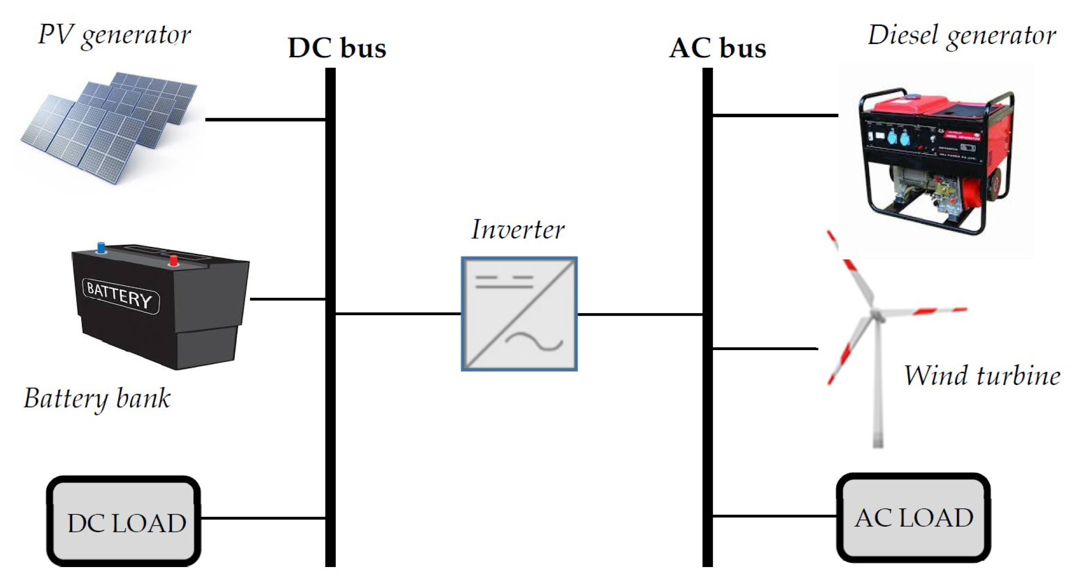
The microgrid considered for this study is located in the community of Nazareth (Department of La Guajira, Colombia), and its coordinates are latitude 12° 20′ 52.14″ N, longitude −71°16′8.80″ W. This place belongs to Colombia’s non-interconnected area (the Spanish acronym ZNI is used for these areas); however, it is located in a geographical place with a high potential for solar and wind resources, where proposals for microgrids have been made [33,34]. In addition, this area is characterized by not having 100% energy supply coverage. Figure 1 shows the microgrid.
The load profile is obtained according to the Energy Solutions data for the non-interconnected areas of Colombia IPSE (the government branch that plans and promotes these energy systems) [36], with an average temperature of 27 °C [37]. Table 1 shows the irradiation and wind data of the system installation site obtained from [38]. It can be seen that variation in irradiation and wind throughout the year is not very high. This situation is typical at latitudes close to the equator [39,40]. This small variability in wind and photovoltaic resources throughout the year allows for better use of renewable sources than at other latitudes [6]. The average daily electricity consumption is 30 kWh/day. The consumption is for households and street lighting. As it is an isolated microgrid, not interconnected with an electricity system, consumers of the microgrid cannot participate in the Colombian electricity market as self-consumers. The high number of areas not connected to the electricity grid is one of the most significant obstacles for renewable energy sources to participate in the Colombian electricity market [41].
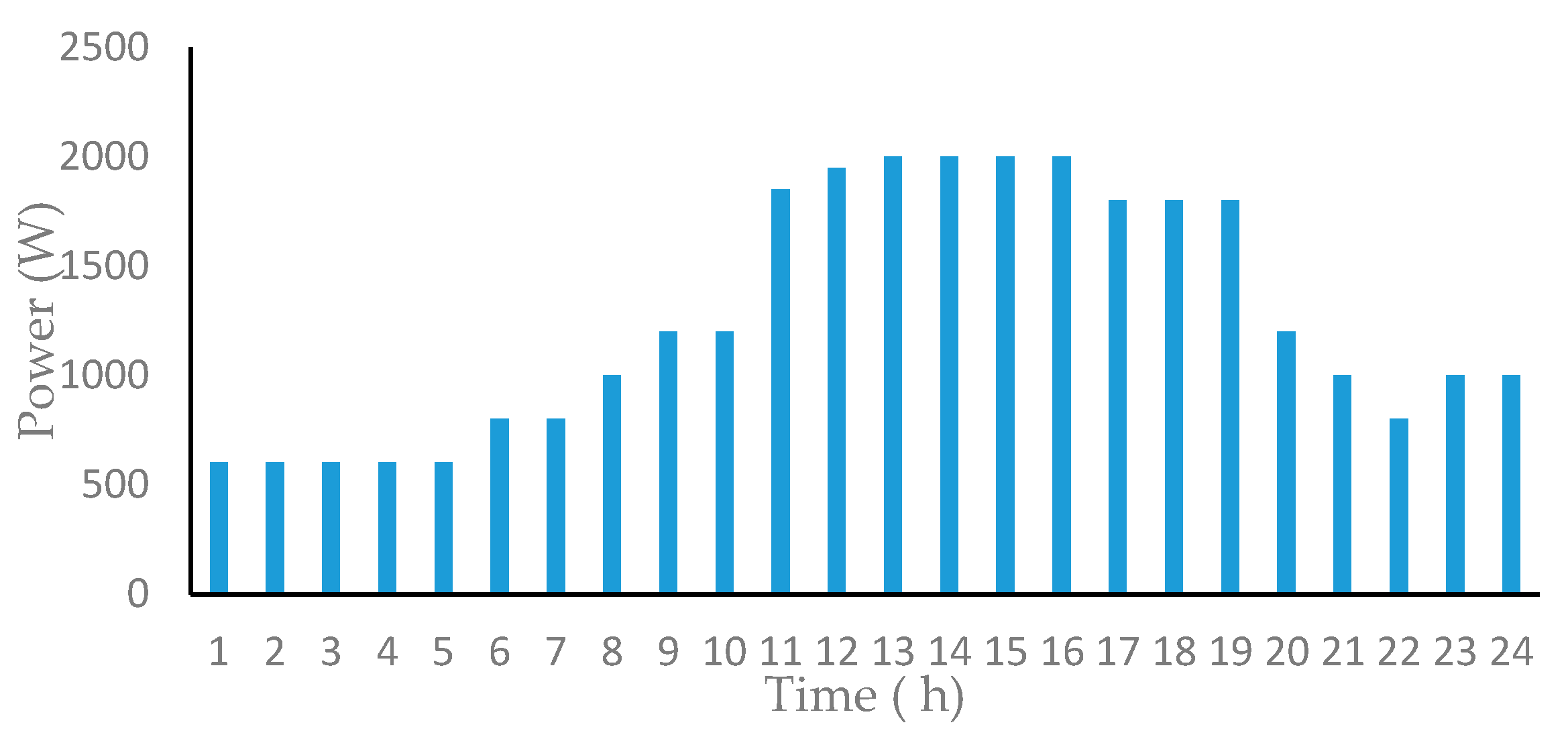
Figure 2 and Figure 3 show the wind speed and solar radiation values for 1 year at the simulated microgrid’s location. Figure 4 shows the load profile during a typical day.
The voltages in the microgrid are 48/220 V (CD/AC), the wind turbine power is 600 W, the inverter charger is 500 VA/48 V/70 A, the charge controller is PWM/48V/40A, and the diesel generator power is 1.6 kW. The other system data are summarized in Table 2 and Table 3.
The system’s lifetime is considered the same as a PV generator’s expected lifetime (the most common PV lifetime considered by researchers all around the world is 25 years). The economic data used to calculate the NPC of the actual system are shown in Table 4, obtaining the results of Section 3.1.
In this work, electricity supply optimization has been carried out for this case, considering various possibilities for the PV generator size, as well as for the wind turbine, diesel generator, and lead–acid batteries. In addition, various lithium battery sizes have been considered.
Table 5, Table 6, Table 7, Table 8 and Table 9 show, in detail, the parameters used in the optimization for each of the system components.
Optimization means also looking for the optimal control strategy between the two preselected options by the iHOGA software [42]. The two global strategies are as follow:
- Demand monitoring: Based on systems that include batteries and either diesel or gasoline generators, when the energy from renewable sources is not enough to meet the demand, the batteries will provide the rest of the energy. If the batteries cannot cover all of the demand, then the generator will work to meet the rest of the demand.
- Cyclic charging: If the generator is required to provide power, then it will only work at its nominal power not only to meet the demand but also to charge the batteries only during that hour. This strategy may have a variation called a cyclic strategy up to the setpoint, which means that the diesel generator will continue to operate at its nominal power until the battery bank reaches a specific value of SOC charge status, which is at 95% by default.
3. Results
3.1. Actual System
Table 10 shows the simulation results of the current system obtained from the data summarized in Section 2, considering different battery-aging models.
It is observed that the battery life is shorter with the Schiffer model (the most realistic model), and therefore more replacements are necessary throughout the system’s lifetime (25 years), so that NPC and LCOE are higher than using the other less realistic models.
3.2. System Optimization
Various optimizations have been made considering the different component options detailed in Section 2 (Table 5, Table 6, Table 7, Table 8 and Table 9). For each battery life model, two optimizations have been made, one for a hypothetical case of an average temperature of 20 °C and another for the real average temperature of the system’s location, which is 27 °C.
Table 11 shows the results for the microgrid optimization considering the three aging models for lead–acid batteries (equivalent cycle model, Rainflow, and Schiffer et al.). Classic models such as equivalent cycles and Rainflow present similar results, both in the expected lifetime as well as factors such as NPC and LCOE. These costs are higher when considering Schiffer’s aging model, which is more realistic, since decreasing the batteries’ lifetime would require more replacements during the project lifetime and therefore increase the total system cost.
It is also observed that using the equivalent cycle and Rainflow models, the battery lifetime is that of the floating lifetime since few cycles are performed per year. There is a reduction in the batteries’ lifetimes due to a 39.2% temperature increase using the real average temperature (27° at the installation site) compared to the case of 20 °C (the reduction is of the order of 50% for every 8.3 °C increase [43]). This reduction is much lower when using the Schiffer model since it considers many more parameters in addition to the temperature and cycles.
Considering the most realistic model (Schiffer) at the real average temperature (27 °C), the best system would be composed of the following: PV with 31.9 kWp capacity, diesel with 1.9 kVA capacity, wind with 660 W capacity, batteries with a 89.520 kWh energy storage capacity, inverter of 5 kVA capacity, with demand monitoring as the optimal control strategy, a battery life of 5.52 years, a NPC of €104,690, and an LCOE of €0.36/kWh. Compared to the result of the current system, considering the Schiffer model (Table 4), where the NPV is €119,458 and the LCOE is €0.49/kWh, it is observed that the current system is not optimal.
The results for one of the optimal cases obtained are shown in Figure 5 (with lead–acid batteries, Schiffer aging model, and at a temperature of 27 °C). The mono-objective optimization consists of obtaining the lowest NPC. The results show a minimum NPC of €104690 and an equivalent level of total CO2 emissions during the year of 1824 kg/year.
In Figure 5, the horizontal axis shows the generations of the evolutionary algorithm used by the iHOGA optimization software. An evolutionary algorithm generation is similar to an iteration [32].
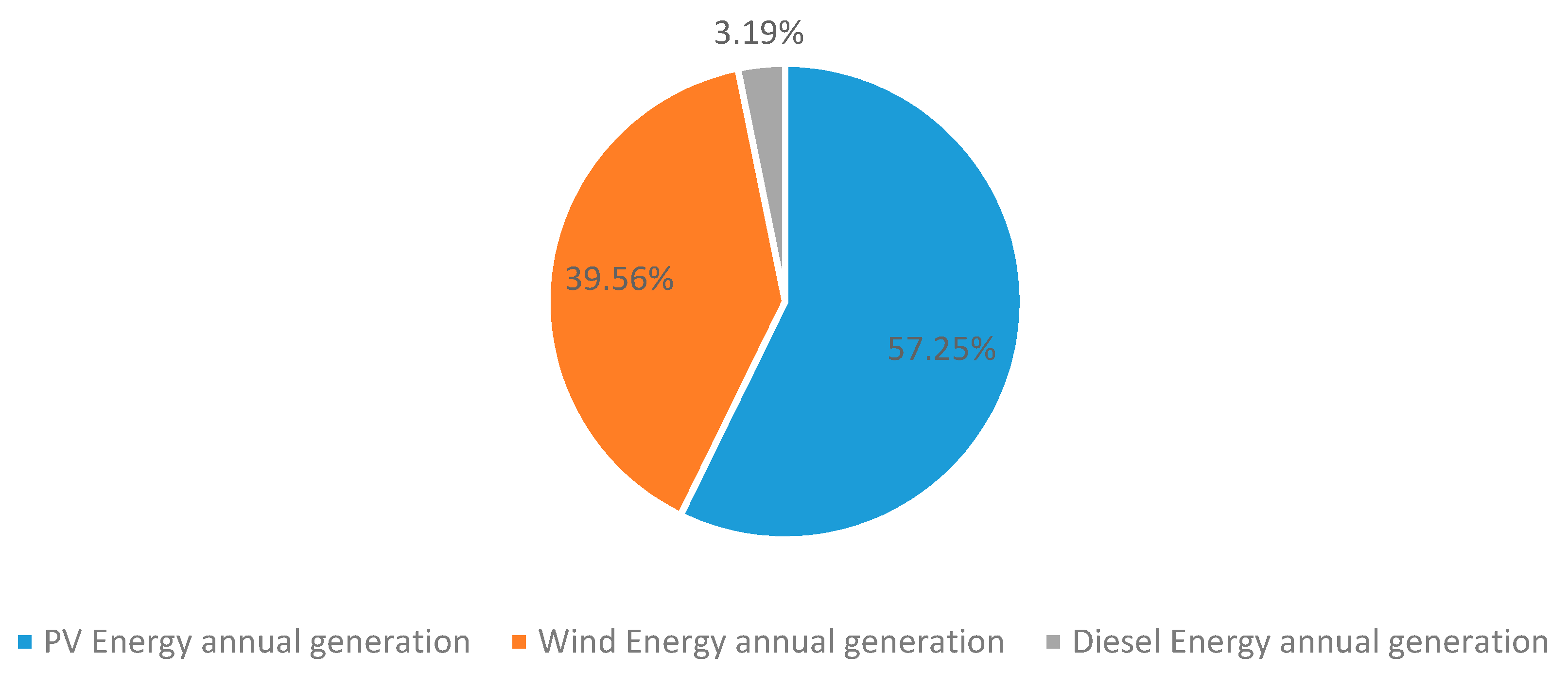
Figure 6 shows the annual distribution of energy generated in this case by the system for a year. The percentage of energy generated by renewables is 96.81%. Of this, 9703 kWh/year is supplied by the photovoltaic generator and 6705 kWh/year by wind turbines, while a smaller contribution is made by the 541 kWh/year diesel generator. The excess energy is 3496 kWh/year, which could be used to charge electric vehicles or to generate hydrogen, which could later be used in fuel-cell-powered electric vehicles [44].
The optimization results considering lithium batteries instead of lead–acid batteries are shown in Table 12. It is considered that the lithium batteries used can be LiFePO4/graphite or LiCoO2/graphite. Wang et al.’s model proved the most optimistic even when compared to the Groot model when the temperature rises, whereas Saxena’s model showed similar results for different temperatures because it is based on the SOC.
4. Discussion
In this work, different models and battery technologies have been compared in the optimization of a hybrid microgrid. The classic lead–acid battery aging models used by various researchers, such as the equivalent cycle model and the Rainflow cycle counting model, generally tend to overestimate the battery’s lifespan up to three times its actual duration. However, Schiffer et al.’s [13] weighted model has shown better results since their predictions are closer to the real ones. The results from the different optimizations show that lower net current costs (NPC) and lower LCOE are obtained for both lead–acid and lithium battery models; therefore, it is concluded that the current system is not optimized.
As for LiFePO4/graphite lithium–ferrophosphate batteries, Groot et al.’s [17] model presents more realistic results than Wang et al.’s [16] model, mainly due to temperature increases. Conversely, Saxena et al.’s [18] model showed the same results despite the variation in temperature, since the model is based on the SOC. Finally, comparing the two technologies (lead–acid vs. lithium), the results show lower NPC and LCOE costs for the case of lithium (compared to the realistic Schiffer model for lead–acid), which allows more optimistic insight into the exploration of new aging models for emerging technologies such as lithium batteries, as they represent an alternative storage technology for hybrid microgrids.
5. Conclusions
The most relevant conclusions of this work are as follows:
- Optimal dimensioning and management of the elements that make up a microgrid give rise to significant energy and economic benefits.
- Classic models for estimating battery life provide results that are too optimistic, so it is advisable to use models that are more realistic.
- The effect of temperature in the estimation of battery life can be significant, so models that consider this parameter should be used.
- Lithium-ion batteries are suitable as storage systems in a microgrid since they give rise to a lower cost throughout the life of the installation due to a longer lifespan than lead–acid batteries and a lower maintenance cost.
These conclusions allow us to state that it is necessary optimize the designs of microgrids not connected to the electricity grid since the economic benefits can be significant. An adequate design will allow for better use of renewable generation, and even take advantage of the surplus energy that can be used in electric vehicles, or in the case of islands, for water desalination. Furthermore, it is necessary to be open-minded and use other storage technologies, in addition to lead–acid batteries, since a lower initial cost does not imply that the total cost, throughout the life of the installation, will be low. Therefore, the use of other generation technologies, such as lithium-ion batteries, should be considered in the design, although their initial cost may be higher.
Author Contributions
Conceptualization, Y.E.G.-V. and R.D.-L.; methodology, Y.E.G.-V. and R.D.-L.; software, Y.E.G.-V. and R.D.-L.; validation, Y.E.G.-V., R.D.-L. and J.L.B.-A.; formal analysis, J.L.B.-A.; investigation, Y.E.G.-V.; resources, Y.E.G.-V.; data curation, Y.E.G.-V.; writing—original draft preparation, Y.E.G.-V.; writing—review and editing, R.D.-L. and J.L.B.-A.; visualization, R.D.-L. and J.L.B.-A.; supervision, R.D.-L. and J.L.B.-A. All authors have read and agreed to the published version of the manuscript.
Funding
This research received no external funding.
Conflicts of Interest
The authors declare no conflict of interest.
Nomenclature and Abbreviations
| a, b, C, d, e, f | adjustment constants |
| AFEC | Average Full Equivalent Cycles |
| Ah | amount of charge involved in the charging process since the start of battery operation (Ah) |
| Bcyc | exponential factor |
| CC | Cycle Charging |
| Ccorr | final loss of battery capacity due to continuous corrosion and degradation |
| Ccorr | loss of corrosion capacity |
| Cd (0) | initial normalized battery capacity |
| Cdeg | degradation capacity losses |
| CFi | cycles until failure for interval i |
| Costfuel | annual cost of the fuel used by the diesel generator (€) |
| CostINST | installation cost (€) |
| Costj | acquisition cost of component j (€) |
| CostO&Mj | annual O&M cost of component j (€) |
| Cn | nominal capacity of a battery (Ah) |
| DOD | Depth of Discharge (%) |
| Eacyc | activation energy expressed in J mol−1 |
| EFC | Equivalent Full Cycles |
| Eload | annual expected load of the system (kWh/yr) |
| iHOGA | improved Hybrid optimization by genetic algorithms |
| HOMER | Hybrid optimization model for multiple energy resources |
| I | charge rate (A) |
| IEC | International Electrotechnical Commission |
| Inffuel | annual expected diesel fuel inflation (€) |
| Infgeneral | general annual expected inflation (%) |
| IPSE | Instituto de Planificación y Promoción de Soluciones Energéticas para las Zonas No Interconectadas |
| Ir | annual interest rate (%) |
| Isc | PV module short current (A) |
| LCOE | Levelized Cost of Energy |
| LCOEi,k | LCOE (€/kWh) of a combination of components i and control strategy k |
| LF | Load Following |
| Lifebat | battery life (h) |
| NOCT | Nominal operation cell temperature (°C) |
| NPC | Net Present Cost (€) |
| NPCi,k | NPC (€) of a combination of components i and control strategy k |
| NPCrepj | sum of the replacement costs of component j during the system lifetime minus the residual cost of component j at the end of the system lifetime (€) |
| O&M | operating and maintenance costs |
| PV | Photovoltaic |
| QEOL | charge that the battery can deliver in its lifetime (kAh) |
| Qloss | percentage of capacity loss (%) |
| percentage of capacity loss (%) | |
| R | gas constant (8.314 J·mol−1·K−1) |
| RCC | Rainflow Cycle Counting |
| Schiffer# | Schiffer without continuing up to SOC setpoint |
| SOC | State of Charge (%) |
| SOCmean | average SOC (30%–50%) |
| SOCmin | minimum SOC allowed |
| SOCst | SOC at which the battery is stored (%) |
| t | elapsed time, in hours |
| T | temperature (K, °C) |
| tm | storage time, in months |
| ty | one year of the system lifetime |
| Voc | PV module open-circuit voltage (V) |
| Zcyc | constant with a value close to 0.5 |
| Zi | cycle count |
| ZIEC | number of cycles provided by the manufacturer to reach the end of the battery life. |
| number of complete cycles | |
| γ | coefficient to determine the acceleration in aging due to the current (J mol−1 A−1) |
| α | PV module temperature coefficient (%/°C) |
| ΔSOC | variation of the SOC (100%–60%) |
| absolute value of the discharge current (A) |
References
- International Energy Agency (IEA). World Energy Outlook. Available online: https://www.iea.org/reports/world-energy-outlook-2019/renewables (accessed on 3 November 2019).
- U.S. Energy; Administration, I. DOE-EIA International Energy Outlook. 2019. Available online: www.eia.gov/ieo (accessed on 10 December 2019).
- Zsiborács, H.; Baranyai, N.H.; Vincze, A.; Zentkó, L.; Birkner, Z.; Máté, K.; Pintér, G. Intermittent renewable energy sources: The role of energy storage in the european power system of 2040. Electron 2019, 8. [Google Scholar] [CrossRef] [Green Version]
- Bakić, V.; Pezo, M.; Stevanović, Ž.; Živković, M.; Grubor, B. Dynamical simulation of PV/Wind hybrid energy conversion system. Energy 2012, 45, 324–328. [Google Scholar] [CrossRef]
- Huang, Q.; Shi, Y.; Wang, Y.; Lu, L.; Cui, Y. Multi-turbine wind-solar hybrid system. Renew. Energy 2015, 76, 401–407. [Google Scholar] [CrossRef]
- Uche, J.; Acevedo, L.; Círez, F.; Usón, S.; Martínez-Gracia, A.; Bayod-Rújula, Á.A. Analysis of a domestic trigeneration scheme with hybrid renewable energy sources and desalting techniques. J. Clean. Prod. 2019, 212, 1409–1422. [Google Scholar] [CrossRef] [Green Version]
- Fadaeenejad, M.; Radzi, M.A.M.; Abkadir, M.Z.A.; Hizam, H. Assessment of hybrid renewable power sources for rural electrification in Malaysia. Renew. Sustain. Energy Rev. 2014, 30, 299–305. [Google Scholar] [CrossRef]
- García Vera, Y.E.; Dufo-López, R.; Bernal-Agustín, J.L. Energy management in microgrids with renewable energy sources: A literature review. Appl. Sci. 2019, 9. [Google Scholar] [CrossRef] [Green Version]
- Jaiswal, A. Lithium-ion battery based renewable energy solution for off-grid electricity: A techno-economic analysis. Renew. Sustain. Energy Rev. 2017, 72, 922–934. [Google Scholar] [CrossRef]
- Lai, C.S.; Jia, Y.; Xu, Z.; Lai, L.L.; Li, X.; Cao, J.; McCulloch, M.D. Levelized cost of electricity for photovoltaic/biogas power plant hybrid system with electrical energy storage degradation costs. Energy Convers. Manag. 2017, 153, 34–47. [Google Scholar] [CrossRef]
- Drouilhet, S.; Johnson, B.L. A battery life prediction method for hybrid power applications. In Proceedings of the 35th Aerospace Sciences Meeting and Exhibit, Reno, NV, USA, 6–9 January 1997. [Google Scholar]
- Jenkins, D.P.; Fletcher, J.; Kane, D. Lifetime prediction and sizing of lead-acid batteries for microgeneration storage applications. IET Renew. Power Gener. 2008, 2, 191–200. [Google Scholar] [CrossRef]
- Schiffer, J.; Sauer, D.U.; Bindner, H.; Cronin, T.; Lundsager, P.; Kaiser, R. Model prediction for ranking lead-acid batteries according to expected lifetime in renewable energy systems and autonomous power-supply systems. J. Power Sources 2007, 168, 66–78. [Google Scholar] [CrossRef]
- Dufo-López, R.; Lujano-Rojas, J.M.; Bernal-Agustín, J.L. Comparison of different lead-acid battery lifetime prediction models for use in simulation of stand-alone photovoltaic systems. Appl. Energy 2014, 115, 242–253. [Google Scholar] [CrossRef]
- Dufo-López, R. iHOGA. Available online: https://ihoga.unizar.es/en/ (accessed on 3 April 2019).
- Wang, J.; Liu, P.; Hicks-Garner, J.; Sherman, E.; Soukiazian, S.; Verbrugge, M.; Tataria, H.; Musser, J.; Finamore, P. Cycle-life model for graphite-LiFePO4 cells. J. Power Sources 2011, 196, 3942–3948. [Google Scholar] [CrossRef]
- Groot, J.; Swierczynski, M.; Stan, A.I.; Kær, S.K. On the complex ageing characteristics of high-power LiFePO4/graphite battery cells cycled with high charge and discharge currents. J. Power Sources 2015, 286, 475–487. [Google Scholar] [CrossRef]
- Saxena, S.; Hendricks, C.; Pecht, M. Cycle life testing and modeling of graphite/LiCoO2 cells under different state of charge ranges. J. Power Sources 2016, 327, 394–400. [Google Scholar] [CrossRef]
- Cristóbal-Monreal, I.R.; Dufo-López, R.; Yusta-Loyo, J.M. Influence of the battery model in the optimisation of stand-alone renewable systems. Renew. Energy Power Qual. J. 2016. [Google Scholar] [CrossRef]
- Zhao, B.; Zhang, X.; Chen, J.; Wang, C.; Guo, L. Operation optimization of standalone microgrids considering lifetime characteristics of battery energy storage system. IEEE Trans. Sustain. Energy 2013, 4, 934–943. [Google Scholar] [CrossRef]
- Keshan, H.; Thornburg, J.; Ustun, T.S. Comparison of Lead-Acid and Lithium Ion Batteries for Stationary Storage in Off-Grid Energy Systems. In Proceedings of the 4th IET Clean Energy and Technology Conference (CEAT 2016), Kuala Lumpur, Malaysia, 14–15 November 2016; p. 7. [Google Scholar]
- Anuphappharadorn, S.; Sukchai, S.; Sirisamphanwong, C.; Ketjoy, N. Comparison the economic analysis of the battery between lithium-ion and lead-acid in PV stand-alone application. Energy Procedia 2014, 56, 352–358. [Google Scholar] [CrossRef] [Green Version]
- Dufo-López, R.; Cristóbal-Monreal, I.R.; Yusta, J.M. Optimisation of PV-wind-diesel-battery stand-alone systems to minimise cost and maximise human development index and job creation. Renew. Energy 2016, 94, 280–293. [Google Scholar] [CrossRef]
- Lujano-Rojas, J.M.; Dufo-López, R.; Bernal-Agustín, J.L. Optimal sizing of small wind/battery systems considering the DC bus voltage stability effect on energy capture, wind speed variability, and load uncertainty. Appl. Energy 2012, 93, 404–412. [Google Scholar] [CrossRef]
- Ruetschi, P. Aging mechanisms and service life of lead-acid batteries. J. Power Sources 2004, 127, 33–44. [Google Scholar] [CrossRef]
- Astaneh, M.; Dufo-López, R.; Roshandel, R.; Bernal-Agustin, J.L. A novel lifetime prediction method for lithium-ion batteries in the case of stand-alone renewable energy systems. Int. J. Electr. Power Energy Syst. 2018, 103, 115–126. [Google Scholar] [CrossRef]
- HOMER Energy. HOMER (Hybrid Optimization of Multiple Energy Resources). Available online: https://www.homerenergy.com (accessed on 6 June 2019).
- IEC 60896-11 Stationary Lead-Acid Batteries–Part 11: Vented Types–General Requirements and Methods of Tests; IEC: Geneva, Switzerland, 2002; Volume 39.
- Downing, S.D.; Socie, D.F. Simple rainflow counting algorithms. Int. J. Fatigue 1982, 4, 31–40. [Google Scholar] [CrossRef]
- Petit, M.; Prada, E.; Sauvant-Moynot, V. Development of an empirical aging model for Li-ion batteries and application to assess the impact of Vehicle-to-Grid strategies on battery lifetime. Appl. Energy 2016, 172, 398–407. [Google Scholar] [CrossRef]
- Swierczynski, M.; Stroe, D.I.; Stan, A.I.; Teodorescu, R.; Kær, S.K. Lifetime Estimation of the Nanophosphate LiFePO4/C Battery Chemistry Used in Fully Electric Vehicles. IEEE Trans. Ind. Appl. 2015, 51, 3453–3461. [Google Scholar] [CrossRef]
- Goldberg, D.E. Genetic Algorithms in Search, Optimization, and Machine Leaming; Addison Wesley Publishing Company, Inc.: Boston, MA, USA, 1989; ISBN 0201157675. [Google Scholar]
- Garzón-Hidalgo, J.D.; Andrés, Y.; Saavedra-Montes, J. A design methodology of microgrids for non- interconnected zones of Colombia. Tecnológicas 2017, 20. [Google Scholar] [CrossRef] [Green Version]
- Tello-Maita, J.; Marulanda-Guerra, A. Optimization models for power systems in the evolution to smart grids: A review. DYNA 2017, 84, 102–111. [Google Scholar]
- IPSE (Instituto de Planificación y Promoción de Soluciones Energéticas para las Zonas No Interconectadas). Soluciones energéticas para las zonas no interconectadas de Colombia IPSE. Available online: https://docplayer.es/storage/38/17971329/1578394308/gRMnLy8ukBAZTkZv7tN5NA/17971329.pdf (accessed on 3 June 2019).
- IPSE (Instituto de Planificación y Promoción de Soluciones Energéticas para las Zonas No Interconectadas). Centro Nacional de Monitoreo. Available online: http://190.216.196.84/cnm/cnm.php (accessed on 7 November 2019).
- IDEAM (Instituto de Hidrología, Meteorología y Estudios Ambientales). Indicadores y estadísticas ambientales. Available online: http://www.ideam.gov.co/ (accessed on 7 November 2019).
- NASA. Nasa Predicition of Worldwide Energy Resources. Available online: https://power.larc.nasa.gov/ (accessed on 3 July 2019).
- López-García, D.; Arango-Manrique, A.; Carvajal-Quintero, S.X. Integration of distributed energy resources in isolated microgrids: The Colombian paradigm. TecnoLógicas 2018, 21, 13–30. [Google Scholar]
- Aristizábal, A.J.; Herrera, J.; Castaneda, M.; Zapata, S.; Ospina, D.; Banguero, E. A new methodology to model and simulate microgrids operating in low latitude countries. Energy Procedia 2019, 157, 825–836. [Google Scholar] [CrossRef]
- Gómez-Navarro, T.; Ribó-Pérez, D. Assessing the obstacles to the participation of renewable energy sources in the electricity market of Colombia. Renew. Sustain. Energy Rev. 2018, 90, 131–141. [Google Scholar] [CrossRef]
- Dufo-López, R.; Bernal-Agustín, J.L. Design and control strategies of PV-Diesel systems using genetic algorithms. Sol. Energy 2005, 79, 33–46. [Google Scholar] [CrossRef]
- 1187–2013–IEEE Recommended Practice for Installation Design and Installation of Valve-Regulated Lead-Acid Batteries for Stationary Applications; IEEE SA: Piscataway, NJ, USA, 2014.
- Carroquino, J.; Bernal-Agustín, J.L.; Dufo-López, R. Standalone Renewable Energy and Hydrogen in an Agricultural Context: A Demonstrative Case. Sustainability 2019, 11, 951. [Google Scholar] [CrossRef] [Green Version]
Figure 1.
Nazareth microgrid [35].
Figure 1.
Nazareth microgrid [35].

Figure 2.
Wind speed (in an average year) at the microgrid location.

Figure 3.
Hourly solar irradiation (in an average year) and detail for a specific day at the grid location.
Figure 3.
Hourly solar irradiation (in an average year) and detail for a specific day at the grid location.
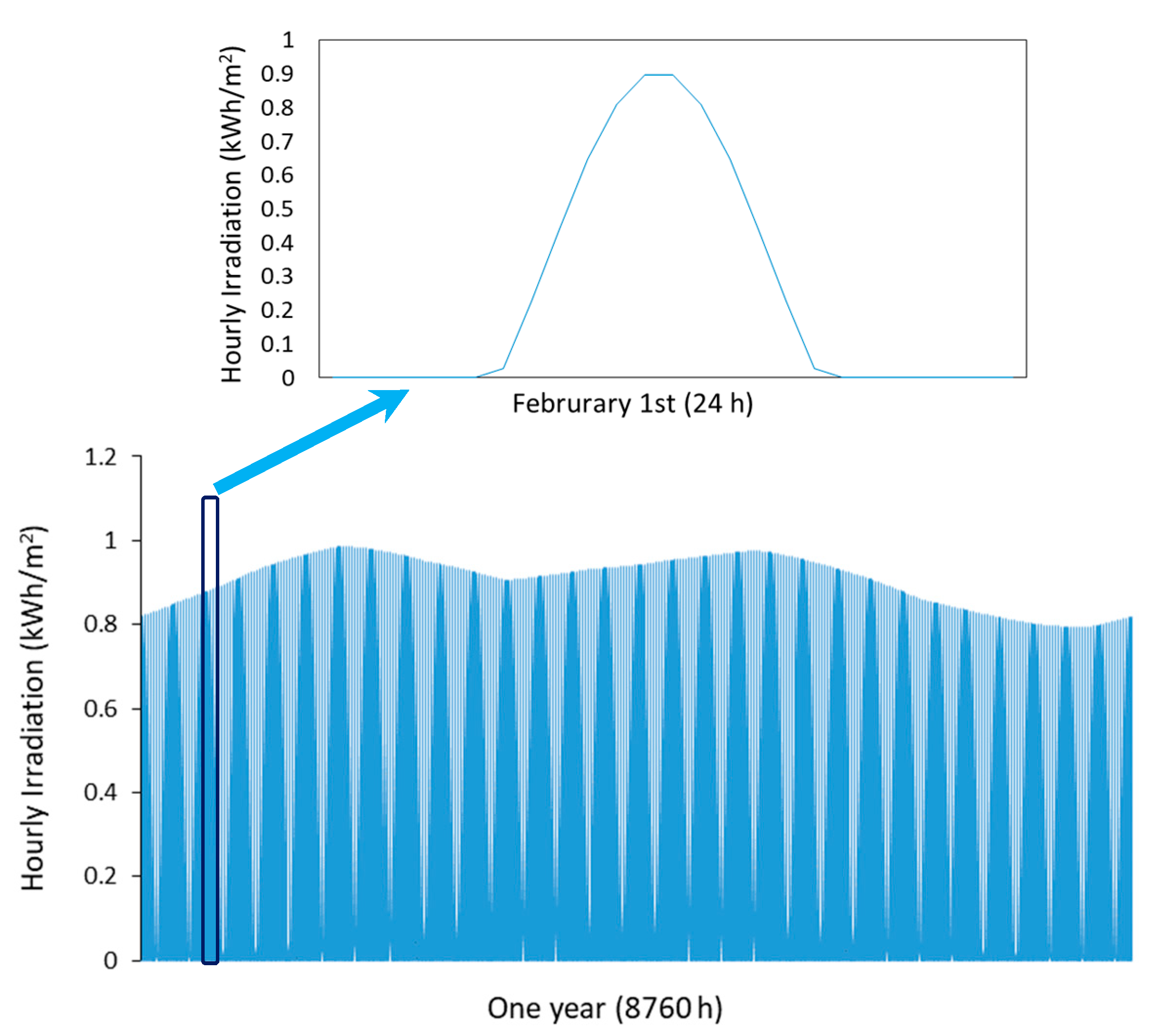
Figure 4.
Typical daily load profile for the case study at the grid location.

Figure 5.
Results for NPC and CO2 emissions for every generation.
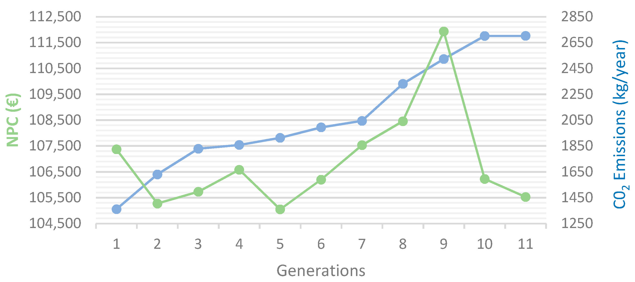
Figure 6.
Annual energy distribution.

Table 1.
Irradiation and wind speed at the microgrid location.
| Month | Irradiation (kWh/m2/day) | Wind Speed (m/s) |
|---|---|---|
| January | 5.86 | 7.04 |
| February | 6.51 | 7.24 |
| March | 7.02 | 7.1 |
| April | 6.92 | 6.93 |
| May | 6.72 | 6.86 |
| June | 7 | 7.64 |
| July | 7.13 | 7.39 |
| August | 7.17 | 6.62 |
| September | 6.66 | 5.7 |
| October | 5.99 | 5.25 |
| November | 5.57 | 5.75 |
| December | 5.39 | 6.7 |
Table 2.
Photovoltaic (PV) data of the simulated microgrid.
| PV Module Type | Monocrystalline |
|---|---|
| PV module power (Wp) | 380 |
| Number of PV modules in serial/Parallel | 2/22 |
| PV module short current Isc (A) | 10.11 |
| PV module open-circuit voltage Voc(V) | 24 |
| PV module temperature coefficient (%/°C) | −0.37 |
| NOCT (°C) | 48° |
| PV module slope | 15° |
| PV module azimuth | 0° |
Table 3.
Batteries data.
| Battery Type | OPZS |
|---|---|
| Number of batteries in serial/parallel | 24/1 |
| Battery voltage (V) | 2 |
| Battery capacity C10 (Ah) | 3360 |
| Battery float life at 20 °C (years) | 15 |
| Battery equivalent full cycles | 1500 |
Table 4.
Economic data for net present cost (NPC) calculation.
| Parameters | Economic Data |
|---|---|
| Battery bank acquisition cost | 30,960 € |
| PV generator acquisition cost | 9680 € |
| PV generator expected lifetime | 25 years |
| Diesel generator acquisition | 800 € |
| Diesel generator expected lifetime | 10,000 h |
| Inverter acquisition cost | 2915 € |
| Wind turbine acquisition cost | 4255 € |
| Wind turbine generator expected lifetime | 15 years |
| Controller acquisition cost | 2215 € |
| Expected controlled and inverter lifetime | 10 year |
| The lifetime of the system | 25 years |
| Average annual interest rate/inflation rate | 4%/4% |
| Installation cost | 500 € |
Table 5.
PV modules considered in the optimization.
| Parameters | Data |
|---|---|
| Nominal Power | 380 Wp |
| Isc | 10.11 A |
| NOCT | 47° |
| α | −0.37%/°C |
| Acquisition cost | 220 € |
| Lifespan | 25 years |
| Nominal voltage (2 in serial) | 24 V |
| Maximum number allowed | 2 in serial/50 in parallel |
Table 6.
Wind turbines used in optimization.
| Parameters | Model 1: WT600 | Model 2: WT3000 |
|---|---|---|
| Maximum power | 660 W | 3471 W |
| Hub height | 13 m | 15 m |
| Acquisition cost | 4255 € | 7555 € |
| Lifespan | 15 years | 15 years |
| O&M cost | 85 €/year | 50 €/year |
| Maximum number allowed in parallel | 3 | 3 |
Table 7.
Batteries used in the optimization.
| Parameters | Lead–Acid 1 | Lead–Acid 2 | Lithium 1 | Lithium 2 |
|---|---|---|---|---|
| OPZS | OPZS | BYD B-Box 5.0 | LG Chem | |
| Capacity | 1865 Ah | 3360 Ah | 106.6 Ah | 63 Ah |
| Acquisition cost | 820 € | 1010 € | 3390 € | 3400 € |
| O&M cost (one cell) | 8.2 €/year | 10.1 €/year | 20 €/year | 30 €/year |
| O&M cost (whole bank) * | 50 €/year | 50 €/year | 50 €/year | 50 €/year |
| Nominal voltage | 2 V | 2 V | 48 V | 48 V |
| Float life at 20 °C | 20 years | 18 years | 10 years | 10 years |
| Equivalent full cycles | 1500 | 1600 | 6000 | 3200 |
| SOCmin | 20% | 20% | 20% | 20% |
| Self-discharge | 3%/month | 3%/month | 2%/month | 2%/month |
| Number of series batteries | 24 | 24 | 1 | 1 |
| Maximum number in parallel | 6 | 6 | 6 | 6 |
* Cost of the maintenance technician’s journey.
Table 8.
Diesel generator considered in the optimization.
| Parameters | Data |
|---|---|
| Nominal Power | 1.9 kVA |
| Minimal power | 30% |
| Acquisition cost | 800 € |
| Lifespan | 10,000 h |
| O&M cost | 0.14 €/h |
| Diesel fuel cost (including transportation) | 1.13 €/l |
| Maximum number allowed in parallel | 2 |
Table 9.
Inverter/charger considered in the optimization.
| Nominal Power | 5 kVA |
| Efficiency | 90% |
Table 10.
Simulation results for the current system, using the three lead–acid battery-aging models and an average ambient temperature of 27°.
Table 10.
Simulation results for the current system, using the three lead–acid battery-aging models and an average ambient temperature of 27°.
| Battery-Aging Model | Lifespan | NPC | LCOE |
|---|---|---|---|
| (years) | (€) | (€/kWh) | |
| Rainflow cycle counting | 9.23 | 98,891 | 0.36 |
| Average full equivalent cycles | 9.23 | 99,061 | 0.36 |
| Schiffer | 7.05 | 119,458 | 0.49 |
Table 11.
Results of the system optimizations in the case of lead–acid batteries, using the three battery life models and with two different values of average ambient temperature (20 °C or 27 °C).
Table 11.
Results of the system optimizations in the case of lead–acid batteries, using the three battery life models and with two different values of average ambient temperature (20 °C or 27 °C).
| Battery Aging Model 1 | Ambient Temp. | Optimal System Configuration 2 (In all cases: Diesel Generator Power = 1.9 kVA, Battery Bank Capacity = 89.52 kWh, and Inverter Power = 5 kVA) | Control Strategy 3 | Lifetime (Years) | NPC (€) | LCOE (€/kWh) |
|---|---|---|---|---|---|---|
| AFEC | 20° | 12.16 kWp/0 kW | LF | 20 | 52,544 | 0.19 |
| AFEC | 27° | 12.16 kWp/0 kW | LF | 12.31 | 59,413 | 0.21 |
| RCC | 20° | 34.2 kWp/0 kW | LF | 20 | 52,013 | 0.19 |
| RCC | 27° | 33.4 kWp/0 kW | LF | 12.31 | 59,413 | 0.21 |
| Schiffer | 20° | 32.68 kWp/0 kW | LF | 7.73 | 91,573 | 0.32 |
| Schiffer | 20° | 32.68 kWp/0 kW | CC | 7.59 | 92,195 | 0.32 |
| Schiffer# | 20° | 32.44 kWp/0 kW | CC | 7.36 | 92,650 | 0.32 |
| Schiffer | 27° | 31.9 kWp/660 kW | LF | 5.52 | 104,690 | 0.36 |
| Schiffer | 27º | 29.64 kWp/660 kW | CC | 5.67 | 104,730 | 0.36 |
| Schiffer# | 27º | 29.64 kWp/660 kW | CC | 5.63 | 105,307 | 0.36 |
1 AFEC = average full equivalent cycles. RCC = rainflow cycle counting. Schiffer# = Schiffer without continuing up to SOC setpoint.; 2 PV power (kWp)/Wind turbine power (kW).; 3 LF = load following. CC = cycle charging.
Table 12.
Results of the optimizations for the case of lithium batteries, using the three models of battery life and with two different average ambient temperature values (20 °C or 27 °C).
Table 12.
Results of the optimizations for the case of lithium batteries, using the three models of battery life and with two different average ambient temperature values (20 °C or 27 °C).
| Battery Aging Model 1 | Ambient Temp. | Optimal System Configuration 2 (In all Cases, Inverter Power = 5 kVA) | Control Strategy 3 | Lifetime (Years) | NPC (€) | LCOE (€/kWh) |
|---|---|---|---|---|---|---|
| Wang | 20° | 14.44 kWp/1.9 kVA/0 kW/15.35 kWh | LF | 10 | 47,889 | 0.17 |
| Wang | 20° | 15.2 kWp/1.9 kVA/0 kW/20.46 kWh | CC | 10 | 52,657 | 0.18 |
| Wang | 27° | 14.44 kWp/1.9 kVA/1.66 kW/15.35 kWh | LF | 6.15 | 56,204 | 0.20 |
| Wang | 27° | 13.68 kWp/1.9 kVA/1.66 kW/15.35 kWh | CC | 6.12 | 64,796 | 0.23 |
| Groot | 20° | 14.44 kWp/1.9 kVA/0 kW/15.35 kWh | LF | 10 | 47,934 | 0.17 |
| Groot | 20° | PV 15.2 kWp/1.9 kVA/0 kW/20.4 kWh | CC | 10 | 52,657 | 0.19 |
| Groot | 27° | 14.44 kWp/1.9 kVA/0 kW/15.35 kWh | LF | 6.15 | 56,204 | 0.20 |
| Groot | 27° | 15.2 kWp/1.9 kVA/0 kW/20.4 kWh | CC | 6.15 | 63,747 | 0.23 |
| Saxena | 20° | 13.68 kWp/1.9 kVA/0 kW/15.35 kWh | LF | 3 | 78,427 | 0.29 |
| Saxena | 27° | 19 kWp/1.9 kVA/3.32 kW/15.35 kWh | LF | 3.03 | 84,742 | 0.22 |
| AFEC | 20° | 20.52 kWp/1.9 kVA/1.66 kW/10.2 kWh | LF | 10 | 54,216 | 0.19 |
| AFEC | 27° | 13.68 kWp/3.8 kVA/3.32 kW/5.1 kWh | LF | 6.15. | 58,216 | 0.2 |
| AFEC | 27° | 15.2 kWp/1.9 kVA/0 kW/20.4 kWh | CC | 6.15. | 63,747 | 0.23 |
| RCC | 20º | 14.44 kWp/1.9 kVA/0 kW/15.3 kWh | LF | 9.88 | 48,455 | 0.18 |
| RCC | 20º | 15.2 kWp/1.9 kVA/0 kW/20.4 kWh | CC | 9.88 | 53,461 | 0.19 |
| RCC | 27º | 14.44 kWp/3.8 kVA/3.32 kW/5.1 kWh | LF | 6.15 | 57,162 | 0.2 |
1 AFEC = average full equivalent cycles. RCC = rainflow cycle counting.; 2 PV power (kWp)/Diesel generator power (kVA)/Wind turbine power (kW)/Battery bank capacity (kWh); 3 LF = load following. CC = cycle charging.
© 2020 by the authors. Licensee MDPI, Basel, Switzerland. This article is an open access article distributed under the terms and conditions of the Creative Commons Attribution (CC BY) license (http://creativecommons.org/licenses/by/4.0/).
Share and Cite
MDPI and ACS Style
García-Vera, Y.E.; Dufo-López, R.; Bernal-Agustín, J.L. Optimization of Isolated Hybrid Microgrids with Renewable Energy Based on Different Battery Models and Technologies. Energies 2020, 13, 581. https://doi.org/10.3390/en13030581
AMA Style
García-Vera YE, Dufo-López R, Bernal-Agustín JL. Optimization of Isolated Hybrid Microgrids with Renewable Energy Based on Different Battery Models and Technologies. Energies. 2020; 13(3):581. https://doi.org/10.3390/en13030581
Chicago/Turabian StyleGarcía-Vera, Yimy E., Rodolfo Dufo-López, and José L. Bernal-Agustín. 2020. "Optimization of Isolated Hybrid Microgrids with Renewable Energy Based on Different Battery Models and Technologies" Energies 13, no. 3: 581. https://doi.org/10.3390/en13030581
Note that from the first issue of 2016, this journal uses article numbers instead of page numbers. See further details here.