Article

Heuristic Optimization of Virtual Inertia Control in Grid-Connected Wind Energy Conversion Systems for Frequency Support in a Restructured Environment

by
Anuoluwapo Oluwatobiloba Aluko
1,*,
David George Dorrell
1,
Rudiren Pillay Carpanen
1 and
Evan E. Ojo
2
1
Discipline of Electrical, Electronic and Computer Engineering, University of KwaZulu-Natal, Durban 4041, KwaZulu-Natal, South Africa
2
Department of Electrical Power Engineering, Durban University of Technology, Durban 4000, KwaZulu-Natal, South Africa
*
Author to whom correspondence should be addressed.
Energies 2020, 13(3), 564; https://doi.org/10.3390/en13030564
Submission received: 19 November 2019 / Revised: 1 January 2020 / Accepted: 8 January 2020 / Published: 24 January 2020
(This article belongs to the Special Issue Heuristic Optimization Techniques Applied to Power Systems)

Abstract

:
In the work reported in this paper, a novel application of the artificial bee colony algorithm is used to implement a virtual inertia control strategy for grid-connected wind energy conversion systems. The proposed control strategy introduces a new heuristic optimization technique that uses the artificial bee colony (ABC) algorithm to calculate the optimal gain value of an additional derivative control loop added to the control scheme of the machine side converter in a wind energy system to enable wind farms to participate in frequency control as specified by recent grid codes. This helps to minimize the frequency deviations, reduce active power deviation in the system, and increase the penetration level of wind energy in power systems. The study was performed in a restructured power system environment. The proposed control scheme and its robustness were evaluated using load–frequency analysis for three real-life transaction scenarios that can occur in an interconnected open-energy market and the validation was carried out using eigenvalue analysis. The results in this study show that the optimal gain of the proposed controller reduces the frequency deviations and improves stability and overall performance of the system.

Graphical Abstract

1. Introduction

To meet increasing load demand and reduce environmental pollution caused by fossil-fuelled power plants, power generation from renewable sources has become a viable solution in many instances. Modern power systems consist of many control areas with different sources of generation [1]. Any variance between the generated power and required load demand results in the deviation of the system frequency from its nominal value. This also creates an inadvertent exchange of power between interconnected control areas. The intrinsic characteristic of conventional generators that make them applicable for frequency control is “inertia”. The large moment of inertia present in synchronous generators allows conventional/traditional power systems to maintain stability during disturbance as a result of frequency regulation action. In the past, the impacts of renewable energy plants (REPs) in large power systems were considered negligible because of low-level penetration. With the increasing penetration of REPs, most countries have developed renewable energy grid codes that REPs seeking connection to the grid must comply with [2,3,4]. In a similar manner to codes for conventional plants, REPs grid codes specify that some ancillary services must be provided during transient conditions [5]. One of these ancillary services is frequency control. Depending on the amplitude and duration of the frequency deviation, frequency control can be classified into primary, secondary, tertiary, and emergency frequency control [6]. This study is concerned with the impacts of inertia on primary and secondary frequency control because the efficiency of these controls can mitigate against the need for a higher level of frequency control. Primary frequency control is able to attenuate small frequency deviation but is not able to restore the system to the nominal frequency; thus, secondary frequency control is activated by harnessing the available power reserve to restore the system to nominal operating frequency. Secondary frequency control is also known as automatic generation control (AGC) or load frequency control (LFC). This is now becoming a complex control problem in power system design, operation, and control because of the emerging complexities such as renewable energy penetration, deregulation, new standards, environmental constraints, and various uncertainties [7]. Early studies on LFC problems focused on a single-area power systems with conventional power plant generation [8,9,10]; LFC models for hydropower plants were introduced in [11,12,13]. By interconnecting power systems, reliability and resilience are improved because there is inter-area support during deviating conditions. High voltage AC (HVAC) tie lines are used for interconnection in traditional power systems; the effects of HVAC tie line models were investigated in [14,15]. Studies for a two-area power system considering conventional multi-source plants were presented in [16,17,18,19,20] and higher-order interconnected areas were studied in [21,22,23,24,25,26]. The application of HVAC lines for long-distance transmission is associated with several drawbacks such as effect of capacitance for underground transmission [27], line inductance [28], Ferranti effect [29], asynchronous interconnection [30], and reduce active power transmission-to-length ratio [31]. Modern power systems have adopted the application of high voltage DC (HVDC) transmission link for long distance transmission to provide solutions to inherent HVAC transmission problems. This leads to economic and technical advantages [30,32,33].
In the traditional power system environment, the vertically integrated utility (VIU) solely owns the generation companies (GENCOs), transmission companies (TRANSCOs), and distribution companies (DISCOs), which supply power to clients at regulated prices [34,35]. The physical boundaries of a VIU define the control areas which are interconnected via tie lines. In a restructured or deregulated environment, GENCOs may choose to participate in frequency regulation, and independent power producers (IPPs) or REPs seeking connection to the grid must meet the grid code requirements by providing frequency support to the system during disturbances. DISCOs have the freedom to individually contract power from GENCOs and IPPs in different areas. The transactions among the GENCOs, IPPs, and DISCOs are supervised by an independent system operator (ISO) or any other transparent organization [6]. Provision of ancillary services such as frequency control is optional and usually based on competitive pricing, thus it is regarded as an open energy market [36]. Frequency response models for power systems in a deregulated environment must consider the contracts between DISCOs and GENCOs; Sekhar et al. [37] investigated LFC models for hydro plants. Thermal plants were considered in [38] and multi-sources were studied in [39].
In modern power systems, the impacts of REPs can no longer be considered negligible because of the increased level of penetration. The increasing integration of renewable energy plants (almost zero-inertia) reduces the overall inertia of the system, which makes the system more susceptible to high transient frequency deviations, thus making LFC problems more complex [40]. The reduction in inertia causes some problems in the deregulated environment for the ISO, such as a reduction in frequency and system oscillation. Due to the rotational parts present in wind energy conversion systems, recent grid codes require that they participate in frequency regulation within a specified range [41]. Anaya-Lara et al. [42] investigated the capability of doubly-fed induction generators for providing short term frequency regulation through rotor flux manipulation. The kinetic energy in a WECS turbine and dc-link capacitor energy were extracted to provide extra inertia in [43]. A comparative evaluation of short term frequency response between fixed-speed and doubly-fed induction generators (FSIG and DFIG) was done in [44]. The results show that the DFIG can provide more kinetic energy than the FSIG. Several studies have proposed primary and secondary frequency control strategies for grid-connected WECS from the generator point of view; however, they failed to address the limitations of the power electronics devices that connect the generator to the grid [45]. For the power electronics-based devices, the emulation of inertia for frequency response can be achieved by the control of power that is proportional to the first-order derivative of the system frequency [46,47]. This control scheme is termed “virtual inertia control” because it imitates the inertia characteristics of a conventional synchronous generator. The concept of a virtual synchronous generator (VSG) or a virtual synchronous machine (VSM) was originally proposed by Project VSYNC [48]. The VSG consists of an energy storage device interfaced with a power electronics device (mostly VSCs) and a control algorithm to make it behave as a synchronous generator for intermediate energy requirements. This mimics the damping and inertia characteristics of a synchronous generator by injecting active power when the frequency deviation is negative and vice versa. In this work, a virtual inertia control strategy is proposed. A grid-connected PMSG is considered as an intermediate frequency controller for short-term inertia response, which is highlighted in the red box in Figure 1, given that the time constant of the power electronics devices is smaller when compared to conventional devices. However, for long-term frequency regulation, the use of ESS can be adopted.
In frequency control studies, the control strategies which are applied in traditional power systems cannot be extended to modern power systems with renewable energy penetration and power system deregulation. This makes it necessary to search for new and efficient control strategies [49]. Early designs of load frequency controllers used classical PI, PID, robust and optimal control theory, a dual-mode PI control [50], and decentralized PI control [51]. These were proposed for LFC studies. The hydro-powered plant was investigated in [52]; the PI control strategy was used to design the LFC scheme. By analyzing the small-signal stability of a hybrid power system—diesel engine generator, wind turbine, PV, and ESSs in [53]—a PI-based scheme was proposed to mitigate frequency deviations during load and RES variations. In [54,55], optimal linear control theory was used to model linear regulators for AGC studies. To improve the robustness of the frequency control, the authors of [56,57] used linear matrix inequalities. The Ricatti equation was used in [58] and the authors of [39,59,60,61] adopted optimal feedback theory in traditional and deregulated power system environments. The drawbacks of these approaches such as non-robustness to parametric variations, fault intolerance, and inaccurate estimation of state variables have led to the research in intelligent control approaches [62]. Recently, modern intelligent control methods such as artificial neural networks (ANNs), fuzzy logic, evolutionary algorithms (genetic algorithms (GAs) and differential evolution (DE) algorithms), and heuristic algorithms (ant colony optimization (ACO) algorithms, particle swarm algorithms (PSOs), and artificial bee colony (ABC) algorithms) have been utilized as efficient tools for solving complex and nonlinear engineering problems. In [63], a combination of fuzzy logic, genetic algorithm, and neural network was used to design a load frequency control for a single area power system. The flatness-based approach was applied to a three-area power system with a high penetration of wind energy to reduce frequency deviations [64]. With the penetration of electric vehicles, a PSO-based ANN technique [65] and model-free control, based on the sliding mode technique [66], were used for the secondary frequency control. An adaptive-VSG was used in [67] to improve the frequency response of a permanent magnet synchronous generator-based WECS. AGC of a DFIG-based WECS using the least square support vector machine approach was proposed in [68]. Donde et al. [35] used the gradient newton algorithm (GNA) for trajectory sensitivity analysis to determine the optimal parameters of the system for LFC studies. A differential evolution algorithm was applied to a fuzzy-PID controller to optimize the control parameter for ACE signals in a deregulated environment [69].
From the literature survey, the following omissions were observed: no study considered the combination of integration of renewable energy and deregulation; most reported research studies have focused on the demerits and limitations of increasing renewable energy penetration in terms of intermittent operation and variability [70]. However, since deregulation and grid codes require IPPs to participate in electricity pricing [6] and frequency support [71], respectively, this study investigated how renewable energy plants can perform frequency support operation in a deregulated environment given that modern wind energy conversion systems (WECS) are equipped with synchronous generators and power electronic converters that can produce virtual inertia control in a restructured power system environment.
Because the power system industry is conservative and reluctant to replace well-known classical controllers with modern control technologies, heuristic optimization techniques have been used to optimally tune the controller in order to adapt to the revolving power system environment. The artificial bee colony (ABC) algorithm is a relatively new member of the heuristic optimization techniques. It is based on foraging behavior, learning, memorizing, and information sharing characteristics of honeybees. Several research papers have already evaluated and established the performance of the ABC algorithm against other algorithms such as PSO, ACO, and other optimization techniques [72,73,74,75]. Based on these investigations, it was established that the ABC algorithm has less computational complexity, high solution accuracy, simplicity, and independent convergence. The authors of [76,77,78] used the ABC algorithm in the maximum power point tracking (MPPT) control of a PV farm. The proposed controller provides a better tracking reference than the PSO-based MPPT. For optimal allocation and sizing of DGs in a distributed system, the ABC algorithm was employed in [79]. Due to its advantages, the ABC algorithm has found application in this work. To the best of the authors’ knowledge, the ABC optimization algorithm has not been applied to frequency control problems in a deregulated environment. The major contributions of this paper are: development of a small-signal frequency response model for HVAC/DC interconnected power systems with high integration of renewable energy in a restructured power system environment; development of a short-term virtual inertia control strategy for wind energy conversion systems in the restructured power system environment; and novel application of the ABC algorithm to determine the optimal gain value of the virtual inertia controller.
The rest of this paper is organized as follows. Section 2 presents a detailed explanation the small-signal model used for this study in a restructured environment. The proposed derivative control strategy for grid-connected WECS is presented in Section 3. The ABC optimization algorithm is explained in Section 4. In Section 5, the validation and discussion the results of the simulations are outlined.The conclusions are presented in Section 6.

2. Small-Signal Model of Interconnected Power System in a Restructured Environment

The modern power system is a multi-area, highly complex, nonlinear, and time-variant environment because there exists various dynamics with varying response times that need complex numerical computations to simultaneously handle various time steps. For the frequency response study, a linearized first-order model is sufficient to analyze the dynamic behavior of the system. The model used in this study is presented in Figure 2; it represents a two-area power system that is interconnected by HVAC and HVDC lines (modified Kundur model) [80,81]. Each area has two conventional powerplants and a wind farm; there are industrial and domestic loads in both areas. Each area has to operate at the same frequency within the area. In the frequency response, primary frequency control is provided locally by each generating plant (pink label), secondary frequency control is achieved by each area (blue label), and the wind farms are equipped with the proposed virtual inertia control for frequency support (red label).
The power–frequency response of the system has to be demonstrated as being suitable for modeling the system in the frequency domain (Laplace domain). In this section, the small-signal model of the two-area power system in a deregulated environment is developed, as shown in Figure 3 [82]. There are four GENCOs, two IPPs, and four DISCOs in the model. The DISCOs in Areas 1 and 2 have an aggregated load of PL1 and PL2, respectively, and all GENCOs participate in secondary frequency control.
In the open energy market, DISCOs can purchase power from GENCOs and IPPs at competitive prices. DISCOs have the autonomy to choose which GENCOs to negotiate prices with; i.e., they may or may not have contracts with GENCOs in the same area. To allow for different types of contracts such as Poolco (Power pool company), bilateral, and combinations of both, the concept of the contract participation matrix (CPM) is introduced [83]. The CPM is a matrix with m rows and n columns, where m corresponds to the number of GENCOs and n corresponds to the number of DISCOs in the system. The i j th element of the CPM is a fraction of the total load contracted by the jth DISCO to the ith GENCO. The sum of all the elements in a column of the CPM must be equal to 1 as given by [34]:
i n c p f i j = 1
In this study, there are four GENCOs and four DISCOs that participate in the deregulation contract. The two wind farms participate in the frequency response control to reduce the power deviation caused by the load demand variations from the DISCOs. Hence,
C P M = c p f 11 c p f 12 c p f 13 c p f 14 c p f 21 c p f 22 c p f 23 c p f 24 c p f 31 c p f 32 c p f 33 c p f 34 c p f 41 c p f 42 c p f 43 c p f 44
Since the load demand variations from the DISCOs must be reflected in the dynamics of the GENCO model, the GENCOs must follow the information signals sent by the DISCOs in contract with them. Figure 4 shows the typical schematic representation of a four GENCO–DISCO contract.
The change in frequency as result of mismatch between the generated power and load demanded in the interconnected system can be defined by:
Δ f 1 = 1 2 H 1 s + D 1 Δ P m 1 + Δ P m 2 + Δ P w 1 Δ P T i e 12 Δ P L 1
Δ f 2 = 1 2 H 2 s + D 2 Δ P m 3 + Δ P m 4 + Δ P w 2 α 12 Δ P T i e 12 Δ P L 2
where H i and D i are the inertia and damping constant in area i, respectively; Δ P m i is the change in mechanical power of GENCO i; Δ P w i is the change in wind power output; Δ P T i e 12 is the tie line power deviation between Areas 1 and 2; and Δ P L i is the lumped demand in area i.
To formulate the frequency response in a deregulated environment, the absent information from the traditional environment is introduced [84]. Firstly, the area control error (ACE) signals sent to the speed governor of the GENCOs are modified to include the scheduled demand from the DISCOs. For the model considered in this paper, the equations for the governor dynamics can be expressed as:
Δ P g 1 = 1 s T g 1 + 1 C 1 1 R 1 Δ f 1 a p f 1 K 1 A C E 1
Δ P g 2 = 1 s T g 2 + 1 C 2 1 R 2 Δ f 1 a p f 2 K 1 A C E 1
Δ P g 3 = 1 s T g 3 + 1 C 3 1 R 3 Δ f 2 a p f 3 K 2 A C E 2
Δ P g 4 = 1 s T g 4 + 1 C 4 1 R 4 Δ f 2 a p f 4 K 2 A C E 2
and
C i = j = 1 4 c p f i j Δ P L i
The scheduled steady-state power flow in the tie line can be defined as Δ P tiesch = (load demand variation of DISCOs in Area 1 to GENCOs in Area 2) − (load demand variation of DISCOs in Area 2 to GENCOs in Area 1). It can be mathematically expressed using
Δ P tiesch = i = 1 2 j = 3 4 c p f i j Δ P L j i = 3 4 j = 1 2 c p f i j Δ P L j
The net tie line power flow can be expressed as:
Δ P T i e 12 = Δ P tieact Δ P tiesch
Where Δ P tieact is the total power flow of the ac tie line and the HVDC link which is
Δ P tieact = Δ P TieAc + Δ P d c
Following on from this:
Δ P TieAc = 2 π T 12 s Δ f 1 Δ f 2
Δ P d c = 1 s T d c + 1 Δ f 1 Δ f 2
The impact of adding an HVDC link in parallel with the HVAC line is shown in the frequency deviation plot in Figure 5. It can be observed that the parallel AC/DC system suppresses the oscillations associated with the AC system and settles more quickly with zero steady-state error.
To generate the ACE signal by the secondary controller for each area of the interconnected systems, the net tie line power deviation must be included, which can be by deduced using:
A C E 1 = β 1 Δ f 1 + Δ P T i e 12
A C E 2 = β 2 Δ f 2 + α 12 Δ P T i e 12
In the steady-state, the power generated by the GENCOs must match the demand of DISCOs in contract with them. This can be expressed as:
Δ P m i = j = 1 4 c p f i j Δ P L j
The load demand variation for the DISCOs in each area is given by:
Δ P L 1 = Δ P D 1 + Δ P D 2
Δ P L 2 = Δ P D 3 + Δ P D 4

3. Derivative Control Strategy in Grid-connected Wind Energy Systems for Frequency Support

The main configuration of a grid-connected WECS is depicted in Figure 6. It consists of a wind turbine directly coupled to the generator (PMSG); the generator is connected to the grid through the bidirectional converter topology and a transformer. Traditionally, WECS are not considered in frequency regulation and therefore do not to alter their power production during frequency deviations. More recently, due to the increasing penetration of the full power converter-based wind energy systems to the grid, most wind farms are expected to respond to frequency changes in the system by changing their active power set-points. For example, the South Africa renewable energy grid codes specify that grid-connected wind farms of category C (20 MVA and above) are required to regulate active power at 50 Hz and respond to frequency changes by regulating active power generation within its limits [85]. An active power reserve margin known as P d e l t a , usually 3% above the available wind power, is used for primary control.
For grid-connected wind energy systems to suppress the frequency perturbations during load demand variations, the machine side converters (MSCs) should be able to imitate the characteristics of the prime mover used in conventional synchronous generators [86]. To achieve this aim, an extra control loop is added to the MSC control scheme, as shown in Figure 7. The modified control scheme of the MSC includes the conventional active and reactive power control loops, and a virtual inertia control loop. The control scheme has d-q voltage controllers, in which the output powers (active and reactive) of the PMSG are controlled using the d and q components of the voltage references. The voltage references are obtained from the PI controllers used to regulate the d and q reference currents. The grid side converter (GSC) control scheme is usually used to regulate the dc-link voltage by considering power balance between the grid and the generator; the GSC control architecture is described in reference [87].
The additional control loop in the MSC control scheme forms the basis for virtual inertia power that can contribute to the increase of the overall inertia response of the system by injecting/absorbing active power during frequency dips/spikes. This work proposes a derivative control strategy to implement the control loop for virtual inertia emulation. The proposed control strategy is capable of reducing the transient frequency deviation by injecting short-term active power into the system. In this work, the wind farms in both areas are equipped with the proposed control scheme to mitigate frequency deviation in both areas. It is assumed that the wind farms are operating at a de-loading point, i.e. below the maximum power that can be extracted at the current wind speed.
To represent the proposed derivative control strategy in the frequency domain, the control law can be evaluated from [47]:
Δ P w i = K w i s T w i + 1 d Δ f i d t
where T w i is the time constant for imitating the dynamic response of the MSC in area i and K w i is the derivative virtual inertia control gain in area i. From Equation (20), it is clear that the gain of the controller will modify the active power set point of the MSC based on the rate of change of the frequency and this can be illustrated by the control diagram in Figure 8.
To effectively support the system during disturbances, the control gain parameter must be tuned properly. As stated above, the ABC optimization algorithm is used to tune the control gain. To ascertain the robustness of this optimized control strategy, a comparative evaluation with the conventional tuning method (interior-point algorithm), as presented in [46], is designed.
Using the generalized state-space equation, Equations (3)–(20) can be written as:
Δ x ˙ = A Δ x + B Δ u Δ y ˙ = C Δ x
where Δ x is the state vector, A is the state or plant matrix, B is the input matrix, Δ u is the input vector, Δ y is the output vector, and C is the output matrix. The elements of the state, input, and output vectors are given by
Δ x = Δ f 1 Δ f 2 Δ P m 1 Δ P m 2 Δ P m 3 Δ P m 4 Δ P g 1 Δ P g 2 Δ P g 3 Δ P g 4 Δ P A C E 1 Δ P A C E 2 Δ P T i e A c Δ P D C Δ P w 1 Δ P w 2 T Δ u = Δ P D 1 Δ P D 2 Δ P D 3 Δ P D 4 Δ y = Δ f 1 Δ f 2

4. Artificial Bee Colony Optimization Algorithm

The ABC optimization algorithm is a nature-inspired optimization approach proposed by Karaboga in 2005 [88]. It is a computational intelligence method that mathematically mimics the behavior of bees in search of food. The bee colony consists of three classes of bees. The first class are known as the employed bees ( B e m ); they randomly explore the search area for nectar positions (possible solutions). After finding a nectar position (NP), they memorize the details of this position (nectar amount) and share the information of the NP with the colony by dancing to the other bees in the hive. The duration of the dance denotes the quality of nectar (fitness value). The second class of bees are known as the onlooker bees ( B o n ); this set of bees watch the dance of the employed bees before choosing an NP. A rich NP attracts more onlooker bees than a poor NP. The third class of bees are called the scout bees; these are employed bees whose NP are abandoned because of poor quality after a certain number of trials. Onlooker bees can become employed bees if they discover a new NP. In this search process, exploration and exploitation are simultaneous processes [89].
In the ABC optimization algorithm, the number of employed bees is equal to the number of onlooker bees. The number of possible NPs is equal to the number of employed bees. The initialization of the scouting process is done by scout bees and each iteration involves three major steps: (1) search for various NPs and information on the quality of each NPs; (2) selection of NP by the onlooker bees through the information shared by the employed bees; and (3) employed bees with poor NPs become scout bees and are then sent to new NPs.
For the initialization stage, a random distribution of initial population of solutions x i i = 1 , 2 , , B e m is generated, where i is the size of the population and B e m is the number of employed bees. For each solution, dimension D n is the number of parameters to be optimized. After initialization, the population of the solutions is subjected to repeated cycles ( C = 1 , 2 , , M C N ) of the search process for the three classes of bees, where M C N is the maximum number of cycles of the search process. For each cycle, the employed bees modify the NP based on the local information (visible content) and the amount of nectar. If the amount of nectar in the new position is greater than the previous one, the bee memorizes it and discards the previous solution; otherwise, it retains the previous position. When all the employed bees have finished the exploration process, they share the information with the onlooker bees in the hive. The onlooker bees select an NP by evaluating the nectar information shared. The probability of selecting an NP is related to the nectar amount. For this study, the roulette wheel selection method is adopted. Thus, the probability of selecting an NP can be evaluated using:
P i = fitness i i = 1 B e m fitness i
where fitnes s i is the fitness value of the solution i.
It can be deduced from Equation (18) that a rich NP will attract more onlooker bees than a poor NP. Before the onlooker bees select another NP, they compare the fitness value of position i to i + 1 . This cycle is repeated until all onlooker bees are dispersed. If the fitness of the solution does not improve for a predetermined limit, the employed bees abandon this solution and become scout bees. When a new position is selected, the cycle starts again until the final conditions are met. To determine the surrounding NP relative to the current NP, the ABC algorithm uses:
x i j n e w = x i j o l d + rand [ 0 , 1 ] x i j o l d x k j
where k i , j 1 , 2 , , D n and k 1 , 2 , , B e m . For each cycle, the scout bees produce a new solution, which is given by
x i n e w j = x i m i n j + rand [ 0 , 1 ] x i max j x i m i n j
In summary, the ABC algorithm has three control parameters: the size of the colony, the limit value, and the maximum cycle number [90]. To apply the ABC optimization algorithm to the frequency response problem of the model described in Section 2, an objective function needs to be defined. The objective of this study is to minimize the frequency deviations in both areas. The integral of the squared error (ISE) function is used to define our objective function J, which is obtained from
min J = 0 t | Δ f 1 | 2 + | Δ f 2 | 2 d t
subject to
K w i m i n K w 1 , K w 2 K w i m a x
After the definition of the objective function, the following sequence must be followed to apply the ABC algorithm to the model. The flowchart for the algorithm is shown in Figure 9.
  • Generate initial population of solution x i i = 1 , 2 , , B e m from Equation (19)
  • Evaluate the fitness of the population using fitnes s i = 1 1 + j 2
  • Using Equation (20), generate new NPs for the employed bees and evaluate the fitness
  • Apply the roulette wheel selection process to choose an NP
  • For the onlooker bees, calculate the probability P i for the solutions
  • If all onlooker bees are dispersed, go to Step 9; else, go to next step
  • Generate new NP for the onlooker bees and evaluate their fitness
  • Apply the roulette wheel selection process
  • If there is an abandoned solution for the scout bees, replace it with a new solution and evaluate its fitness
  • Memorize the best solution reached so far
  • Repeat Steps 1–10 for another cycle until C = MCN
The initialization parameters of the ABC algorithm are provided in Table 1.

5. Results and Discussion

Rwo analyses were performed on the system model and the results are presented with discussion in this section. The first analysis is the eigenvalue analysis, which was used evaluate and validate the stability of the system model and proposed control strategy. The second analysis is the load–frequency study, which was used to analyze the frequency response of the system in order to demonstrate the robustness of the proposed strategy with respect to different realistic market transaction scenarios. The performance was compared without wind farm support and with the wind farm providing conventional frequency support (classical interior-point algorithm), as described in [46]. The simulations were done in the MATLAB/Simulink environment. The system was modeled in Simulink and the ABC algorithm was written as a script file in the MATLAB environment. The parameters used for the simulation are documented in Table A1 of Appendix A.

5.1. Eigenvalue Analysis

The state-space model described in Section 2 was used to analyze the stability of the study system by considering the location of the eigenvalues. To obtain the eigenvalues of the system, the characteristic equation is defined from the state matrix A as:
det ( A λ I ) = 0
where λ is the eigenvalues that can be real or complex and I is an identity matrix. The elements of state matrix A are given in Appendix B. The locations of λ in the s-plane determines the stability of the system. From Lyapunov’s first method of stability [91], the following stability criteria apply:
  • If all of the eigenvalues have a negative real part, the system is asymptotically stable.
  • If one or more of the eigenvalues have a positive real part, the system is unstable.
The complex conjugates of eigenvalues can be defined by:
λ = σ ± j ω
where σ is the damping and ω is the frequency of oscillation. A positive σ corresponds to an increasing oscillation while a negative σ corresponds to a damped oscillation.
The eigenvalues of the system used for this study are shown in Table 2. Table 3 shows the total amount of system oscillation damping. It was deduced that the addition of the wind farm adds two extra modes to the system. The total damping increased and a significant improvement was noticed using the proposed optimization method. In Figure 10, the positive effect of the proposed strategy is observed by the shifting of the eigenvalues to the left side of the s-plane.
From the presented results, it can be concluded that the participation of renewable energy sources in frequency control can improve the system performance through proper control. The improvement is largely reflected when the control parameters are obtained using the ABC algorithm through the oscillation damping.

5.2. Load–Frequency Analysis

To investigate the robustness of the proposed control strategy in this subsection, the response of the system in Figure 3 presents the simulation results of the proposed control strategy. For the initial execution of the algorithm, a wide search space is allotted to observe the convergence of the solution. This is reduced afterwards. In a restructured environment, the control system should be efficient for all possible power system transactions. Three transaction scenarios were considered in this study.

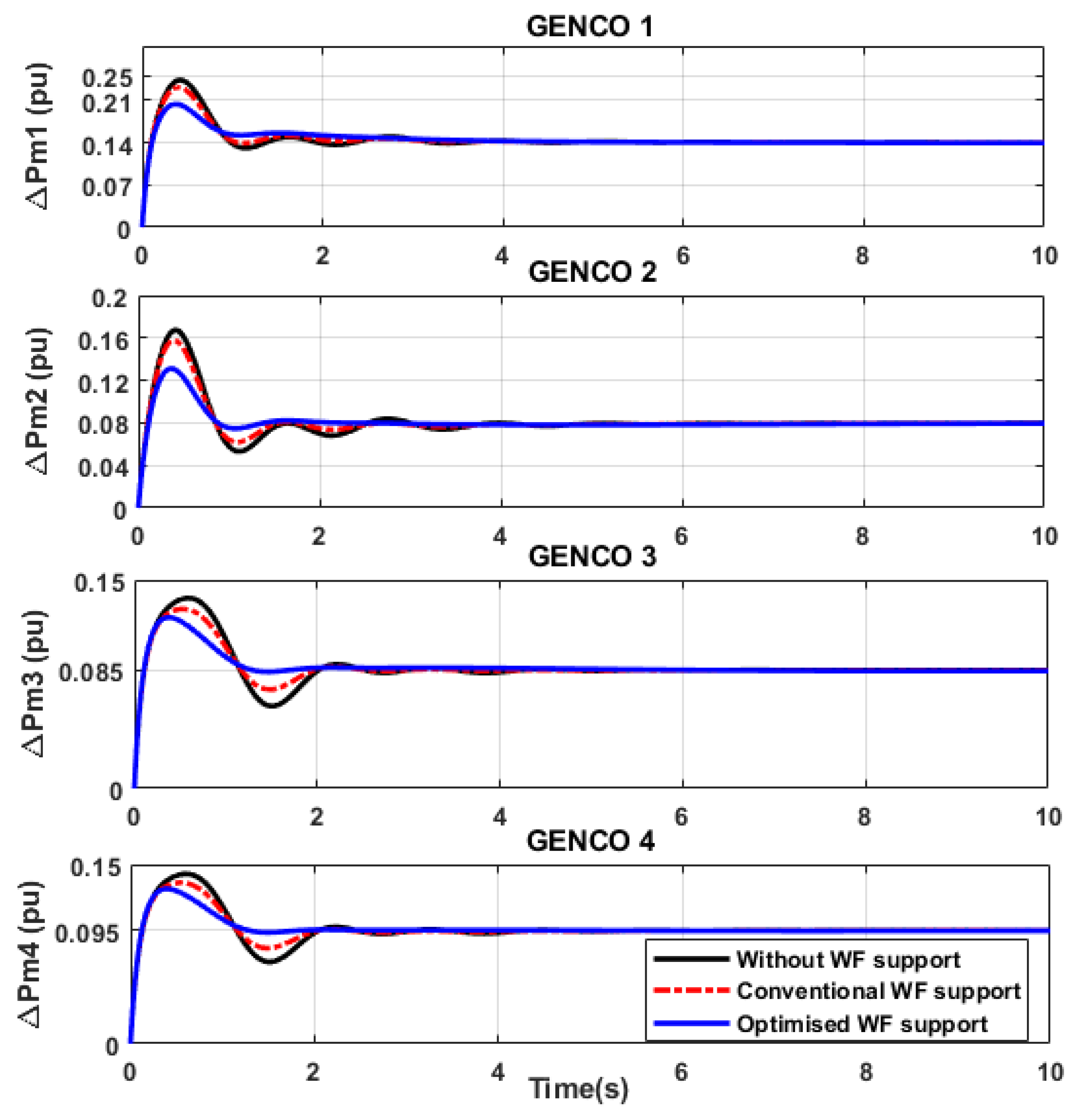
5.2.1. Scenario 1: Poolco Transaction

In a Poolco based contraction, the GENCOs participate in the frequency response control of their own control area only. In this scenario, the load demand variations of DISCO1 and DISCO2 are provided by GENCO1 and GENCO2, while the load demand variations of DISCO3 and DISCO4 are provided by GENCO3 and GENCO4. For a total load demand variation of 0.2 pu in each area, DISCO1 and DISCO2 demands are equal from GENCO1 and GENCO2, while DISCO3 and DISCO4 demands are equal from GENCO3 and GENCO4. The CPM for a Poolco based contract between the GENCOs and DISCOs used in this study is given by:
C P M = 0.5 0.5 0 0 0.5 0.5 0 0 0 0 0.5 0.5 0 0 0.5 0.5
Figure 11, Figure 12 and Figure 13 show the response of the system following a Poolco transaction.
Figure 11 represents the plot of frequency deviations in both area. It can be observed that the amplitudes of the first undershoot and overshoot are highest when there is no frequency support provided by the wind farm. With the wind farm providing support using a conventional strategy, the undershoots and overshoots are reduced by 15% and 24%, respectively, for Area 1. Using the proposed control strategy, the deviations are quickly reduced to zero steady-state with minimal oscillations in both areas. In the steady-state, the power generated by the GENCOs must match the demand of the DISCOs in contract with them. From Equation (17), the power generated by each GENCO for the respective DISCOs in contract with it can be calculated from
Δ P m 1 = Δ P m 2 = Δ P m 3 = Δ P m 4 = 0.5 × 0.1 + 0.5 × 0.1 + 0 + 0 = 0.1 pu
Figure 12 shows the various changes in active power generated by the GENCOs due to the load demand variations. The new steady-state value of each GENCO is the amount of contracted demand from the DISCOs in its area. It can be observed that the participation of wind farms in frequency control can reduce the amount of transient power needed by the GENCOs to reach the new steady-state values. By using the ABC algorithm for optimal control, the wind farm is capable of providing active power, thereby reducing the amplitude of the transient power provided by the GENCOs. It can be observed that overshoots were reduced by 16%, 14.3%, 16%, and 13.3% in the GENCOs when compared to the conventional control strategy.
Since there is no exchange of power between the areas, the scheduled tie line power flow will be zero as defined by Equation (10), so that
Δ P t i e s c h = 0 pu
However, tie line perturbations will occur when there is load demand variation due to interconnection, as shown in Figure 13.
It is generally observed that the proposed optimized controller helps the system to reach a faster settling time, with the system experiencing damping, which suppresses the oscillation, thereby providing a better dynamic response.

5.2.2. Scenario 2: Bilateral Transaction

In bilateral based transactions, DISCOs can be in contract with any GENCO within or outside their own areas; i.e., GENCOs in Area 1 can transfer power to DISCOs in Area 2 and vice versa. Therefore, inter-area exchange of power via the tie lines can be scheduled at a non-zero steady-state value. In this study, each DISCO demands 0.1 pu power from the GENCOs in both areas, as defined by the CPM below:
C P M = 0.5 0.4 0.5 0 0.2 0.1 0 0.5 0.15 0.3 0.4 0 0.15 0.2 0.1 0.5
The non-diagonal elements of the matrix correspond to the contract of a DISCO in one area with a GENCO in another area. Figure 14, Figure 15 and Figure 16 show the response of the system as a result of bilateral transaction. Figure 14 shows the frequency deviation in Areas 1 and 2. It can be seen that the peak undershoot and overshoot are high when there is no support from the wind farms. When the wind farms participate in frequency control using the conventional control, the undershoot and overshoot are reduced by 15% and 18% in Area 1 and 13% and 50% in Area 2, respectively. A further reduction is noticed when the gain of the controller is optimized using the ABC algorithm. The oscillations are suppressed and the system frequency deviation settles faster to zero in the steady-state condition.
From Equation (16), the change power generated by each GENCO in the bilateral transaction scenario can be calculated from
Δ P m 1 = 0.5 × 0.1 + 0.4 × 0.1 + 0.5 × 0.1 + 0 = 0.14 pu Δ P m 2 = 0.2 × 0.1 + 0.1 × 0.1 + 0 + 0.5 × 0.1 = 0.08 pu Δ P m 3 = 0.15 × 0.1 + 0.3 × 0.1 + 0.4 × 0.1 + 0 = 0.085 pu Δ P m 4 = 0.15 × 0.1 + 0.2 × 0.1 + 0.1 × 0.1 + 0.5 × 0.1 = 0.095 pu
The change in power generated by each GENCO is presented in Figure 15. It can be observed that, without the wind farm support, there is increased transient power generation by the GENCOs;, this deviation is reduced when there is support from the wind farm by providing active power for a short time. The effect of wind farm participation is largely noticed when the optimized derivative control is applied. This results in over 20% reduction in transient power from the GENCOs when the proposed strategy is implemented.
The scheduled tie line power flow is shown in Figure 16. This illustrates the exchange of power between both areas at steady-state. This can be calculated using
Δ P tiesch = [ 0.5 × 0.1 + 0 + 0 + 0.5 × 0.1 ] [ 0.15 × 0.1 + 0.3 × 0.1 + 0.15 × 0.1 + 0.2 × 0.1 ] = 0.1 0.08 = 0.02 pu

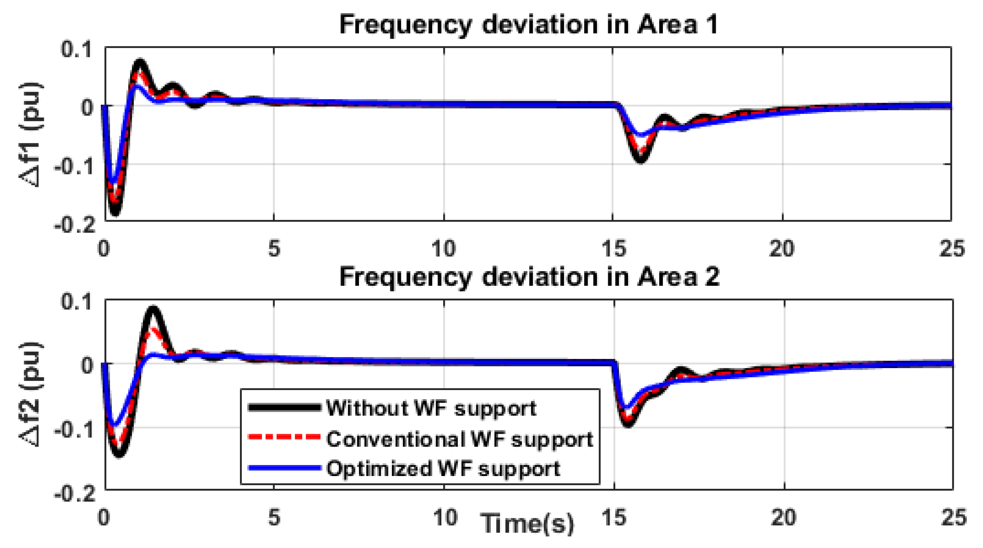
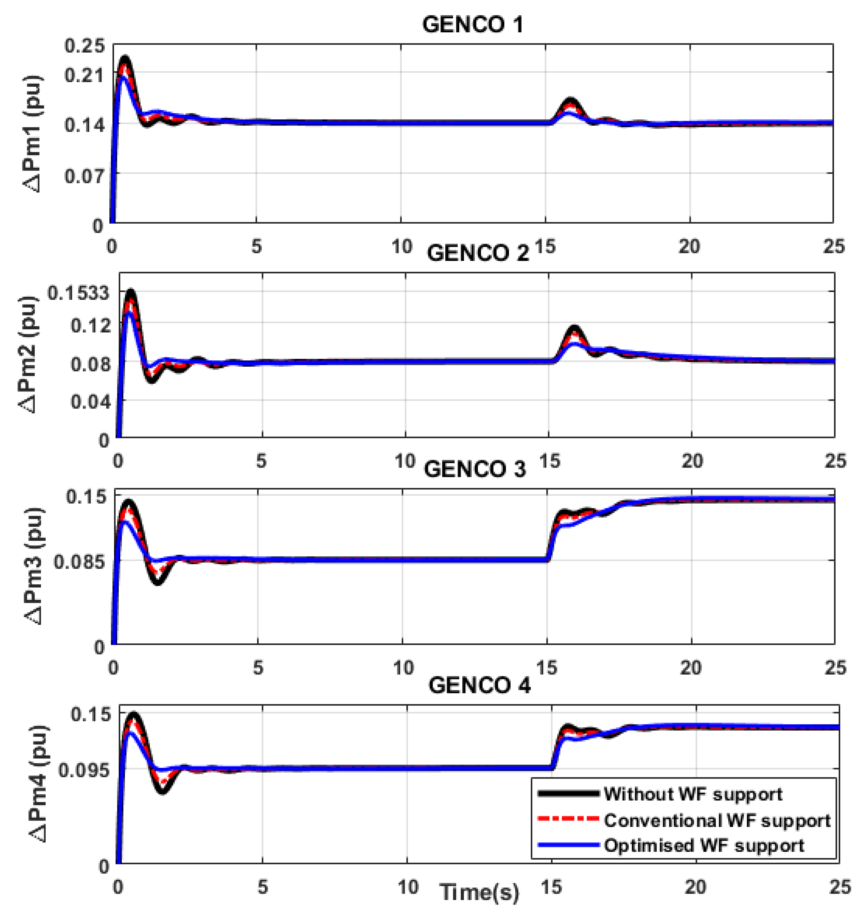
5.2.3. Scenario 3: Contract Violation

At times, DISCOs may demand more power than that specified in the contract. This extra variation is usually not contracted to any GENCO. When this happens, only GENCOs in the affected area can respond to the excess demand variations from the DISCO. The excess demand variation is always regarded as a local load demand variation. Modifying Scenario 2 (bilateral transaction) with an extra demand variation of 0.1 pu from DISCOs in Area 2 at 15 s, the CPM in Scenario 2 remains the same.
Beginning the analysis from 15 s in Figure 17, Figure 18 and Figure 19, the effect of the un-contracted load demand variation in Area 2 can be observed. From the frequency deviation plots shown in Figure 17, it can be seen that the extra load demand variation in Area 2 causes frequency dips in Areas 1 and 2 due to interconnection. The oscillations associated with the system without wind farm support are damped when the wind farms participate in frequency control; however, the proposed optimized controller has a better damping response than the conventional control strategy.
In this transaction, the change in power generation due to un-contracted variation is the responsibility of the GENCOs in that area; that is, the GENCOs in other areas return to the initial steady-state values after participating in the frequency control.
In Figure 18, the change in power generated by GENCO1 and GENCO2 remains the same; i.e., Δ P m 1 = 0.14 pu and Δ P m 2 = 0.08 pu. However, there are new steady-state values for GENCO3 and GENCO4. The changes after 15 s can be calculated using:
Δ P m 3 = 0.085 + 0.5 0.1 = 0.135 pu Δ P m 4 = 0.095 + 0.5 0.1 = 0.145 pu
The scheduled tie-line power flow remains unchanged because only the GENCOs in Area 2 supply the extra demand, as shown in Figure 19.

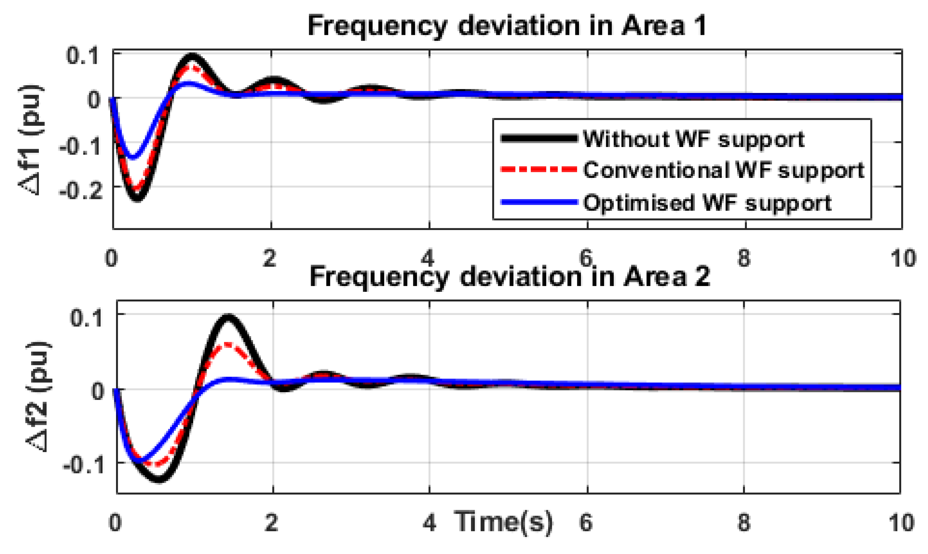
5.2.4. Scenario 4: Wind Power Fluctuation

Since wind power is largely dependent on wind speed, which is usually intermittent, it is expected that the contribution of wind farms in frequency response control will be limited. In this work, it is assumed that the de-loading margin is available in all range of wind speeds and the short-term support lasts for a fraction of second to few seconds. To test the robustness of the proposed control strategy, during wind power fluctuation, as shown in Figure 20, a change in load demand of 0.15 pu in Area 1 is simulated at 5 s.
In Figure 21, the frequency deviations in both areas of the system is presented for cases where the wind farms support in frequency stability using the conventional tuning method (dashed blue) and ABC tuning method (red). It is observed that the proposed tuning method provides better damping characteristics and reduced frequency excursions. It is pertinent to point out that the control approach proposed in this work can be extended to energy storage systems to provide mid- and long-term frequency support to power systems.

6. Conclusions

In this study, the artificial bee colony algorithm was used in the implementation of a virtual inertia control strategy. This involves the formulation, development, and simulation of a system model that can be used in traditional power systems and can be extended to modern power systems with renewable energy penetration and power system deregulation. This optimization algorithm was used to investigate the positive impact that renewable energy has on the network with respect to frequency control. The heuristic method is used to optimally tune the gain of the virtual inertia control scheme that is proposed to reduce the frequency transient deviations in a restructured power system environment. The control strategy was tested in a two-area system having conventional generation, wind power plants, and parallel ac/dc links to model a simple modern power system. Three transaction scenarios (Poolco, bilateral, and contract violation) were implemented to show the robustness of the proposed control strategy. It is generally observed that peak overshoots and undershoots, settling time, and oscillations of the system were greatly reduced. In addition, the overall dynamic performance and stability of the system are improved. The proposed strategy can be applied to expanded power systems that include more interconnected areas with additional generating plants such as solar, geothermal, ocean, and tidal power plants.

Author Contributions

A.O.A. proposed the methodology and wrote the first draft of the paper; D.G.D. edited and reviewed the second draft of the paper; R.P.C. validated the mathematical model of the paper; and E.E.O. provided software support. All authors have read and agreed to the published version of the manuscript.

Funding

This research was funded by the Royal Academy of Engineering, under the UK Newton Fund scheme, grant number IAPP161758.

Acknowledgments

The authors acknowledge Eskom’s EPPEI Specialization Center of HVDC and FACTS, University of KwaZulu-Natal, South Africa for providing research facilities.

Conflicts of Interest

The authors declare no conflict of interest.

Abbreviations

The following abbreviations are used in this manuscript
ABCArtificial bee Colony
ACEArea control error
ACOAnt colony optimization
AGCAutomatic gain control
CPMContract participation matrix
DISCODistribution company
DEDifferential Evolution
DFIGDoubly fed induction generator
GENCOGeneration company
GSCGris side converter
HVACHigh voltage alternating current
HVDCHigh voltage direct current
ISOIndependent system operator
LFCLoad frequency control
MPPTMaximum power point tracking
MSCMachine side converter
NPNectar position
PSOParticle swarm optimization
REPRenewable energy plant
VSGVirtual synchronous generator
WECSWind energy conversion system

Appendix A. Simulation Parameters

Table A1. System model parameters.
ParameterArea 1 ( i = 1 , 2 )Area 2 ( i = 3 , 4 )
Area participation factor, apf0.5, 0.50.6, 0.4
Turbine time constant, T t i (s)0.32, 0.30.3, 0.3
Governor time constant, T g i (s)0.06, 0.080.06, 0.07
Droop constant, R i (Hz/p.u MW)2.4, 2.52.5, 2.7
Damping coefficient, D (p.u MW/Hz)0.00980.0098
System inertia constant, H (p.u MWs)0.0980.1225
Frequency bias factor, β i (p.u MW/Hz)0.4250.396
Synchronizing coefficient, T 12 0.245
Area control error gain, K i 0.70.7
Area capacity ratio, α 12 -1
Wind turbine time constant, T w t (s)1.51.5
HVDC time constant, T d c (s)0.2

Appendix B. State Matrix

A = A 11 A 12 A 21 A 22
A 11 = D 1 2 H 1 0 1 2 H 1 1 2 H 1 0 0 0 0 D 2 2 H 2 0 0 1 2 H 2 1 2 H 2 0 0 0 0 1 T t 1 0 0 0 1 T t 1 0 0 0 0 1 T t 2 0 0 0 1 T t 2 0 0 0 0 1 T t 3 0 0 0 0 0 0 0 0 1 T t 4 0 0 1 R 1 T g 1 0 0 0 0 0 1 T g 1 0 1 R 2 T g 2 0 0 0 0 0 0 1 T g 2
A 12 = 0 0 0 0 1 2 H 1 1 2 H 1 1 2 H 1 0 0 0 0 0 α 12 2 H 2 α 12 2 H 2 0 1 2 H 2 0 0 0 0 0 0 0 0 0 0 0 0 0 0 0 0 1 T t 3 0 0 0 0 0 0 0 0 1 T t 4 0 0 0 0 0 0 0 0 a p f 1 T g 1 0 0 0 0 0 0 0 a p f 2 T g 2 0 0 0 0 0
A 21 = 0 1 R 3 T g 3 0 0 0 0 0 0 0 1 R 4 T g 4 0 0 0 0 0 0 β 1 K 1 0 0 0 0 0 0 0 0 β 2 K 2 0 0 0 0 0 0 2 π T 12 2 π T 12 0 0 0 0 0 0 K d c T d c K d c T d c 0 0 0 0 0 0 D 1 K w 1 2 H 1 T w 1 0 K w 1 2 H 1 T w 1 K w 1 2 H 1 T w 1 0 0 0 0 0 D 2 K w 2 2 H 2 T w 2 0 0 K w 2 2 H 2 T w 2 K w 2 2 H 2 T w 2 0 0
A 22 = 1 T g 3 0 0 a p f 3 T g 3 0 0 0 0 0 1 T g 4 0 a p f 4 T g 4 0 0 0 0 0 0 0 0 K 1 K 1 0 0 0 0 0 0 α 12 K 2 α 12 K 2 0 0 0 0 0 0 0 0 0 0 0 0 0 0 0 1 T d c 0 0 0 0 0 0 K w 1 2 H 1 T w 1 K w 1 2 H 1 T w 1 K w 1 2 H 1 T w 1 1 T w 1 0 0 0 0 0 α 12 K w 2 2 H 2 T w 2 α 12 K w 2 2 H 2 T w 2 0 K w 2 2 H 2 T w 2 1 T w 2

References

  1. Rakhshani, E.; Rodriguez, P. Active power and frequency control considering large-scale RES. In Large Scale Renewable Power Generation: Advances in Technologies for Generation, Transmission and Storage; Springer: Singapore, 2014; pp. 233–271. [Google Scholar] [CrossRef]
  2. Aluko, A.O. Modelling and performance analysis of doubly fed induction generator wind farm. Master’s Thesis, Durban University of Technology, Durban, South Africa, 2018. [Google Scholar]
  3. Aluko, A.O.; Akindeji, K. Performance analysis of grid connected scig and dfig based windfarm. In Proceedings of the 26th South African Universities Power Engineering Conference (SAUPEC), Gauteng, South Africa, 24–26 January 2018; pp. 20–25. [Google Scholar]
  4. Aluko, A.O.; Akindeji, K. Mitigation of Low Voltage Contingency of Doubly fed Induction Generator Wind farm using Static Synchronous Compensator in South Africa. In Proceedings of the IEEE PES/IAS PowerAfrica, Cape Town, South Africa, 28–29 June 2018; pp. 13–18. [Google Scholar]
  5. Lai, L.L. Power System Restructuring and Deregulation: Trading, Performance and Information Technology; John Wiley & Sons: Hoboken, NJ, USA, 2001. [Google Scholar]
  6. Bevrani, H. Robust Power System Frequency Control, 2nd ed.; Springer: Cham, Switzerland, 2014. [Google Scholar]
  7. Arya, Y. AGC of two-area electric power systems using optimized fuzzy PID with filter plus double integral controller. J. Frankl. Inst. 2018, 355, 4583–4617. [Google Scholar] [CrossRef]
  8. Ashmole, P.; Battlebury, D.; Bowdler, R. Power-system model for large frequency disturbances. Proc. Inst. Electr. Eng. (IET) 1974, 121, 601–608. [Google Scholar] [CrossRef]
  9. Pan, C.T.; Liaw, C.M. An adaptive controller for power system load-frequency control. IEEE Trans. Power Syst. 1989, 4, 122–128. [Google Scholar] [CrossRef]
  10. Rakhshani, E.; Rouzbehi, K.; Sadeh, S. A new combined model for simulation of mutual effects between LFC and AVR loops. In Proceedings of the 2009 IEEE Asia-Pacific Power and Energy Engineering Conference, Wuhan, China, 28–30 March 2009; pp. 1–5. [Google Scholar]
  11. Doolla, S.; Bhatti, T. Load frequency control of an isolated small-hydro power plant with reduced dump load. IEEE Trans. Power Syst. 2006, 21, 1912–1919. [Google Scholar] [CrossRef]
  12. Kusic, G.; Sutterfield, J.; Caprez, A.; Haneline, J.; Bergman, B. Automatic generation control for hydro systems. IEEE Trans. Energy Convers. 1988, 3, 33–39. [Google Scholar] [CrossRef]
  13. Foord, T. Step response of a governed hydrogenerator. Proc. Inst. of Electr. Eng. (IET) 1978, 125, 1247–1248. [Google Scholar] [CrossRef]
  14. Concordia, C.; Kirchmayer, L. Tie-line power and frequency control of electric power systems [includes discussion]. Trans. Am. Inst. Electr. Eng. Part III Power Appar. Syst. 1953, 72, 562–572. [Google Scholar] [CrossRef]
  15. Concordia, C.; Kirchmayer, L. Tie-Line Power and Frequency Control of Electric Power Systems-Part II [includes discussion]. Trans. Am. Inst. Electr. Eng. Part III Power Appar. Syst. 1954, 73, 133–146. [Google Scholar] [CrossRef]
  16. Kocaarslan, I.; Çam, E. Fuzzy logic controller in interconnected electrical power systems for load-frequency control. Int. J. Electr. Power Energy Syst. 2005, 27, 542–549. [Google Scholar] [CrossRef]
  17. Hore, D. An analysis of two area load frequency control with different types of feedback controllers. Int. J. Eng. Res. Technol 2014, 3, 922–925. [Google Scholar]
  18. Kothari, M.; Nanda, J.; Kothari, D.; Das, D. Discrete-mode automatic generation control of a two-area reheat thermal system with new area control error. IEEE Trans. Power Syst. 1989, 4, 730–738. [Google Scholar] [CrossRef]
  19. Verma, R.; Pal, S.; Sathans. Intelligent automatic generation control of two-area hydrothermal power system using ANN and fuzzy logic. In Proceedings of the 2013 IEEE International Conference on Communication Systems and Network Technologies, Gwalior, India, 6–8 April 2013; pp. 552–556. [Google Scholar]
  20. Saikia, L.C.; Bharali, A.; Dixit, O.; Malakar, T.; Sharma, B.; Kouli, S. Automatic generation control of multi-area hydro system using classical controllers. In Proceedings of the 2012 1st International Conference on Power and Energy in NERIST (ICPEN), Nirjuli, India, 28–29 December 2012; pp. 1–6. [Google Scholar]
  21. Bevrani, H.; Daneshfar, F.; Daneshmand, P.R. Intelligent automatic generation control: Multi-agent Bayesian networks approach. In Proceedings of the 2010 IEEE International Symposium on Intelligent Control, Yokohama, Japan, 8–10 September 2010; pp. 773–778. [Google Scholar]
  22. Yousef, H.A.; Khalfan, A.K.; Albadi, M.H.; Hosseinzadeh, N. Load frequency control of a multi-area power system: An adaptive fuzzy logic approach. IEEE Trans. Power Syst. 2014, 29, 1822–1830. [Google Scholar] [CrossRef]
  23. Adaryani, M.R.; Afrakhte, H. NARMA-L2 controller for three-area load frequency control. In Proceedings of the IEEE 2011 19th Iranian Conference on Electrical Engineering, Tehran, Iran, 17–19 May 2011; pp. 1–6. [Google Scholar]
  24. Shiroei, M.; Toulabi, M.R.; Ranjbar, A.M. Robust multivariable predictive based load frequency control considering generation rate constraint. Int. J. Electr. Power Energy Syst. 2013, 46, 405–413. [Google Scholar] [CrossRef]
  25. Jagatheesan, K.; Anand, B.; Samanta, S.; Dey, N.; Santhi, V.; Ashour, A.S.; Balas, V.E. Application of flower pollination algorithm in load frequency control of multi-area interconnected power system with nonlinearity. Neural Comput. Appl. 2017, 28, 475–488. [Google Scholar] [CrossRef]
  26. Prakash, S.; Sinha, S.K. Four area Load Frequency Control of interconnected hydro-thermal power system by Intelligent PID control technique. In Proceedings of the 2012 Students Conference on Engineering and Systems, Allahabad, India, 16–18 March 2012; pp. 1–6. [Google Scholar]
  27. Flourentzou, N.; Agelidis, V.G.; Demetriades, G.D. VSC-based HVDC power transmission systems: An overview. IEEE Trans. Power Electron. 2009, 24, 592–602. [Google Scholar] [CrossRef]
  28. Al-Haiki, Z.E.; Shaikh-Nasser, A.N. Power transmission to distant offshore facilities. IEEE Trans. Ind. Appl. 2011, 47, 1180–1183. [Google Scholar] [CrossRef]
  29. Gemmell, B.; Dorn, J.; Retzmann, D.; Soerangr, D. Prospects of multilevel VSC technologies for power transmission. In Proceedings of the 2008 IEEE/PES Transmission and Distribution Conference and Exposition, Chicago, IL, USA, 21–24 April 2008; pp. 1–16. [Google Scholar]
  30. Du, C.; Agneholm, E.; Olsson, G. Use of VSC-HVDC for industrial systems having onsite generation with frequency control. IEEE Trans. Power Deliv. 2008, 23, 2233–2240. [Google Scholar] [CrossRef]
  31. Padiyar, K. FACTS Controllers in Power Transmission and Distribution; New Age International: New Delhi, India, 2007. [Google Scholar]
  32. Du, C.; Agneholm, E.; Olsson, G. Comparison of different frequency controllers for a VSC-HVDC supplied system. IEEE Trans. Power Deliv. 2008, 23, 2224–2232. [Google Scholar] [CrossRef]
  33. Ngamroo, I. A stabilization of frequency oscillations using a power modulation control of HVDC link in a parallel AC-DC interconnected system. In Proceedings of the Power Conversion Conference-Osaka 2002 (Cat. No. 02TH8579), Osaka, Japan, 2–5 April 2002; Volume 3, pp. 1405–1410. [Google Scholar]
  34. Bevrani, H. Decentralized Robust Load-frequency Control Synthesis in Restructured Power Systems. Ph.D. Thesis, Osaka University, Osaka, Japan, 2004. [Google Scholar]
  35. Donde, V.; Pai, M.; Hiskens, I.A. Simulation and optimization in an AGC system after deregulation. IEEE Trans. Power Syst. 2001, 16, 481–489. [Google Scholar] [CrossRef]
  36. Delfino, B.; Fornari, F.; Massucco, S. Load-frequency control and inadvertent interchange evaluation in restructured power systems. IEE Proc. Gener. Transm. Distrib. 2002, 149, 607–614. [Google Scholar] [CrossRef]
  37. Sekhar, G.C.; Sahu, R.K.; Baliarsingh, A.; Panda, S. Load frequency control of power system under deregulated environment using optimal firefly algorithm. Int. J. Electr. Power Energy Syst. 2016, 74, 195–211. [Google Scholar] [CrossRef]
  38. Hosseini, S.; Etemadi, A. Adaptive neuro-fuzzy inference system based automatic generation control. Electr. Power Syst. Res. 2008, 78, 1230–1239. [Google Scholar] [CrossRef]
  39. Parmar, K.S.; Majhi, S.; Kothari, D. LFC of an interconnected power system with multi-source power generation in deregulated power environment. Int. J. Electr. Power Energy Syst. 2014, 57, 277–286. [Google Scholar] [CrossRef]
  40. Torres, M.; Lopes, L.A. An optimal virtual inertia controller to support frequency regulation in autonomous diesel power systems with high penetration of renewables. In Proceedings of the International Conference on Renewable Energies and Power Quality (ICREPQ 11), Las Palmas de Gran Canaria, Spain, 13–15 April 2011; pp. 13–15. [Google Scholar]
  41. Meng, L.; Zafar, J.; Khadem, S.K.; Collinson, A.; Murchie, K.C.; Coffele, F.; Burt, G. Fast Frequency Response from Energy Storage Systems-A Review of Grid Standards, Projects and Technical Issues. IEEE Trans. Smart Grid 2019. [Google Scholar] [CrossRef] [Green Version]
  42. Anaya-Lara, O.; Hughes, F.; Jenkins, N.; Strbac, G. Contribution of DFIG-based wind farms to power system short-term frequency regulation. IEE Proc. Gener. Transm. Distrib. 2006, 153, 164–170. [Google Scholar] [CrossRef]
  43. Li, Y.; Xu, Z.; Wong, K.P. Advanced control strategies of PMSG-based wind turbines for system inertia support. IEEE Trans. Power Syst. 2017, 32, 3027–3037. [Google Scholar] [CrossRef]
  44. Ekanayake, J.; Jenkins, N. Comparison of the response of doubly fed and fixed-speed induction generator wind turbines to changes in network frequency. IEEE Trans. Energy Convers. 2004, 19, 800–802. [Google Scholar] [CrossRef]
  45. Kanellos, F.; Hatziargyriou, N. Control of variable speed wind turbines equipped with synchronous or doubly fed induction generators supplying islanded power systems. IET Renew. Power Gener. 2009, 3, 96–108. [Google Scholar] [CrossRef]
  46. Rakhshani, E. Analysis and Control of Multi–Area HVDC Interconnected Power Systems by Using Virtual Inertia. Ph.D. Thesis, Universitat Politècnica De Catalunya, Barcelona, Spain, 2016. [Google Scholar]
  47. Aluko, A.O.; Dorrell, D.G.; Pillay-Carpanen, R.; Ojo, E.E. Frequency Control of Modern Multi-Area Power Systems Using Fuzzy Logic Controller. In Proceedings of the IEEE PES/IAS PowerAfrica, Abuja, Nigeria, 20–23 August 2019; pp. 645–649. [Google Scholar]
  48. Driesen, J.; Visscher, K. Virtual synchronous generators. In Proceedings of the IEEE Power and Energy Society General Meeting-Conversion and Delivery of Electrical Energy in the 21st Century, Pittsburgh, PA, USA, 20–24 July 2008; pp. 1–3. [Google Scholar]
  49. Tamrakar, U.; Shrestha, D.; Maharjan, M.; Bhattarai, B.; Hansen, T.; Tonkoski, R. Virtual inertia: Current trends and future directions. Appl. Sci. 2017, 7, 654. [Google Scholar] [CrossRef]
  50. Chatterjee, K. Design of dual mode PI controller for load frequency control. Int. J. Emerg. Electr. Power Syst. 2011, 11. [Google Scholar] [CrossRef]
  51. Bevrani, H.; Hiyama, T. On load–frequency regulation with time delays: design and real-time implementation. IEEE Trans. Energy Convers. 2009, 24, 292–300. [Google Scholar] [CrossRef]
  52. Vrdoljak, K.; Perić, N.; Šepac, D. Optimal distribution of load-frequency control signal to hydro power plants. In Proceedings of the 2010 IEEE International Symposium on Industrial Electronics, Bari, Italy, 4–7 July 2010; pp. 286–291. [Google Scholar]
  53. Ray, P.K.; Mohanty, S.R.; Kishor, N. Proportional–integral controller based small-signal analysis of hybrid distributed generation systems. Energy Convers. Manag. 2011, 52, 1943–1954. [Google Scholar] [CrossRef]
  54. Calovic, M. Linear regulator design for a load and frequency control. IEEE Trans. Power Appar. Syst. 1972, 6, 2271–2285. [Google Scholar] [CrossRef]
  55. Barcelo, W.R. Effect of power plant response on optimum load frequency control system design. IEEE Trans. Power Appar. Syst. 1973, 1, 254–258. [Google Scholar] [CrossRef]
  56. Bevrani, H. Robust load frequency controller in a deregulated environment: A/spl mu/-synthesis approach. In Proceedings of the 1999 IEEE International Conference on Control Applications (Cat. No. 99CH36328), Kohala Coast, HI, USA, 22–27 August 1999; Volume 1, pp. 616–621. [Google Scholar]
  57. Chaudhuri, B.; Pal, B.C.; Zolotas, A.C.; Jaimoukha, I.M.; Green, T.C. Mixed-sensitivity approach to H/sub/spl infin//control of power system oscillations employing multiple FACTS devices. IEEE Trans. Power Syst. 2003, 18, 1149–1156. [Google Scholar] [CrossRef] [Green Version]
  58. Rosyiana Fitri, I.; Kim, J.S.; Song, H. High-Gain Disturbance Observer-Based Robust Load Frequency Control of Power Systems with Multiple Areas. Energies 2017, 10, 595. [Google Scholar] [CrossRef] [Green Version]
  59. Karnavas, Y.; Papadopoulos, D. AGC for autonomous power system using combined intelligent techniques. Electr. Power Syst. Res. 2002, 62, 225–239. [Google Scholar] [CrossRef]
  60. Ibraheem; Kumar, P.; Hasan, N.; Nizamuddin. Sub-optimal automatic generation control of interconnected power system using output vector feedback control strategy. Electr. Power Compon. Syst. 2012, 40, 977–994. [Google Scholar] [CrossRef]
  61. Hasan, N.; Kumar, P.; others. Sub-optimal automatic generation control of interconnected power system using constrained feedback control strategy. Int. J. Electr. Power Energy Syst. 2012, 43, 295–303. [Google Scholar] [CrossRef]
  62. Onaolapo, A.K. Modeling and recognition of faults in smart distribution grid using machine intelligence technique. Ph.D. Thesis, Durban University of Technology, Durban, South Africa, 2018. [Google Scholar]
  63. Bhatti, T.; Ibraheem; Nizamuddin. AGC of two area power system interconnected by AC/DC links with diverse sources in each area. Int. J. Electr. Power Energy Syst. 2014, 55, 297–304. [Google Scholar]
  64. Variani, M.H.; Tomsovic, K. Distributed automatic generation control using flatness-based approach for high penetration of wind generation. IEEE Trans. Power Syst. 2013, 28, 3002–3009. [Google Scholar] [CrossRef]
  65. Safari, A.; Babaei, F.; Farrokhifar, M. A load frequency control using a PSO-based ANN for micro-grids in the presence of electric vehicles. Int. J. Ambient Energy 2019, 1–13. [Google Scholar] [CrossRef]
  66. Khooban, M.H. Secondary load frequency control of time-delay stand-alone microgrids with electric vehicles. IEEE Trans. Ind. Electron. 2017, 65, 7416–7422. [Google Scholar] [CrossRef]
  67. Xi, J.; Geng, H.; Yang, G. Adaptive VSG Control of PMSG based WECS for Grid Frequency Response. In Proceedings of the IEEE International Power Electronics and Application Conference and Exposition (PEAC), Shenzhen, China, 4–7 November 2018; pp. 1–5. [Google Scholar]
  68. Sharma, G.; Nasiruddin, I.; Niazi, K.; Bansal, R. Automatic Generation Control (AGC) of Wind Power System: An Least Squares-Support Vector Machine (LS-SVM) Radial Basis Function (RBF) Kernel Approach. Electr. Power Compon. Syst. 2018, 46, 1621–1633. [Google Scholar] [CrossRef]
  69. Sahu, R.K.; Sekhar, G.C.; Panda, S. DE optimized fuzzy PID controller with derivative filter for LFC of multi source power system in deregulated environment. Ain Shams Eng. J. 2015, 6, 511–530. [Google Scholar] [CrossRef] [Green Version]
  70. Alhelou, H.H.; Hamedani-Golshan, M.E.; Zamani, R.; Heydarian-Forushani, E.; Siano, P. Challenges and opportunities of load frequency control in conventional, modern and future smart power systems: A comprehensive review. Energies 2018, 11, 2497. [Google Scholar] [CrossRef] [Green Version]
  71. Rodriguez, P.; Candela, I.; Luna, A. Control of PV generation systems using the synchronous power controller. In Proceedings of the IEEE Energy Conversion Congress and Exposition, Denver, CO, USA, 15–19 September 2013; pp. 993–998. [Google Scholar] [CrossRef]
  72. Ayan, K.; Kılıç, U. Artificial bee colony algorithm solution for optimal reactive power flow. Appl. Soft Comput. 2012, 12, 1477–1482. [Google Scholar] [CrossRef]
  73. Karaboga, D.; Gorkemli, B.; Ozturk, C.; Karaboga, N. A comprehensive survey: artificial bee colony (ABC) algorithm and applications. Artif. Intell. Rev. 2014, 42, 21–57. [Google Scholar] [CrossRef]
  74. Sumpavakup, C.; Srikun, I.; Chusanapiputt, S. A solution to the optimal power flow using artificial bee colony algorithm. In Proceedings of the IEEE International Conference on Power System Technology, Minneapolis, MN, USA, 25–29 July 2010; pp. 1–5. [Google Scholar]
  75. Gozde, H.; Taplamacioglu, M.C.; Kocaarslan, I. Comparative performance analysis of Artificial Bee Colony algorithm in automatic generation control for interconnected reheat thermal power system. Int. J. Electr. Power Energy Syst. 2012, 42, 167–178. [Google Scholar] [CrossRef]
  76. Karaboga, D.; Akay, B. A survey: algorithms simulating bee swarm intelligence. Artif. Intell. Rev. 2009, 31, 61–85. [Google Scholar] [CrossRef]
  77. Karaboga, D.; Basturk, B. On the performance of artificial bee colony (ABC) algorithm. Appl. Soft Comput. 2008, 8, 687–697. [Google Scholar] [CrossRef]
  78. Benyoucef, A.s.; Chouder, A.; Kara, K.; Silvestre, S.; sahed, O.A. Artificial bee colony based algorithm for maximum power point tracking (MPPT) for PV systems operating under partial shaded conditions. Appl. Soft Comput. 2015, 32, 38–48. [Google Scholar] [CrossRef] [Green Version]
  79. Abu-Mouti, F.S.; El-Hawary, M.E. Optimal Distributed Generation Allocation and Sizing in Distribution Systems via Artificial Bee Colony Algorithm. IEEE Trans. Power Deliv. 2011, 26, 2090–2101. [Google Scholar] [CrossRef]
  80. Kundur, P.; Balu, N.J.; Lauby, M.G. Power System Stability and Control; McGraw-Hill: New York, NY, USA, 1994; Volume 7. [Google Scholar]
  81. Inoue, T.; Amano, H. A thermal power plant model for dynamic simulation of load frequency control. In Proceedings of the 2006 IEEE PES Power Systems Conference and Exposition, Atlanta, GA, USA, 29 October–1 November 2006; pp. 1442–1447. [Google Scholar]
  82. Bhatt, P.; Roy, R.; Ghoshal, S. Optimized multi area AGC simulation in restructured power systems. Int. J. Electr. Power Energy Syst. 2010, 32, 311–322. [Google Scholar] [CrossRef]
  83. Abraham, R.J.; Das, D.; Patra, A. Load following in a bilateral market with local controllers. Int. J. Electr. Power Energy Syst. 2011, 33, 1648–1657. [Google Scholar] [CrossRef]
  84. Tan, W.; Zhang, H.; Yu, M. Decentralized load frequency control in deregulated environments. Int. J. Electr. Power Energy Syst. 2012, 41, 16–26. [Google Scholar] [CrossRef]
  85. Sewchurran, S.; Davidson, I.E. Introduction to the South African Renewable Energy Grid Code version 2.9 requirements (Part II—Grid code technical requirements). In Proceedings of the2017 IEEE AFRICON, Cape Town, South Africa, 18–20 September 2017; pp. 1225–1230. [Google Scholar]
  86. Kerdphol, T.; Rahman, F.; Mitani, Y. Virtual inertia control application to enhance frequency stability of interconnected power systems with high renewable energy penetration. Energies 2018, 11, 981. [Google Scholar] [CrossRef] [Green Version]
  87. Al-Toma, A.S.H. Hybrid Control Schemes for Permanent Magnet Synchronous Generator Wind Turbines. Ph.D. Thesis, Brunel University London, London, UK, 2017. [Google Scholar]
  88. Karaboga, D. An Idea Based on Honey Bee Swarm for Numerical Optimization; Report; Erciyes University: Kayseri, Turkey, 2005. [Google Scholar]
  89. Karaboga, D.; Basturk, B. A powerful and efficient algorithm for numerical function optimization: artificial bee colony (ABC) algorithm. J. Glob. Optim. 2007, 39, 459–471. [Google Scholar] [CrossRef]
  90. Bao, L.; Zeng, J.C. Comparison and analysis of the selection mechanism in the artificial bee colony algorithm. In Proceedings of the IEEE Ninth International Conference on Hybrid Intelligent Systems, Shenyang, China, 12–14 August 2009; Volume 1, pp. 411–416. [Google Scholar]
  91. Burns, R. Advanced Control Engineering; Butterworth-Heinemann: Oxford, UK, 2001. [Google Scholar]
Figure 1. Classification of frequency control techniques in wind energy systems.
Energies 13 00564 g001
Figure 2. System model.
Energies 13 00564 g002
Figure 3. Frequency response model of a two area power system in a deregulated environment.
Energies 13 00564 g003
Figure 4. Dynamics of deregulation contract.
Energies 13 00564 g004
Figure 5. Frequency deviation comparison of AC and AC/DC systems.
Energies 13 00564 g005
Figure 6. Grid-connected PMSG WECS.
Energies 13 00564 g006
Figure 7. Modified control scheme of MSC.
Energies 13 00564 g007
Figure 8. Derivative control loop for WECS.
Energies 13 00564 g008
Figure 9. Flowchart of ABC optimization algorithm.
Energies 13 00564 g009
Figure 10. Eigenvalue plot of two systems.
Energies 13 00564 g010
Figure 11. Frequency deviation in a Poolco transaction.
Energies 13 00564 g011
Figure 12. Change in power generation of GENCOs in a Poolco transaction.
Energies 13 00564 g012
Figure 13. Tie line power flow in a Poolco transaction.
Energies 13 00564 g013
Figure 14. Frequency deviation in bilateral transaction.
Energies 13 00564 g014
Figure 15. Change in power generation of GENCOs in bilateral transaction.
Energies 13 00564 g015
Figure 16. Tie line power flow in bilateral transaction.
Energies 13 00564 g016
Figure 17. Frequency deviation in contract violation.
Energies 13 00564 g017
Figure 18. Active power generation of GENCOs in contract violation.
Energies 13 00564 g018
Figure 19. Tie line power flow in contract violation.
Energies 13 00564 g019
Figure 20. Wind power fluctuation.
Energies 13 00564 g020
Figure 21. Frequency deviation during wind power fluctuation.
Energies 13 00564 g021
Table 1. ABC algorithm parameters.
ParameterValue
Maximum cycle number (MCN)300
Colony size (CS)200
Number of employed bees100
Number of design variables (V)2
Limit 0.6 * CS * V
Table 2. Comparison of eigenvalues.
ModeNo WF SupportWith WF Support (Conventional)With WF Support (Optimized)
λ 1 −17.1457−17.1558−17.2131
λ 2 −17.0903−17.0886−17.1309
λ 3 −13.0917−13.0257−13.0843
λ 4 −14.6662−14.6012−14.6278
λ 5 −0.1780 + j4.7456−0.7186 + j5.2526−1.6315 + j5.2273
λ 6 −0.1780 − j4.7456−0.7186 − j5.2526−1.6315 − j5.2273
λ 7 −0.9682 + j3.0929−1.3347 + j3.0070−2.2055 + j3.2540
λ 8 −0.9682 − j3.0929−1.3347−j3.0070−2.2055 − j3.2540
λ 9 −0.4172−0.9282 + j0.6974−0.8046 + j0.8489
λ 10 −1.2326 + j0.4645−0.9282 − j0.6974−0.8046 − j0.8489
λ 11 −1.2326 − j0.4645−0.4723 + j0.1527−0.3370 + j0.2541
λ 12 −2.9151−0.4723 − j0.1527−0.3370 − j0.2541
λ 13 −3.2156−0.6382−0.5834
λ 14 −3.2314−3.0310−3.0355
λ 15 ———-−3.2264 + j0.0034−3.2258 + j0.0033
λ 16 ———-−3.2264 − j0.0034−3.2258 − j0.0033
Table 3. Comparison of total damping.
ParameterNo WF SupportWith WF Support (Conventional)With WF Support (Optimized)
Total Damping76.459078. 900882.08 37

