Thermo-Economic Analysis of a Hybrid Ejector Refrigerating System Based on a Low Grade Heat Source


Abstract
:
1. Introduction
1.1. State of the Art of Heat Driven System Technologies
1.1.1. Absorption Systems
1.1.2. ORC Coupled to Vapor Compression Cycle (VCC) Systems
1.1.3. Hybrid Ejector Systems
1.2. Aim of the Paper
- To estimate performances and costs for the typical operating conditions of a waste heat recovery hybrid ejector cycle (WHRHEC). The results of the proposed thermo-economic analysis should be useful to place the WHRHEC systems among the actual heat driven cooling technologies available on the market, in terms of two conflicting goals (performance/investment costs).
- To use the estimation of the performances and costs to evaluate the economical convenience of a waste heat recovery hybrid ejector cycle (WHRHEC) integrated to a conventional vapor compression cycle (VCC). The following economic analysis will give to the reader realistic information about the economic convenience in the use of the WHRHEC systems instead of traditional vapor compression cycles, when a certain amount of waste heat is available.
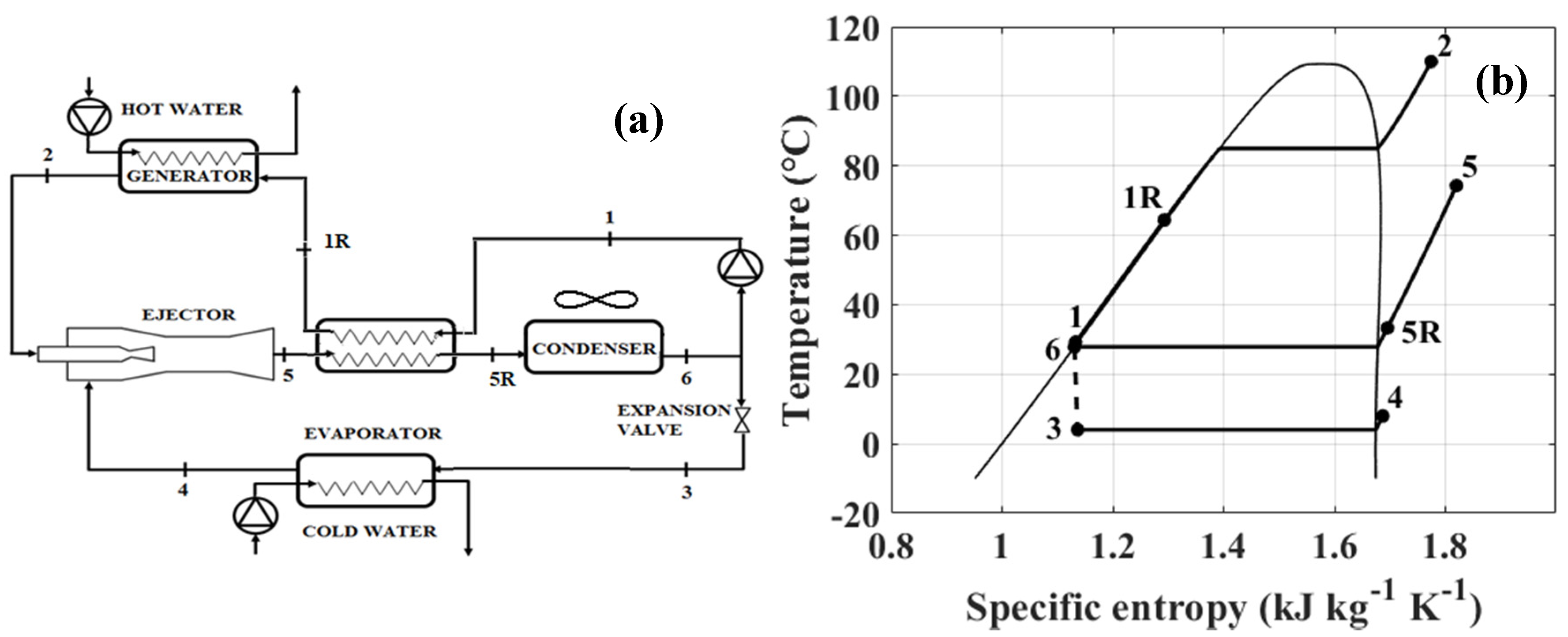
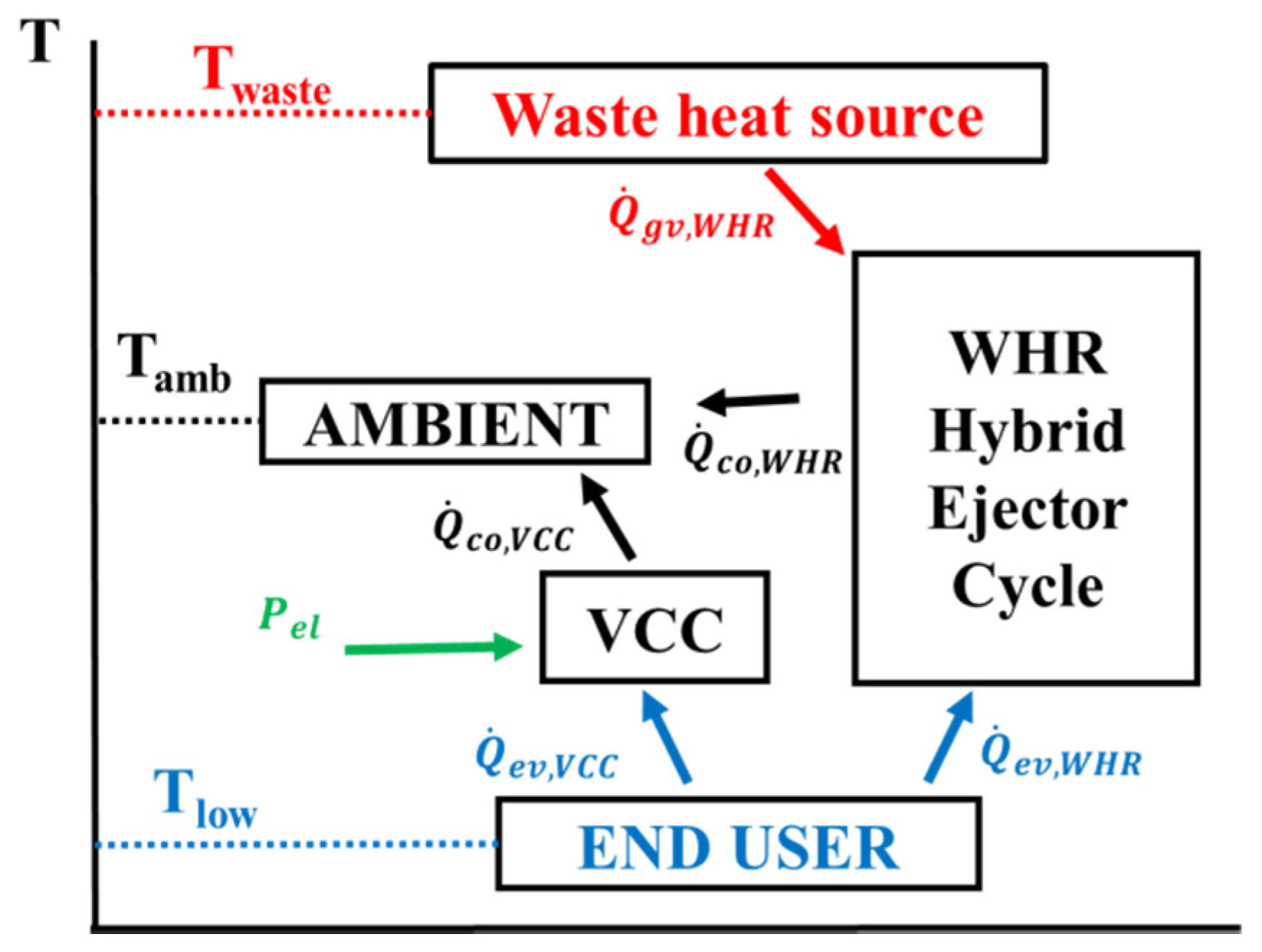
2. Hybrid Ejector Cycle: Modeling and Thermodynamic Analysis
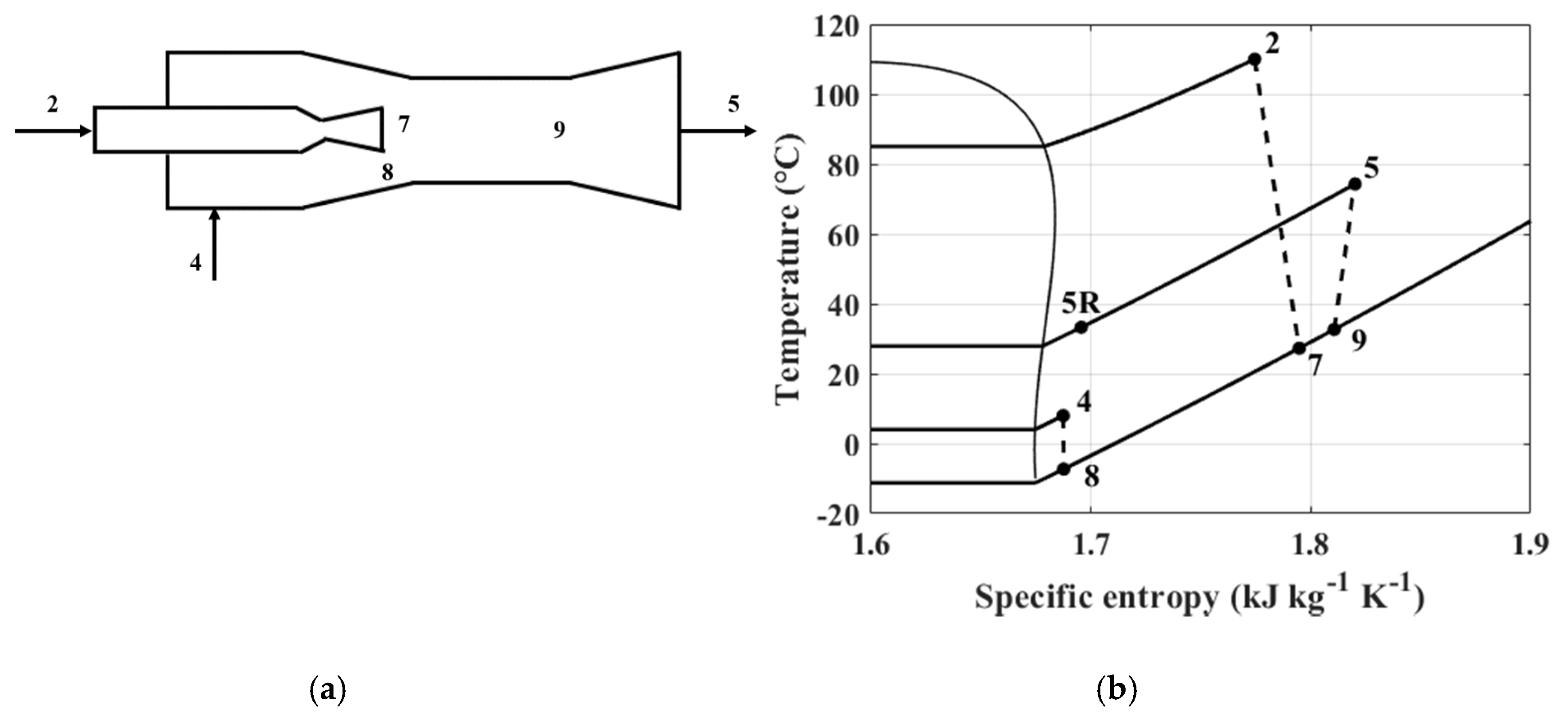
2.1. Ejector Model
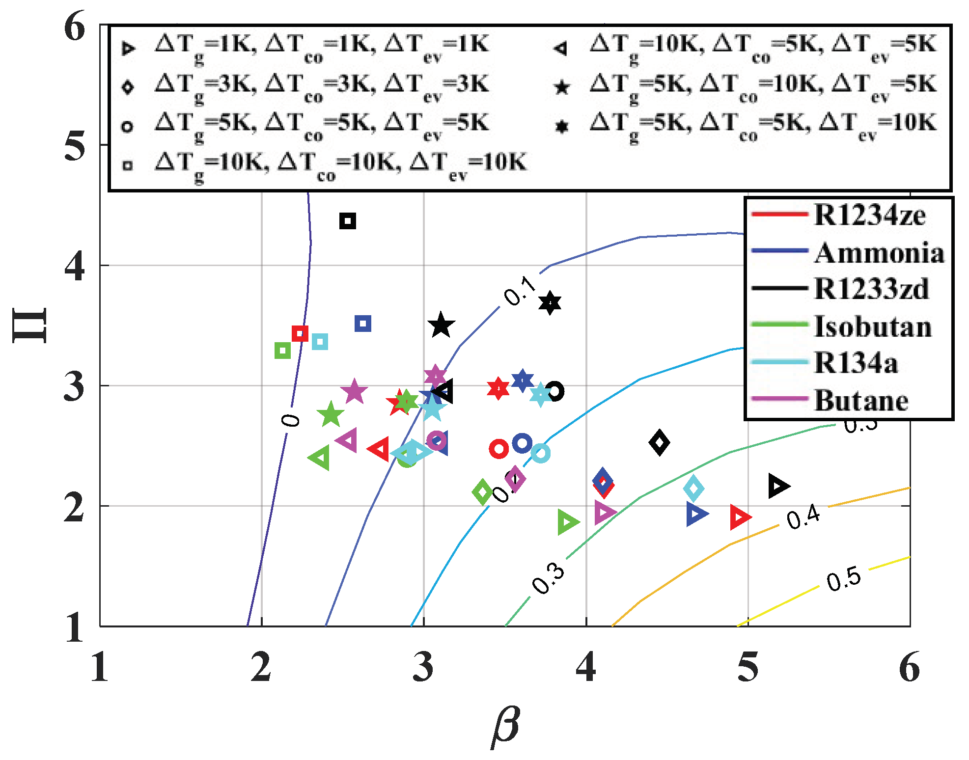
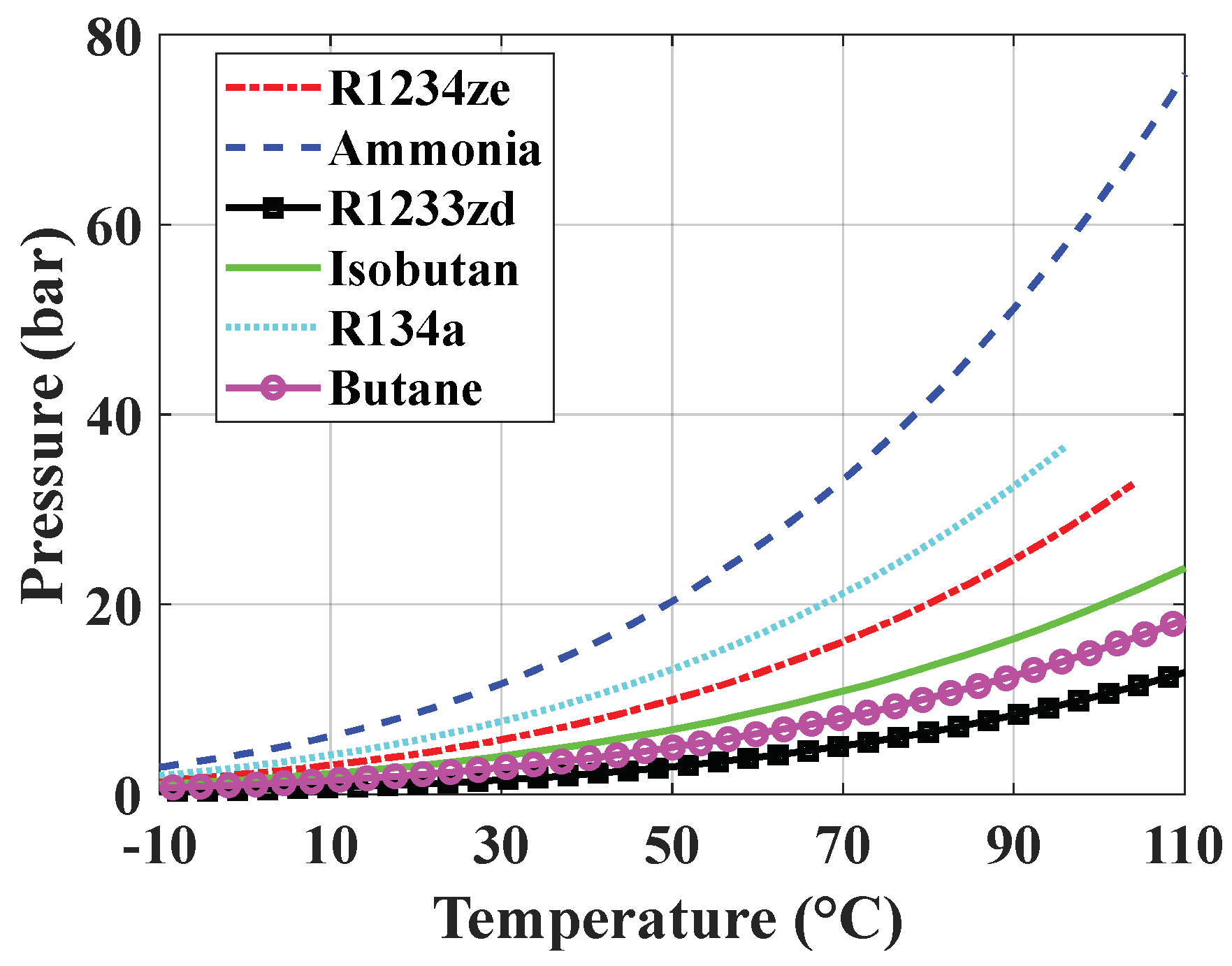
2.2. Working Fluids
- high latent heat value in the evaporator and generator temperature range to minimize the mass flow rate per unit of heat power;
- relatively high critical temperature to make the system feasible in a wide range of generator temperatures;
- not too high saturation pressure in the generator and not too low in the evaporator.
2.3. Thermodynamic Analysis: Conditions and Results
3. Thermo-Economic Analysis
3.1. Evaluation of the Heat Exchangers Surface
3.2. Cost Functions
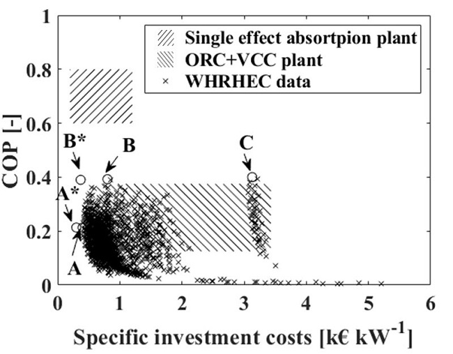
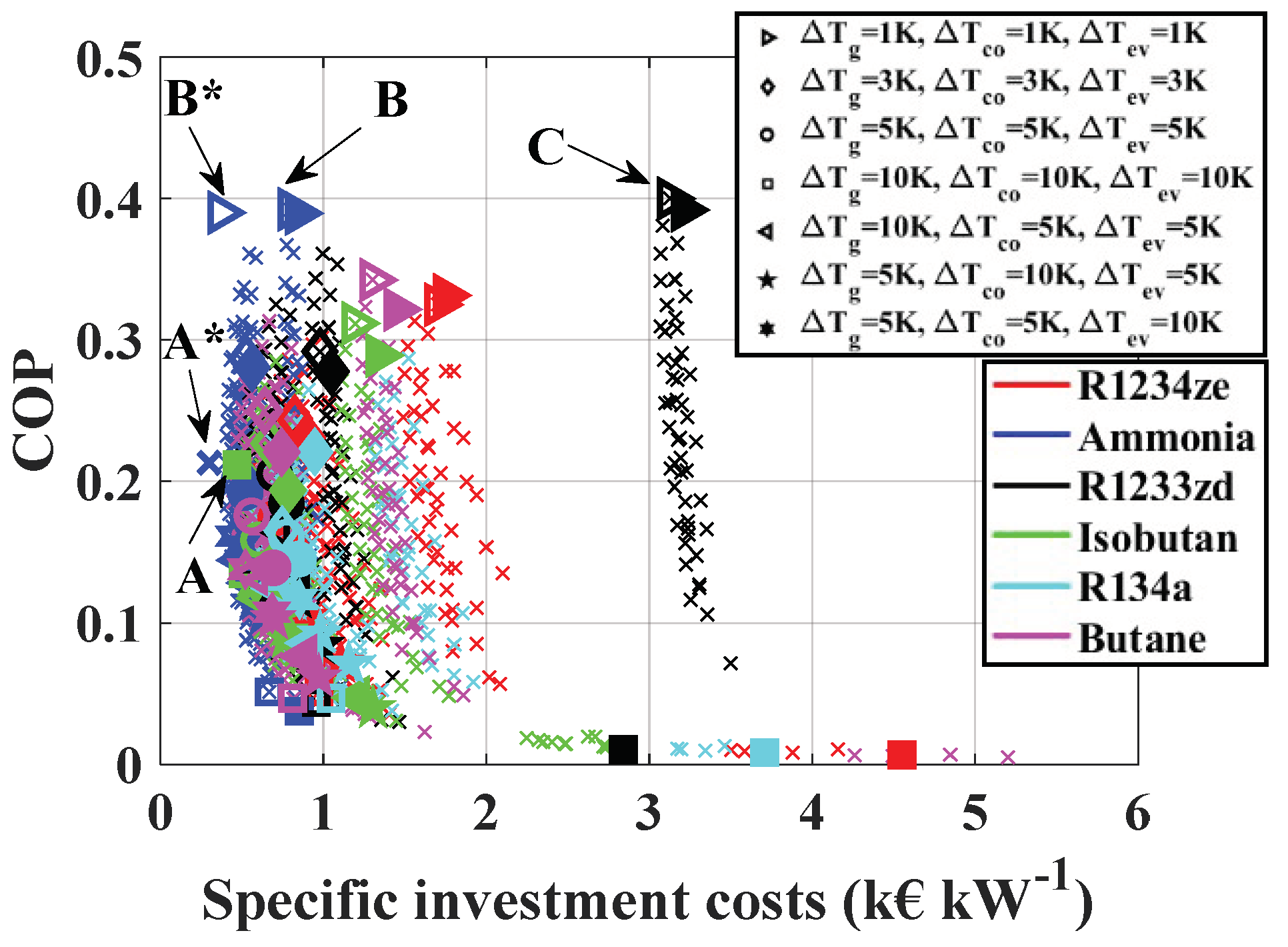
3.3. Results and Discussion
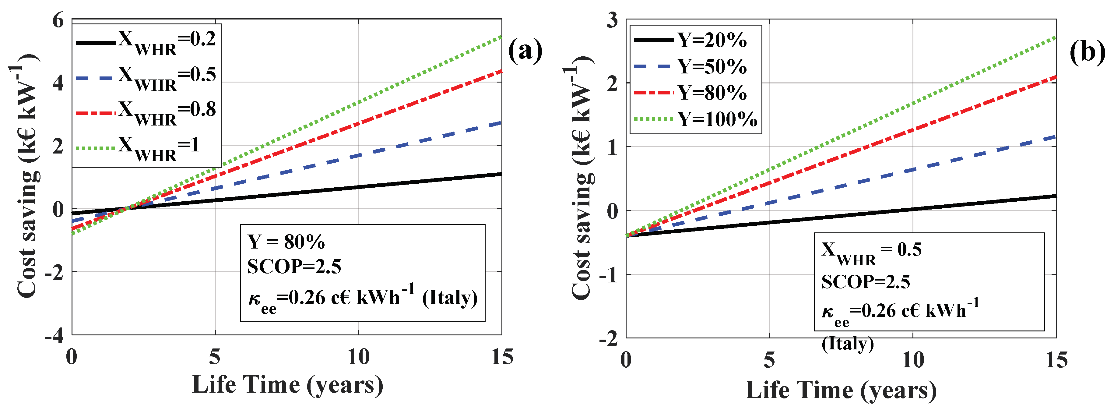
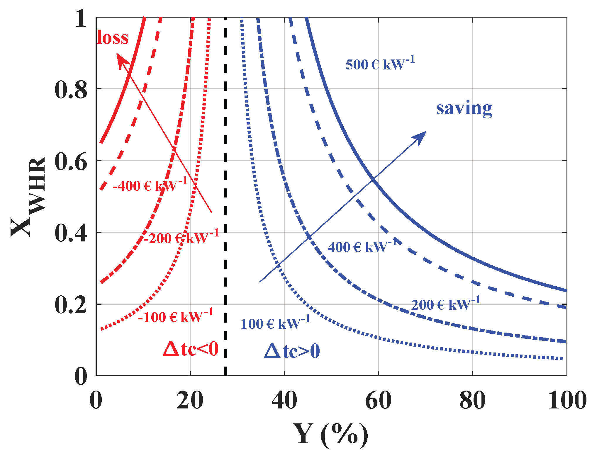
3.4. Total Costs Analysis for VCC Integrated User
4. Conclusions
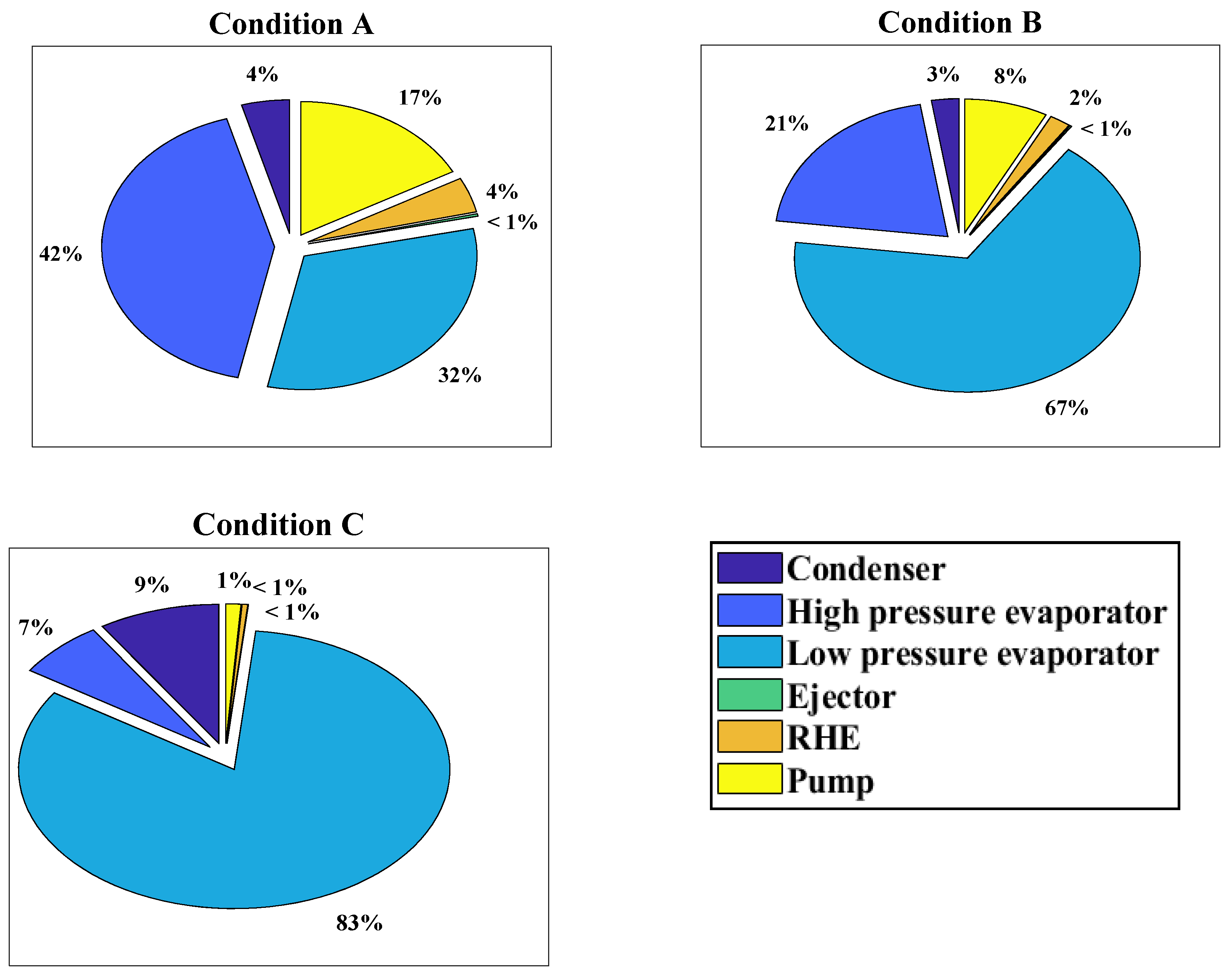
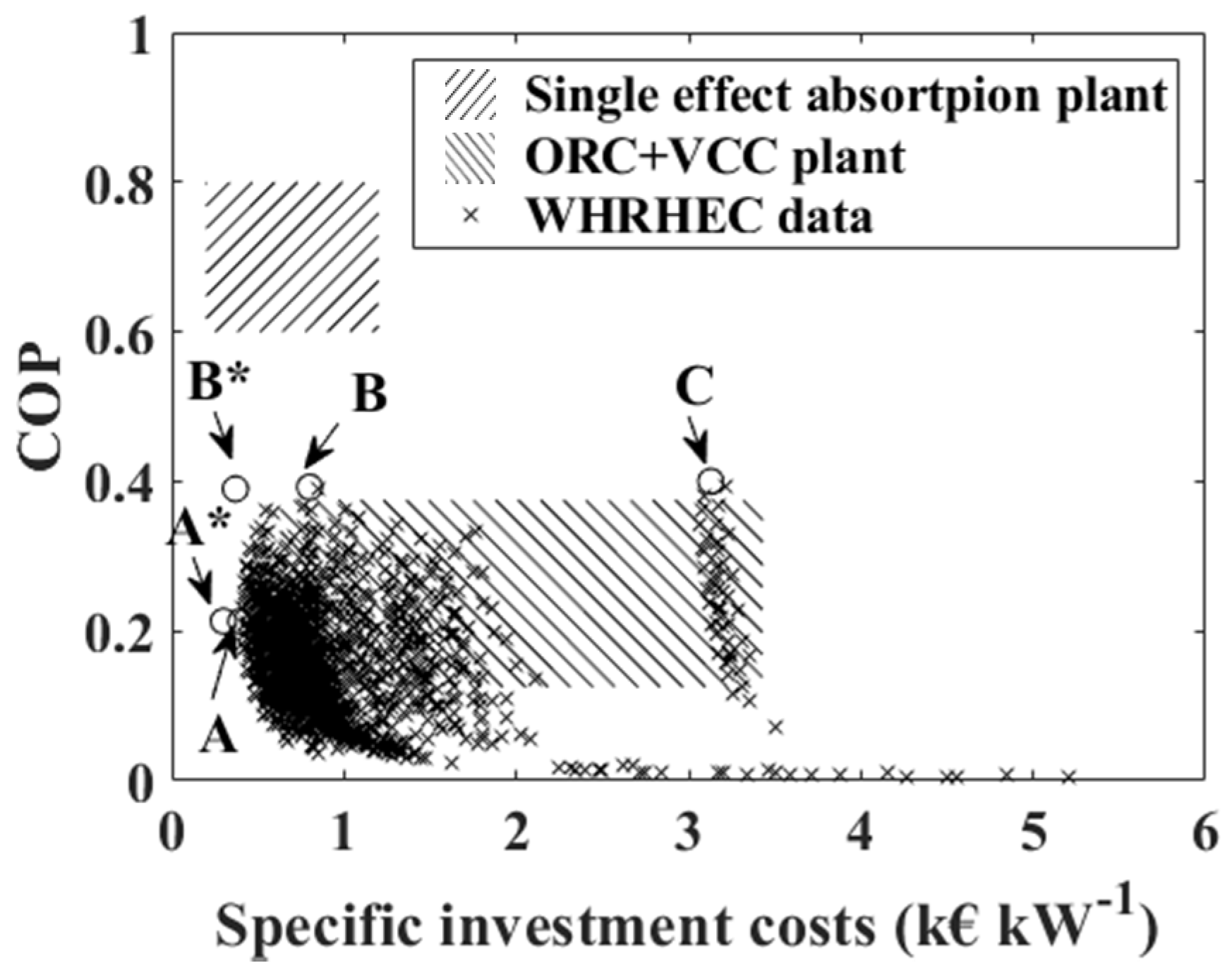
- WHRHEC solutions employing ammonia are the most performing and also economically advantageous cases, due to the ammonia high latent heat and favorable thermodynamic and transport properties during two-phase heat transfer. Moreover, the higher low-temperature evaporating pressures may allow the use of a cheaper and more compact plate heat exchanger instead of a tube and shell low-temperature evaporator, thus further reducing the set-up costs (solutions A* and B*).
- The cost-performance comparison with existing waste heat driven technologies for cooling purposes shows that the WHRHEC systems provide similar performances and lower investment costs with respect to ORC/VCC combined plants; instead WHRHEC systems give lower COP values at the same costs of single-effect absorption chillers. However, the declared performances of the consolidated technologies are related to large plant sizes and cooling loads (>100 kW), while costs of WHRHEC systems is not affected by size effects.
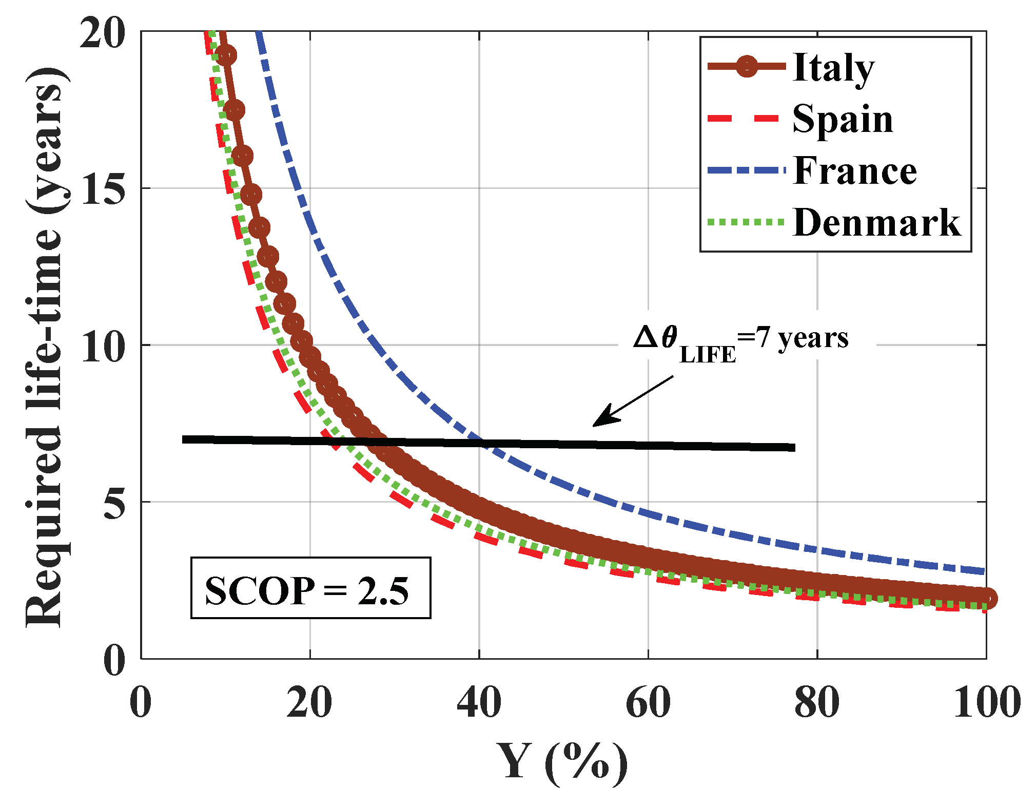
- The economic analysis has shown that a WHRHEC may be a convenient solution to be integrated with a conventional VCC system in a plant according to the specific cost of electric energy and the waste heat time availability. Specifically, for the Italian situation, by considering a total lifetime of 28,000 h (7 years and 4000 h per year of operation), the economical convenience of the WHRHEC system is reached when the waste heat exploitation overcomes approximately 7800 h (28% of the entire lifetime). Higher (lower) waste-heat availability periods are instead required where the cost of electric energy is lower (higher), as in France (40%) (as in Spain, 24% and Denmark, 26%).
Author Contributions
Funding
Conflicts of Interest
Nomenclature
| A | heat exchanger surface (m2) | Greek | |
| Ar | ejector area ratio (m2) | α | convective heat transfer coefficient (W m−2 K−1) |
| cp | specific heat at constant pressure (kJ kg−1 K−1) | β | ejector beta ratio |
| COP | coefficient of performance | Δ | difference |
| D | diameter (m) | ε | heat exchanger efficiency |
| Eel | electrical energy consumption (kJ) | η | efficiency |
| GWP | global warming potential (kgCO2eq kg−1) | θ | time |
| h | specific enthalpy (kJ kg−1) | κ | thermal conductivity [W m−1 K−1) |
| ic | specific investment costs (k€ kW−1) | κ ee | specific cost of electric energy (€ kWh−1) |
| IC | investment costs (k€) | μ | entrainment ratio |
| k | heat capacity ratio | Π | pressure lift |
| kvcc | Set-up specific cost VCC (k€ kW−1) | Subscripts | |
| kWHR | Set-up specific cost WHR (k€ kW−1) | air | related to the air |
| G | mass flux (kg s−1 m−2) | co | condenser |
| mass flow rate (kg s−1) | cold | cold side | |
| N | number of elements | cr | critical condition |
| Nu | Nusselt number | D | diffuser |
| ODP | ozone depletion potential | ev | evaporator |
| ORC | organic Rankine cycle | f | secondary fluid |
| P | pressure (bar) | fin | fin |
| Pr | Prandtl number | fluid | related to the fluid |
| heat capacity (kW) | h | hydraulic | |
| R | ideal gas constant (kJ kg−1 K−1) | hot | hot side |
| Re | Reynolds number | M | mixing chamber |
| s | tube thickness (m) | m | mixing section |
| SCOP | seasonal coefficient of performance | mat | material |
| T | temperature (K) | N | motive nozzle |
| tc | specific total costs (k€ kW−1) | nb | nucleate boiling contribution |
| TC | total costs (k€) | pf | primary flow |
| u | velocity (m s−1) | R | rank |
| U | overall heat transfer coefficient (W m−2 K−1) | ref | related to the refrigerant |
| V | volume (m3) | rhe | regenerative heat exchanger |
| VCC | vapor compression cycle | s | isentropic |
| W | power consumption (kW) | sf | secondary flow |
| WHRHEC | waste heat recovery hybrid ejector cycle | t | motive nozzle throat section |
| XWHR | fraction of the cooling load covered by the WHR plant | tp | two−phase |
| Y | fraction of the total lifetime period when the waste heat source is available | vg | vapor generator |
| WHR | waste heat recovery | ||
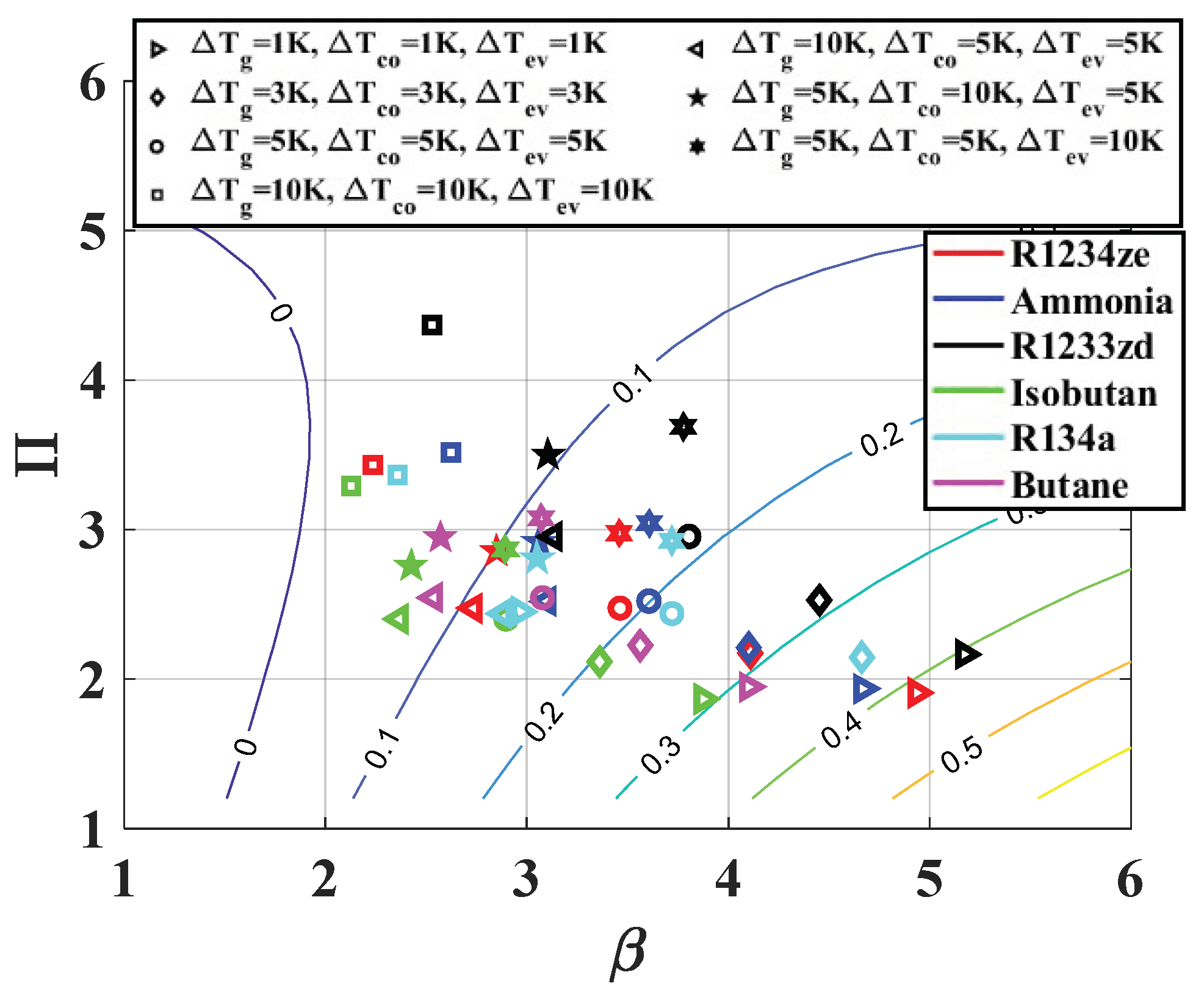
Appendix A. Thermodynamic Analysis Results

| R1234ze | ||||||||||||||
|---|---|---|---|---|---|---|---|---|---|---|---|---|---|---|
| ∆Tgv (°C) | ∆Tco (°C) | ∆Tev (°C) | Tgv (°C) | Pgv (bar) | Tco (°C) | Pco (bar) | Tev (°C) | Pev (bar) | µ (-) | Π (-) | β (-) | COP (-) | Qgv (kW) | Qco (kW) |
| 1 | 1 | 1 | 91.1 | 25.3 | 25.8 | 5.1 | 6 | 2.7 | 0.370 | 1.90 | 4.95 | 0.33 | 60.0 | 80.9 |
| 3 | 3 | 3 | 85.0 | 22.33 | 27.9 | 5.43 | 4 | 2.50 | 0.261 | 2.17 | 4.11 | 0.23 | 86.6 | 107.6 |
| 5 | 5 | 5 | 79.7 | 19.95 | 29.9 | 5.76 | 2 | 2.33 | 0.173 | 2.47 | 3.46 | 0.15 | 133.0 | 154.4 |
| 10 | 5 | 5 | 69.0 | 15.75 | 29.9 | 5.76 | 2 | 2.33 | 0.096 | 2.47 | 2.73 | 0.08 | 237.0 | 258.7 |
| 5 | 10 | 5 | 77.3 | 18.95 | 34.9 | 6.65 | 2 | 2.33 | 0.084 | 2.85 | 2.85 | 0.07 | 279.7 | 302.3 |
| 5 | 5 | 10 | 79.7 | 19.94 | 29.9 | 5.76 | −3 | 1.94 | 0.140 | 2.98 | 3.46 | 0.12 | 168.0 | 189.7 |
| 10 | 10 | 10 | 66.5 | 14.86 | 34.8 | 6.65 | −3 | 1.94 | 0.008 | 3.43 | 2.24 | 0.01 | 3168.4 | 3208.4 |
| Ammonia | ||||||||||||||
|---|---|---|---|---|---|---|---|---|---|---|---|---|---|---|
| ∆Tgv (°C) | ∆Tco (°C) | ∆Tev (°C) | Tgv (°C) | Pgv (bar) | Tco (°C) | Pco (bar) | Tev (°C) | Pev (bar) | µ (-) | Π (-) | β (-) | COP (-) | Qgv (kW) | Qco (kW) |
| 1 | 1 | 1 | 87.2 | 48.3 | 25.9 | 10.3 | 6 | 5.3 | 0.397 | 1.93 | 4.68 | 0.39 | 51.1 | 71.5 |
| 3 | 3 | 3 | 83.9 | 45.06 | 28.0 | 10.98 | 4 | 4.97 | 0.286 | 2.21 | 4.10 | 0.28 | 71.3 | 91.8 |
| 5 | 5 | 5 | 80.7 | 42.04 | 30.0 | 11.66 | 2 | 4.62 | 0.197 | 2.52 | 3.61 | 0.19 | 104.1 | 124.8 |
| 10 | 5 | 5 | 73.8 | 36.13 | 29.9 | 11.65 | 2 | 4.62 | 0.132 | 2.52 | 3.10 | 0.13 | 156.0 | 176.8 |
| 5 | 10 | 5 | 79.9 | 41.30 | 34.9 | 13.49 | 2 | 4.62 | 0.108 | 2.92 | 3.06 | 0.11 | 189.7 | 210.8 |
| 5 | 5 | 10 | 80.7 | 42.05 | 30.0 | 11.66 | −3 | 3.83 | 0.159 | 3.04 | 3.61 | 0.15 | 129.8 | 150.6 |
| 10 | 10 | 10 | 72.9 | 35.36 | 34.9 | 13.48 | −3 | 3.83 | 0.039 | 3.52 | 2.62 | 0.04 | 534.4 | 556.9 |
| R1233zd | ||||||||||||||
|---|---|---|---|---|---|---|---|---|---|---|---|---|---|---|
| ∆Tgv (°C) | ∆Tco (°C) | ∆Tev (°C) | Tgv (°C) | Pgv (bar) | Tco (°C) | Pco (bar) | Tev (°C) | Pev (bar) | µ (-) | Π (-) | β (-) | COP (-) | Qgv (kW) | Qco (kW) |
| 1 | 1 | 1 | 82.2 | 6.9 | 25.9 | 1.3 | 6 | 0.6 | 0.438 | 2.16 | 5.19 | 0.39 | 50.8 | 70.9 |
| 3 | 3 | 3 | 78.9 | 6.41 | 27.9 | 1.44 | 4 | 0.57 | 0.313 | 2.53 | 4.45 | 0.28 | 72.0 | 92.3 |
| 5 | 5 | 5 | 75.4 | 5.87 | 29.9 | 1.54 | 2 | 0.52 | 0.210 | 2.95 | 3.81 | 0.18 | 108.4 | 128.7 |
| 10 | 5 | 5 | 67.8 | 4.83 | 29.9 | 1.54 | 2 | 0.52 | 0.151 | 2.95 | 3.13 | 0.13 | 150.7 | 171.0 |
| 5 | 10 | 5 | 74.1 | 5.67 | 34.9 | 1.83 | 2 | 0.52 | 0.098 | 3.50 | 3.11 | 0.08 | 237.2 | 257.7 |
| 5 | 5 | 10 | 75.1 | 5.83 | 29.9 | 1.54 | −3 | 0.42 | 0.130 | 3.69 | 3.78 | 0.11 | 178.4 | 198.8 |
| 10 | 10 | 10 | 66.2 | 4.62 | 34.9 | 1.83 | −3 | 0.42 | 0.012 | 4.37 | 2.53 | 0.01 | 1957.0 | 1980.4 |
| Isobutano | ||||||||||||||
|---|---|---|---|---|---|---|---|---|---|---|---|---|---|---|
| ∆Tgv (°C) | ∆Tco (°C) | ∆Tev (°C) | Tgv (°C) | Pgv (bar) | Tco (°C) | Pco(bar) | Tev(°C) | Pev (bar) | µ (-) | Π (-) | β (-) | COP (-) | Qgv (kW) | Qco (kW) |
| 1 | 1 | 1 | 81.9 | 14.0 | 25.9 | 3.6 | 6 | 1.9 | 0.322 | 1.86 | 3.88 | 0.29 | 68.8 | 89.4 |
| 3 | 3 | 3 | 77.8 | 12.83 | 27.9 | 3.82 | 4 | 1.80 | 0.218 | 2.12 | 3.36 | 0.19 | 103.3 | 124.0 |
| 5 | 5 | 5 | 73.4 | 11.70 | 29.9 | 4.04 | 2 | 1.68 | 0.132 | 2.40 | 2.90 | 0.12 | 173.1 | 194.1 |
| 10 | 5 | 5 | 64.2 | 9.57 | 29.9 | 4.04 | 2 | 1.68 | 0.053 | 2.40 | 2.37 | 0.05 | 425.3 | 447.2 |
| 5 | 10 | 5 | 71.6 | 11.25 | 34.9 | 4.64 | 2 | 1.68 | 0.046 | 2.76 | 2.42 | 0.04 | 503.0 | 525.7 |
| 5 | 5 | 10 | 73.4 | 11.69 | 29.9 | 4.04 | −3 | 1.41 | 0.107 | 2.87 | 2.89 | 0.09 | 218.4 | 239.7 |
| 10 | 10 | 10 | 65.6 | 9.88 | 34.9 | 4.64 | −3 | 1.41 | 0.261 | 3.29 | 2.13 | 0.21 | 94.4 | 114.8 |
| R134a | ||||||||||||||
|---|---|---|---|---|---|---|---|---|---|---|---|---|---|---|
| ∆Tgv (°C) | ∆Tco (°C) | ∆Tev (°C) | Tgv (°C) | Pgv (bar) | Tco (°C) | Pco (bar) | Tev (°C) | Pev (bar) | µ (-) | Π (-) | β (-) | COP (-) | Qgv (kW) | Qco (kW) |
| 1 | 1 | 1 | 82.1 | 26.3 | 25.8 | 6.8 | 6 | 3.6 | 1.88 | 3.86 | ||||
| 3 | 3 | 3 | 92.0 | 33.78 | 27.9 | 7.24 | 4 | 3.38 | 0.242 | 2.14 | 4.66 | 0.22 | 90.5 | 112.1 |
| 5 | 5 | 5 | 83.8 | 28.54 | 29.9 | 7.67 | 2 | 3.15 | 0.161 | 2.44 | 3.72 | 0.14 | 138.0 | 159.9 |
| 10 | 5 | 5 | 71.9 | 22.08 | 29.8 | 7.67 | 2 | 3.15 | 0.095 | 2.44 | 2.88 | 0.09 | 233.7 | 255.9 |
| 5 | 10 | 5 | 81.1 | 26.94 | 34.8 | 8.83 | 2 | 3.15 | 0.081 | 2.81 | 3.05 | 0.07 | 280.9 | 304.5 |
| 5 | 5 | 10 | 83.8 | 28.53 | 29.9 | 7.67 | −3 | 2.62 | 0.132 | 2.92 | 3.72 | 0.12 | 171.6 | 194.0 |
| 10 | 10 | 10 | 69.3 | 20.82 | 34.8 | 8.83 | −3 | 2.62 | 0.009 | 3.37 | 2.36 | 0.01 | 2471.2 | 2511.9 |
| Butane | ||||||||||||||
|---|---|---|---|---|---|---|---|---|---|---|---|---|---|---|
| ∆Tgv (°C) | ∆Tco (°C) | ∆Tev (°C) | Tgv (°C) | Pgv (bar) | Tco (°C) | Pco (bar) | Tev (°C) | Pev (bar) | µ (-) | Π (-) | β (-) | COP (-) | Qgv (kW) | Qco (kW) |
| 1 | 1 | 1 | 80.7 | 10.3 | 26.0 | 2.5 | 6 | 1.3 | 0.356 | 1.95 | 4.10 | 0.32 | 62.1 | 82.5 |
| 3 | 3 | 3 | 77.1 | 9.49 | 27.9 | 2.66 | 4 | 1.20 | 0.248 | 2.22 | 3.56 | 0.22 | 90.6 | 111.0 |
| 5 | 5 | 5 | 73.2 | 8.71 | 29.9 | 2.83 | 2 | 1.11 | 0.158 | 2.54 | 3.08 | 0.14 | 144.0 | 164.5 |
| 10 | 5 | 5 | 64.9 | 7.18 | 30.0 | 2.83 | 2 | 1.11 | 0.086 | 2.54 | 2.54 | 0.08 | 262.4 | 283.2 |
| 5 | 10 | 5 | 71.8 | 8.43 | 34.9 | 3.28 | 2 | 1.11 | 0.071 | 2.95 | 2.57 | 0.06 | 325.7 | 346.8 |
| 5 | 5 | 10 | 73.2 | 8.69 | 29.9 | 2.83 | −3 | 0.92 | 0.125 | 3.08 | 3.07 | 0.11 | 186.2 | 206.9 |
| 10 | 10 | 10 | 47.4 | 4.63 | 35.9 | 3.37 | −3 | 0.92 | -0.121 | 3.66 | 1.37 | |||
Appendix B. Heat Exchangers Geometrical Data
| High Pressure Evaporator Plate Heat Exchanger | Condenser Plate Fin and Tube | Low Pressure Evaporator One Pass Shell and Tube | |||
|---|---|---|---|---|---|
| Plate height (mm) | To calculate | Tube length (mm) | to calculate | Tube length (mm) | To calculate |
| Plate width (mm) | 500 | Fin step (mm) | 2.5 | Tube number | To calculate |
| Plate spacing (mm) | 1.0 | Fin thickness (mm) | 0.3 | Internal tube diameter (mm) | 12 |
| Wavelength corrugation (mm) | 1.0 | Tube step (mm) | 33 | Tube thickness (mm) | 0.5 |
| Chevron angle (°) | 80 | Rank step (mm) | 33 | Pitch size (mm) | 18 |
| Channel number (#) | 10 | Tube number (#) | 10 | Baffle spacing (mm) | 160 |
| Plate thickness (mm) | 0.2 | Tube external diameter (mm) | 10 | Shell diameter (mm) | 180 |
| Tube thickness (mm) | 1.0 | ||||
| Rank number (#) | 5 | ||||
References
- IEA. The Future of Cooling; IEA: Paris, France, 2018; Available online: https://www.iea.org/reports/the-future-of-cooling (accessed on 22 January 2020).
- Mapping and Analysis of the Current and Future (2020–2030) heating/cooling fuel deployment (fossils/renewables). Fraunhofer and alia; Publisher: Place of Publication, March. 2016. Available online: https://ec.europa.eu/energy/sites/ener/files/documents/Report%20WP1.pdf (accessed on 22 January 2020).
- Henning, H.M. Solar assisted air conditioning of buildings–An overview. Appl. Therm. Eng. 2007, 27, 1734–1749. [Google Scholar] [CrossRef]
- Baniyounes, A.M.; Ghadi, Y.Y.; Rasul, M.G.; Khan, M.M.K. An overview of solar assisted air conditioning in Queensland’s subtropical regions, Australia. Renew. Sustain. Energy Rev. 2013, 26, 781–804. [Google Scholar] [CrossRef]
- Güido, W.H.; Lanser, W.; Petersen, S.; Ziegler, F. Performance of absorption chillers in field tests. Appl. Therm. Eng. 2018, 134, 353–359. [Google Scholar] [CrossRef]
- Meeting Cooling Demands in Summer by Applying Heat from Cogeneration; Summerheat Publishable Report; Berliner Energieagentur GmbH: Berlin, Germany, 2009; Available online: https://www.euroheat.org/wp-content/uploads/2016/04/SUMMERHEAT_Report.pdf (accessed on 22 January 2020).
- Hassan, H.Z.; Mohamad, A.A. A review on solar-powered closed physisorption cooling systems. Renew. Sustain. Energy Rev. 2012, 16, 2516–2538. [Google Scholar] [CrossRef]
- Ferreira, C.I.; Kim, D.S. Techno-economic review of solar cooling technologies based on location-specific data. Int. J. Refrig. 2014, 39, 23–37. [Google Scholar] [CrossRef]
- Zhai, X.Q.; Qu, M.; Li, Y.; Wang, R.Z. A review for research and new design options of solar absorption cooling systems. Renew. Sustain. Energy Rev. 2011, 15, 4416–4423. [Google Scholar] [CrossRef]
- Quoilin, S.; Van Den Broek, M.; Declaye, S.; Dewallef, P.; Lemort, V. Techno-economic survey of Organic Rankine Cycle (ORC) systems. Renew. Sustain. Energy Rev. 2013, 22, 168–186. [Google Scholar] [CrossRef] [Green Version]
- Aphornratana, S.; Sriveerakul, T. Analysis of a combined Rankine–vapour–compression refrigeration cycle. Energy Convers. Manag. 2010, 51, 2557–2564. [Google Scholar] [CrossRef]
- Tocci, L.; Pal, T.; Pesmazoglou, I.; Franchetti, B. Small scale organic rankine cycle (ORC): A techno-economic review. Energies 2017, 10, 413. [Google Scholar] [CrossRef]
- Secretariat, O. Handbook for the Montreal Protocol on Substances that Deplete the Ozone Layer; UNEP: Nairobi, Kenya, 2006; pp. 1–743. [Google Scholar]
- The European Parliament and the Council of the European Union. Regulation (EU) No. 517/2014 of the European Parliament and of the Council of 16 April 2014 on fluorinated greenhouse gases and repealing Regulation (EC) No. 842/2006. Off. J. Eur. Union 2014, L150, 195–230. [Google Scholar]
- Tashtoush, B.; Alshare, A.; Al-Rifai, S. Performance study of ejector cooling cycle at critical mode under superheated primary flow. Energy Convers. Manag. 2015, 94, 300–310. [Google Scholar] [CrossRef]
- Hernandez, J.I.; Roman, R.; Best, R.; Dorantes, R.; Gonzalez, H.E. The behavior of an ejector cooling system operating with refrigerant blends 410A and 507. Energy Procedia 2014, 57, 3021–3030. [Google Scholar] [CrossRef] [Green Version]
- Chen, J.; Jarall, S.; Havtun, H.; Palm, B. A review on versatile ejector applications in refrigeration systems. Renew. Sustain. Energy Rev. 2015, 49, 67–90. [Google Scholar] [CrossRef]
- Besagni, G.; Mereu, R.; Inzoli, F. Ejector refrigeration: A comprehensive review. Renew. Sustain. Energy Rev. 2016, 53, 373–407. [Google Scholar] [CrossRef] [Green Version]
- Butrymowicz, D.; Śmierciew, K.; Karwacki, J.; Gagan, J. Experimental investigations of low-temperature driven ejection refrigeration cycle operating with isobutane. Int. J. Refrig. 2014, 39, 196–209. [Google Scholar] [CrossRef]
- Besagni, G.; Mereu, R.; Di Leo, G.; Inzoli, F. A study of working fluids for heat driven ejector refrigeration using lumped parameter models. Int. J. Refrig. 2015, 58, 154–171. [Google Scholar] [CrossRef] [Green Version]
- Zegenhagen, M.T.; Ziegler, F. Experimental investigation of the characteristics of a jet-ejector and a jet-ejector cooling system operating with R134a as a refrigerant. Int. J. Refrig. 2015, 56, 173–185. [Google Scholar] [CrossRef]
- Wang, H.; Cai, W.; Wang, Y.; Yan, J.; Wang, L. Experimental study of the behavior of a hybrid ejector-based air-conditioning system with R134a. Energy Convers. Manag. 2016, 112, 31–40. [Google Scholar] [CrossRef]
- Dahmani, A.; Aidoun, Z.; Galanis, N. Optimum design of ejector refrigeration systems with environmentally benign fluids. Int. J. Therm. Sci. 2011, 50, 1562–1572. [Google Scholar] [CrossRef]
- Gil, B.; Kasperski, J. Efficiency analysis of alternative refrigerants for ejector cooling cycles. Energy Convers. Manag. 2015, 94, 12–18. [Google Scholar] [CrossRef]
- Chen, J.; Havtun, H.; Palm, B. Screening of working fluids for the ejector refrigeration system. Int. J. Refrig. 2014, 47, 1–14. [Google Scholar] [CrossRef]
- Śmierciew, K.; Gagan, J.; Butrymowicz, D.; Łukaszuk, M.; Kubiczek, H. Experimental investigation of the first prototype ejector refrigeration system with HFO-1234ze (E). Appl. Therm. Eng. 2017, 110, 115–125. [Google Scholar] [CrossRef]
- Atmaca, A.U.; Erek, A.; Ekren, O. Investigation of new generation refrigerants under two different ejector mixing theories. Energy Procedia 2017, 136, 394–401. [Google Scholar] [CrossRef]
- Björn, P. R1336mzz-Z—New Generation Nonflammable Low GWP Refrigerant; Department of Energy Technology, Royal Institute of Technology: Stockholm, Sweden, 2014. [Google Scholar]
- Honeywell Refrigerants. Available online: https://www.honeywell-refrigerants.com/europe/product/tag/all-refrigerants/ (accessed on 16 April 2018).
- 33 Lemmon, E.W.; Huber, M.L.; McLinden, M.O. Reference Fluid Thermodynamic and Transport Properties, Nist Standard Reference Database 23, Version 9.1; Physical and Chemical Properties Division, NIST: Boulder, CO, USA, 2002.
- Chen, J.; Havtun, H.; Palm, B. Investigation of ejectors in refrigeration system: Optimum performance evaluation and ejector area ratios perspectives. Appl. Therm. Eng. 2014, 64, 182–191. [Google Scholar] [CrossRef]
- Shestopalov, K.O.; Huang, B.J.; Petrenko, V.O.; Volovyk, O.S. Investigation of an experimental ejector refrigeration machine operating with refrigerant R245fa at design and off-design working conditions. Part 2. Theoretical and experimental results. Int. J. Refrig. 2015, 55, 212–223. [Google Scholar] [CrossRef]
- Varga, S.; Lebre, P.S.; Oliveira, A.C. Readdressing working fluid selection with a view to designing a variable geometry ejector. Int. J. Low Carbon Technol. 2013, 10, 205–215. [Google Scholar] [CrossRef] [Green Version]
- Huang, B.J.; Ton, W.Z.; Wu, C.C.; Ko, H.W.; Chang, H.S.; Hsu, H.Y.; Liu, J.H.; Wu, J.H.; Yen, R.H. Performance test of solar-assisted ejector cooling system. Int. J. Refrig. 2014, 39, 172–185. [Google Scholar] [CrossRef]
- Huang, B.J.; Wu, J.H.; Hsu, H.Y.; Wang, J.H. Development of hybrid solar-assisted cooling/heating system. Energy Convers. Manag. 2010, 51, 1643–1650. [Google Scholar] [CrossRef]
- Martin, H. A theoretical approach to predict the performance of chevron-type plate heat exchangers. Chem. Eng. Process. Process Intensif. 1996, 35, 301–310. [Google Scholar] [CrossRef]
- Park, J.H.; Kim, Y.S. Evaporation heat transfer and pressure drop characteristics of R-134a in the oblong shell and plate heat exchanger. KSME Int. J. 2004, 18, 2284–2293. [Google Scholar] [CrossRef]
- Kakaç, S.; Liu, H.; Pramuanjaroenkij, A. Heat Exchangers: Selection, Rating, and Thermal Design; CRC Press: Boca Raton, FL, USA, 2002. [Google Scholar]
- Cooper, M.G. Saturation nucleate pool boiling-a simple correlation. IChemE Symp. Ser. 1984, 86, 786. [Google Scholar]
- Dittus, F.W.; Boelter, L.M.K. Heat transfer in automobile radiators of the tubular type. Int. Commun. Heat Mass Transf. 1985, 12, 3–22. [Google Scholar] [CrossRef]
- Wang, C.C.; Chi, K.Y.; Chang, C.J. Heat transfer and friction characteristics of plain fin-and-tube heat exchangers, part II: Correlation. Int. J. Heat Mass Transf. 2000, 43, 2693–2700. [Google Scholar] [CrossRef]
- Shah, M.M. A general correlation for heat transfer during film condensation inside pipes. Int. J. Heat Mass Transf. 1979, 22, 547–556. [Google Scholar] [CrossRef]
- Quoilin, S.; Declaye, S.; Tchanche, B.F.; Lemort, V. Thermo-economic optimization of waste heat recovery Organic Rankine Cycles. Appl. Therm. Eng. 2011, 31, 2885–2893. [Google Scholar] [CrossRef] [Green Version]
- Botticella, F.; De Rossi, F.; Mauro, A.W.; Vanoli, G.P.; Viscito, L. Multi-criteria (thermodynamic, economic and environmental) analysis of possible design options for residential heating split systems working with low GWP refrigerants. Int. J. Refrig. 2018, 87, 131–153. [Google Scholar] [CrossRef]
- Wildi-Tremblay, P.; Gosselin, L. Minimizing shell-and-tube heat exchanger cost with genetic algorithms and considering maintenance. Int. J. Energy Res. 2007, 31, 867–885. [Google Scholar] [CrossRef]
- Besseghini, S.; Castelli, G.; Guerrini, A.; Poletti, C.; Saglia, S. Autorità di Regolazione per Energia Reti e Ambiente. Relazione Annuale; Stato dei servizi; ARERA: Milan, Italy, 2019; Volume 1, Available online: https://www.arera.it/allegati/relaz_ann/19/RA19_volume1.pdf (accessed on 22 January 2020).


| Fluids | Tcr (°C) | Pcr (bar) | ASHRAE Classification | GWP | ODP |
|---|---|---|---|---|---|
| R1234ze | 109.4 | 36.4 | A2L | 6 | 0 |
| Ammonia | 132.3 | 113.0 | B2L | 0 | 0 |
| R1233zd | 165.6 | 37.7 | A1 | 1 | 0 |
| Isobutane | 134.7 | 36.4 | A3 | 3 | 0 |
| R134a | 101.1 | 40.7 | A1 | 1430 | 0 |
| Butane | 152.0 | 38.0 | A3 | 4 | 0 |
| Simulated Conditions | Values |
|---|---|
| Cooling load (kW) | 20 |
| Water temperature at the vapor generator (inlet/outlet) (°C) | 120/80 |
| Air temperature at the condenser (inlet/outlet) (°C) | 20/25 |
| Water temperature at the evaporator (inlet/outlet) (°C) | 12/7 |
| Quality at condenser outlet | 0.0 |
| Working fluid temperature at vapor generator outlet (°C) | 110 |
| ∆T superheating at evaporator outlet (K) | 4 |
| Regenerative heat exchanger efficiency | 0.90 |
| Pump efficiency | 0.70 |
| Single-Phase | Two-Phase |
|---|---|
| Plate heat exchanger | |
| Correlation of Martin [36] | Boiling heat transfer correlation of Park and Kim [37] |
| Shell and tube heat exchanger—shell side | |
| Correlation of McAdams [38] | Pool boiling correlation of Cooper [39] |
| Shell and tube heat exchanger—tube side | |
| Correlation of Dittus-Boelter [40] | - |
| Fin and tube heat exchanger | |
| Wang et al. [41] | Condensation inside tubes, correlation of Shah [42] |
| Components | Dependent Variable | Investment Costs IC (€) |
|---|---|---|
| Working fluid pump | Electrical power (W) | [43] |
| High pressure evaporator | Heat exchanger surface (m2) | [43] |
| Low pressure evaporator | Heat exchanger surface (m2) | [45] |
| Condenser | Heat exchanger surface (m2) | [44] |
| Regenerative heat exchanger | Heat exchanger surface (m2) | [43] |
| Ejector | Minimum required volume of brass (cm3) |
| Parameter | Range |
|---|---|
| Pinch points for the heat exchangers (°C) | 1–10 |
| Fluids | R1234ze, Ammonia, R1233zd(E), Isobutane, R134a, Butane |
| Regenerative heat exchanger efficiency | 0.50–0.90 |
| Fluid | ∆Tgv (°C) | ∆Tco (°C) | ∆Tev (°C) | εRHE (-) | Tgv (°C) | Pgv (bar) | Tco (°C) | Pco (bar) | Tev (°C) | Pev (bar) | µ (-) | Π (-) | β (-) | COP (-) | ic (k€ kW−1) | |
|---|---|---|---|---|---|---|---|---|---|---|---|---|---|---|---|---|
| A/A * | R717 | 7 | 1 | 10 | 0.50 | 80.2 | 41.6 | 25.8 | 10.3 | –3.0 | 3.8 | 0.227 | 2.69 | 4.04 | 0.21 | 0.40/0.30 * |
| B/B * | R717 | 1 | 1 | 1 | 0.50 | 88.3 | 49.4 | 25.9 | 10.3 | 6.0 | 5.3 | 0.407 | 1.93 | 4.79 | 0.39 | 0.80/0.37 * |
| C | R1233zd | 1 | 1 | 1 | 0.50 | 87.9 | 7.93 | 25.6 | 1.32 | 6.0 | 0.62 | 0.497 | 2.13 | 5.99 | 0.40 | 3.13 |
© 2020 by the authors. Licensee MDPI, Basel, Switzerland. This article is an open access article distributed under the terms and conditions of the Creative Commons Attribution (CC BY) license (http://creativecommons.org/licenses/by/4.0/).
Share and Cite
Lillo, G.; Mastrullo, R.; Mauro, A.W.; Trinchieri, R.; Viscito, L. Thermo-Economic Analysis of a Hybrid Ejector Refrigerating System Based on a Low Grade Heat Source. Energies 2020, 13, 562. https://doi.org/10.3390/en13030562
Lillo G, Mastrullo R, Mauro AW, Trinchieri R, Viscito L. Thermo-Economic Analysis of a Hybrid Ejector Refrigerating System Based on a Low Grade Heat Source. Energies. 2020; 13(3):562. https://doi.org/10.3390/en13030562
Chicago/Turabian StyleLillo, Gianluca, Rita Mastrullo, Alfonso William Mauro, Raniero Trinchieri, and Luca Viscito. 2020. "Thermo-Economic Analysis of a Hybrid Ejector Refrigerating System Based on a Low Grade Heat Source" Energies 13, no. 3: 562. https://doi.org/10.3390/en13030562
APA StyleLillo, G., Mastrullo, R., Mauro, A. W., Trinchieri, R., & Viscito, L. (2020). Thermo-Economic Analysis of a Hybrid Ejector Refrigerating System Based on a Low Grade Heat Source. Energies, 13(3), 562. https://doi.org/10.3390/en13030562