Cell-Set Modelling for a Microtab Implementation on a DU91W(2)250 Airfoil

Abstract

Microtabs (MTs) are a regularly used flow control device in terms of wind turbine optimization. The present study introduces the application of the novel cell-set model for an MT implementation on a DU91W(2)250 airfoil. The cell-set model is based on the reusability of a mesh to add new geometries on the domain; the matching geometry is located where the user requires, and a set of cells is constructed around the mentioned geometry. Subsequently, wall boundaries are assigned to the generated region. Computational simulations were carried out for fully mesh and cell-set models: MT lengths were set at 1.0%, 1.5% and 2.0% of the airfoil chord length (c) and the MTs were placed at 93% and 95% of c from the leading edge of the airfoil. Resulting data showed that the MT behavior was similar for both models with regard to aerodynamic performance curve representations. A global relative error of 3.784% was obtained for the cell-set model and a maximum relative error of 7.332% was determined. Qualitatively, both models generated significantly similar flow stream velocity wakes on the trailing edge area of the airfoil.

1. Introduction

According to the last report of the International Energy Agency (IEA), environmental impact concerns and future shortages necessitate the generation of electrical energy using non-polluting energy systems. Wind turbine optimization is a noteworthy research field for the industry and scholar researchers.

The optimization of wind turbines is usually carried out throughout numerical simulations. In a study by Howell et al. [1], the aerodynamics of a vertical axis wind turbine (VAWT) were analyzed experimentally and by means of computational fluid dynamics (CFD). Nevertheless, the aerodynamic improvements for horizontal axis wind turbines (HAWTs) proved to be of higher interest in terms of energy production. The wake aerodynamics generated by an HAWT were calculated through CFD numerical simulations in research presented by Vermeer et al. [2].

The implementation of flow control devices on wind turbines proved to be a simple and effective solution for wind turbine optimization. Depending on their principle, these devices can be active or passive [3]. As reported by Aramendia et al. [4], some of the most used flow control devices are vortex generators (VGs), Gurney flaps (GFs) and microtabs (MTs).

Firstly, VGs are small plates generally located on the suction side of an airfoil, close to the leading edge, and are typically mounted in pairs (see Velte et al. [5] and Godard et al. [6]). A work based on numerical simulations presented by Gao et al. [7] determined that the implementation of VG pairs on a DU97W300 airfoil increased the aerodynamic performance of the airfoil for high angles of attack (AoAs). Then, the results were compared and validated against experimental data from Timmer et al. [8,9]. Despite this, for several applications, conventional VGs may not be suitable since a drag overload tends to appear. This issue was presented in research made by Martinez-Filguera et al. [10] and Lin et al. [11] wherein low-profile VGs were purposed as a solution for the boundary layer flow separation when drag overload occurred.

Secondly, GFs are L-shaped fixed flaps commonly positioned on the trailing edge of an airfoil and perpendicularly directed from the pressure side [12]. Based on wind tunnel results for nine airfoils and different GF lengths, Alber et al. [13] reported that the aerodynamic performance of an airfoil was enhanced when short GF lengths were considered. Furthermore, numerical CFD simulations of GF implementations carried out by Aramendia et al. [14] described that the application of a GF produced a lift enhancement at low AoAs. However, research on adaptive flaps results to be attractive since the flap can be orientated to reach suitable performances at different angles of attack. According to Zhu et al. [15], who carried out two-dimensional simulations of active GFs implemented on energy-harvesting wing foils, an adaptive GF provides greater energy-harvesting efficiency by increasing the heave force through synchronous switching of the flap. In the study of Saenz-Aguirre et al. [16], an optimal wind turbine operation was designed by an artificial neural network (ANN) using active GFs.

Thirdly, the implementation of MTs is the principal point of the present work. MTs are short plates typically located near to the trailing edge of an airfoil and perpendicularly projected to the pressure side. The possibilities and capabilities of MTs were firstly introduced by Gruschwitz and Schrenk (1993) [17] and further investigated by van Dam et al. [18] and Baker et al. (2007) [19]. In their studies, the tabs were implemented onto a S809 baseline airfoil. An MT application provides a lift enhancement by changing the flow separation point. Nevertheless, when the MT is located on the suction side and points upwards, the lift coefficient (C_L) is decreased. In a work carried out by Ebrahimi and Movahhedi [20], the implementation of an MT positioned at 95% of the chord length of an NREL (National Renewable Energy Laboratory) Phase VI upwind turbine airfoil section saved a maximum of 17% of wasted energy. Cooperman et al. [21] performed two-dimensional numerical simulations of active MT load control and the results obtained turned out to be close to experimental wind tunnel data. Additionally, a study by Johnson et al. [22] presents an outline of active load control techniques for wind turbines, emphasizing on MT control.

An essential point of this study is the application of alternative models and methods for the modeling of flow control devices in order to reduce computational costs and meshing time. Up to now, several different CFD techniques have been employed for flow control device modeling (see Sanderse et al. [23]). Notwithstanding, a novel method has been used for the numerical simulations of this study. This new method is named after the cell-set model and was firstly presented in Ballesteros-Coll et al. [24]. In essence, this model reuses the cells of an already generated mesh to generate new geometries. A deeper description of this model is presented in the following section. Similar models, such as the jBAY model introduced in Jirasek [25], have been broadly investigated by Errasti et al. [26], Chillon et al. [27] and Fernandez-Gamiz et al. [28]. Additionally, methods such as the proper orthogonal decomposition (POD) method presented in Fernandez-Gamiz et al. [29] considerably reduce the computational cost of the simulations.

The main goal of the current work is the analysis of the cell-set model performance for the implementation of a microtab (MT) on a DU91W(2)250 aerodynamic profile. The DU91W(2)250 airfoil is a widely referenced profile in the wind manufacturing industry and introduced in the NREL 5 MW referenced wind turbine [30]. On the other hand, the cell-set model provides flexibility and manageability when the addition of new geometries is required. The model leverages the cells where the geometry would be located and generates a new wall region on those cells, resulting in an alternative to save computational and meshing costs. In order to study the performance of the cell-set model, the results have been compared with the ones obtained from a completely meshed computational domain, denoted as the fully mesh model in the present work. Different MT configurations have been established for a range of AoAs. The results have been represented with the aerodynamic performances of the airfoil (C_L/C_D ratios), and the cell-set performances are defined by means of the relative errors of the lift-to-drag ratio between the cell-set and fully mesh models.

The manuscript is structured as follows: initially, the materials and the methodology used in order to carry out the numerical simulations are presented in Section 2. Subsequently, in Section 3, the resulting data are provided through quantitative and qualitative representations of the results. The last section presents a summary of the main and essential conclusions gathered from the current study.

2. Materials and Methods

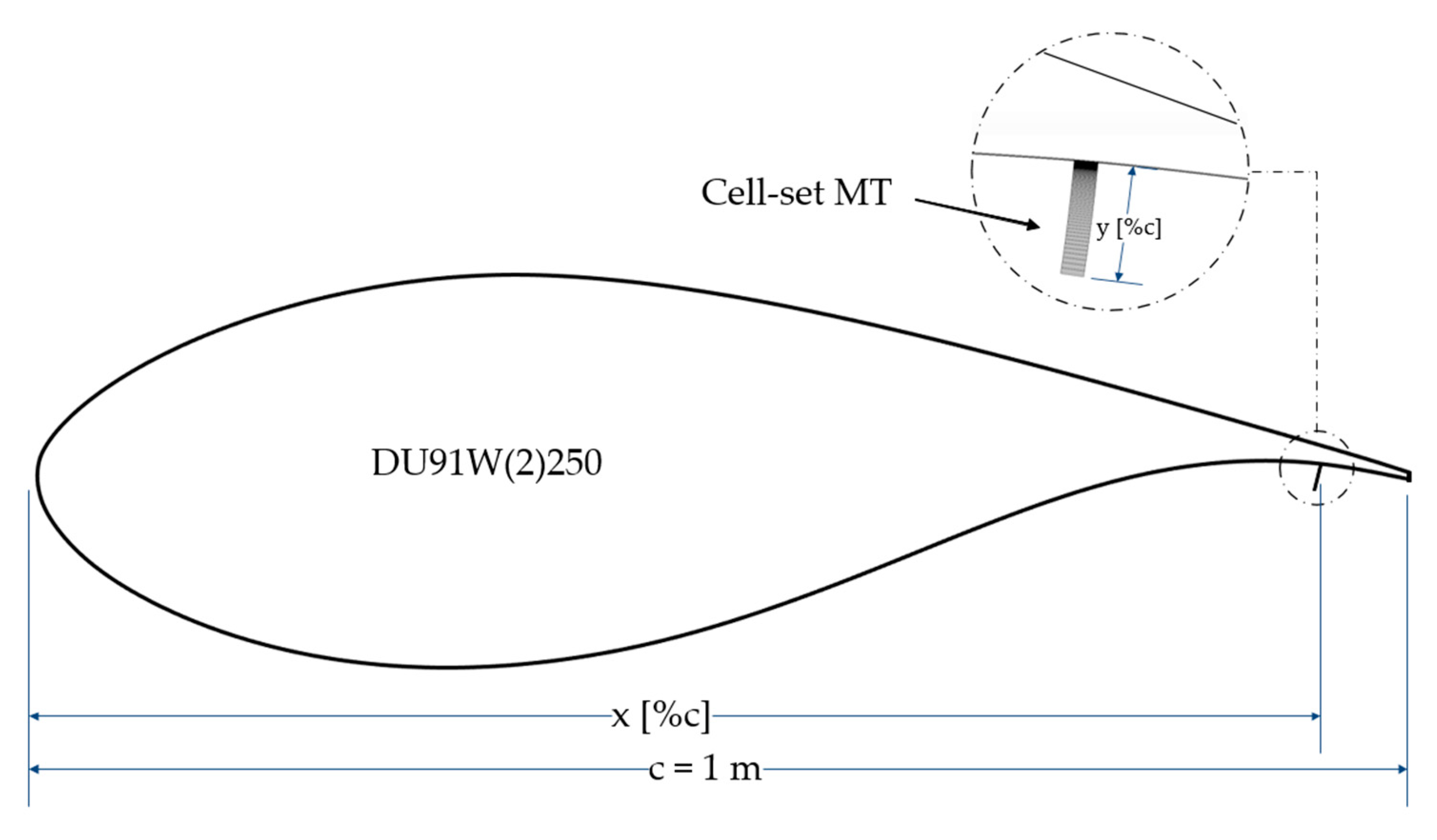
2.1. Numerical Setup

The present study has been based on a numerical analysis for MT implementation on a DU91W(2)250 airfoil. This airfoil is commonly used for horizontal axis wind turbine (HAWT) multi-megawatt applications; see the report of Jonkman et al. [30]. Two different models are presented in this manuscript: the cell-set model and the fully mesh model. In order perform numerical simulations, the STAR CCM+ v14.02.012 [31] commercial CFD software was selected.

The numerical scenarios were based on a DU91W(2)250 airfoil, where a two-dimensional O-mesh was generated around the aerodynamic profile. The radius of the mesh was set at R = $42\times c$, where c = 1 m is the airfoil chord length. This radius dimension was set in accordance with the recommendation from a study by Sørensen et al. [32]. As previously mentioned, two different models have been studied for the implementation of different MT configurations on the DU91W(2)250: the cell-set model was based on a clean airfoil grid domain without flow control devices, and all the scenarios for this model were based in that mesh. Conversely, the fully mesh cases needed different scenarios for each MT position and length. The structured grid where the cell-set model was applied was set at 207,740 finite elements. Similarly, for the fully mesh cases, the domain ascended to 232,415 cells, as the implementation of an MT close to the trailing edge area of the airfoil required a mesh refinement. A mesh dependency study on the DU91W(2)250 airfoil performed by Fernandez-Gamiz et al. [33] identified that the dependency of the mesh reached less than 4% for lift and drag coefficients calculations. Figure 1 illustrates an enlarged view of the clean mesh for the DU91W(2)250 aerodynamic profile. With the purpose of determining the first cell height, a normalization with the airfoil chord length was calculated, which was set at $\mathsf{\Delta }\mathrm{z}/\mathrm{c}=1.349\times {10}^{-6}$. The stretching in normal and chord-wise directions was achieved by tanh stretching functions which are based on Thompson et al. [34] and Vinokur [35]. The design of the grid was prepared to obtain dimensionless distances (y+ < 1) on the surface wall of the airfoil. The maximum skewness angle of the mesh reached 22.99°. The airfoil surface was set as a non-slip wall boundary type.

The simulations were carried out with a Reynolds number of $\mathrm{Re}=7\times {10}^6$, which is based on the airfoil chord length. Furthermore, the equations assigned to the fluid region of the computational domain were based on Reynolds-averaged Navier–Stokes (RANS) equations. Particularly, the shear stress transport (SST) model has been applied to the numerical simulations presented in this manuscript to model turbulence. As identified by Menter [36], the SST model accomplishes the fusion of the standard k-ε and k-ω turbulence model by means of a gradual variation on the turbulence properties: close to the surface wall, the calculations are determined relying on k-ω turbulence, while for the cells which are far from the wall boundary, k-ε standard turbulence is applied; see Kral [37]. The upwind algorithm was used for determining the pressure velocity coupling and a linear upwind second-order scheme was employed for the mesh discretization.

The physical properties of the air were established as follows: the air density was set at $\mathsf{\rho }=1.204\mathrm{kg}/{\mathrm{m}}^3$ and a dynamic viscosity value of $\mathsf{\mu }=1.829·{10}^{-5}$ Pa·s was introduced. The relative wind velocity value $V_{rel}=106.6\mathrm{m}/\mathrm{s}$.

The results have been represented by means of aerodynamic performance of the airfoil, also known as the lift-to-drag ratio, which represents the relationship between lift (C_L) and drag (C_D) dimensionless coefficients. Lift and drag coefficients were calculated through Equations (1) and (2), respectively.

$$C_L=\frac{L}{\frac{1}{2}\rho U_{\infty }{}^{2}c}$$

(1)

$$C_D=\frac{D}{\frac{1}{2}\rho U_{\infty }{}^{2}c}$$

(2)

2.2. MT Configurations

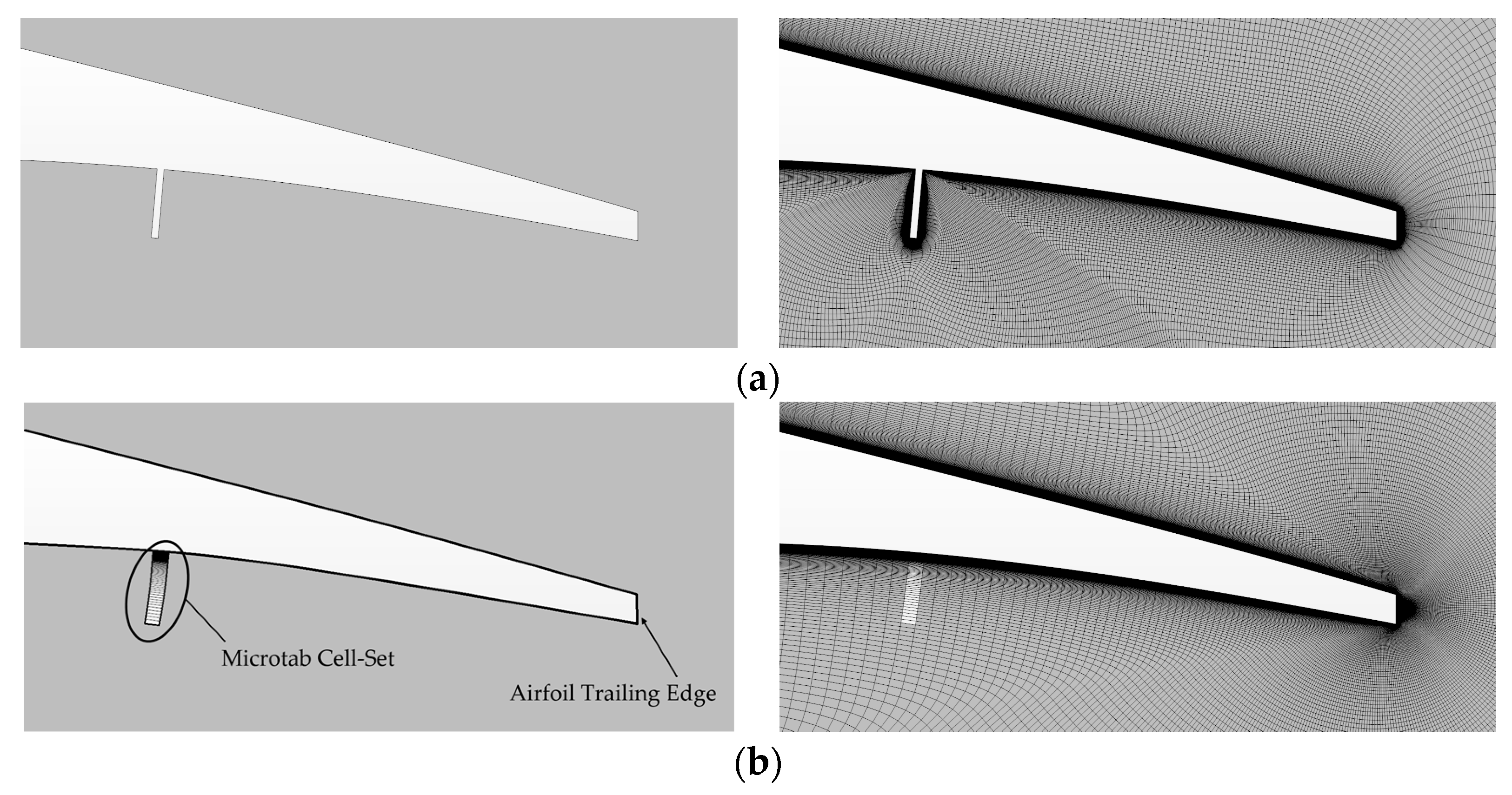
For the numerical simulations, different MT configurations were implemented. Figure 2 illustrates a sketch of the tab setup: x [%c] represents the MT position on the pressure side of the airfoil (relative position from the leading edge) and y [%c] is the MT length. In particular, the sketch shows a detailed view of an MT construction on a DU91W(2)250 airfoil based on the cell-set model.

MTs were located at two different positions near to the trailing edge of the airfoil: x [%c] = 93% and x [%c] = 95%. Three different MT lengths were established for the numerical analyses: y [%c] = 1.0%, y [%c] = 1.5% and y [%c] = 2.0%. The angles of attack (AoAs) ranged from 0 to 9°. Firstly, numerical simulations were performed with the fully mesh MTs and then the simulations were repeated by applying the cell-set model. All the cases have been named and classified in

Table 1. MT configuration cases.

Case	Short Ref.	x [%c]	y [%c]	Model
DU91W(2)250	clean	no MT	no MT	Fully mesh
DU91W(2)250_MTCS9310	CS9310	93	1.0	Cell-set
DU91W(2)250_MTCS9315	CS9315	93	1.5	Cell-set
DU91W(2)250_MTCS9320	CS9320	93	2.0	Cell-set
DU91W(2)250_MTCS9510	CS9510	95	1.0	Cell-set
DU91W(2)250_MTCS9515	CS9515	95	1.5	Cell-set
DU91W(2)250_MTCS9520	CS9520	95	2.0	Cell-set
DU91W(2)250_MTFM9310	FM9310	93	1.0	Fully mesh
DU91W(2)250_MTFM9315	FM9315	93	1.5	Fully mesh
DU91W(2)250_MTFM9320	FM9320	93	2.0	Fully mesh
DU91W(2)250_MTFM9510	FM9510	95	1.0	Fully mesh
DU91W(2)250_MTFM9515	FM9515	95	1.5	Fully mesh
DU91W(2)250_MTFM9520	FM9520	95	2.0	Fully mesh

.

2.3. Cell-Set Model

As previously reported, half of the simulations were based on the novel cell-set model. The verification of the cell-set model for MT implementation is the main point of the present study. This method was firstly used on a study by Ballesteros-Coll et al. [24] where a Gurney flap implementation was carried out. The model resulted to be considerably accurate to be implemented in other scenarios where small flow control devices have to be added on an airfoil. Nevertheless, when arbitrary modifications are required, the immersed boundary method (IBM) is a suitable option (see Reck [38]). For the generation of the cell-set model, firstly, the required geometry is generated onto the mesh, and subsequently, the cells which are around the mentioned geometry are selected by means of their IDs. Once a set of cells (cell set) is created, it is split from the fluid region by generating a new region. After that, a wall boundary limit is assigned to the region that has been built. Thus, this region follows the same equations that have been applied to the fluid region, RANS equations. Consequently, no re-meshing processes are needed in order to generate a new functional geometry. Figure 3 illustrates how small MTs are constructed by using the cell-set model compared to a fully mesh model.

3. Results

This section presents the results obtained with the cell-set model and the fully mesh model. Firstly, the performance of the model is visualized by means of representing different scenarios for MT implementation. Secondly, the errors of the cell-set model for each case have been determined with the aim of having quantitative results of the model. Additionally, qualitative results have been illustrated as a means to represent the cell-set model against the fully mesh model onto a scalar scene.

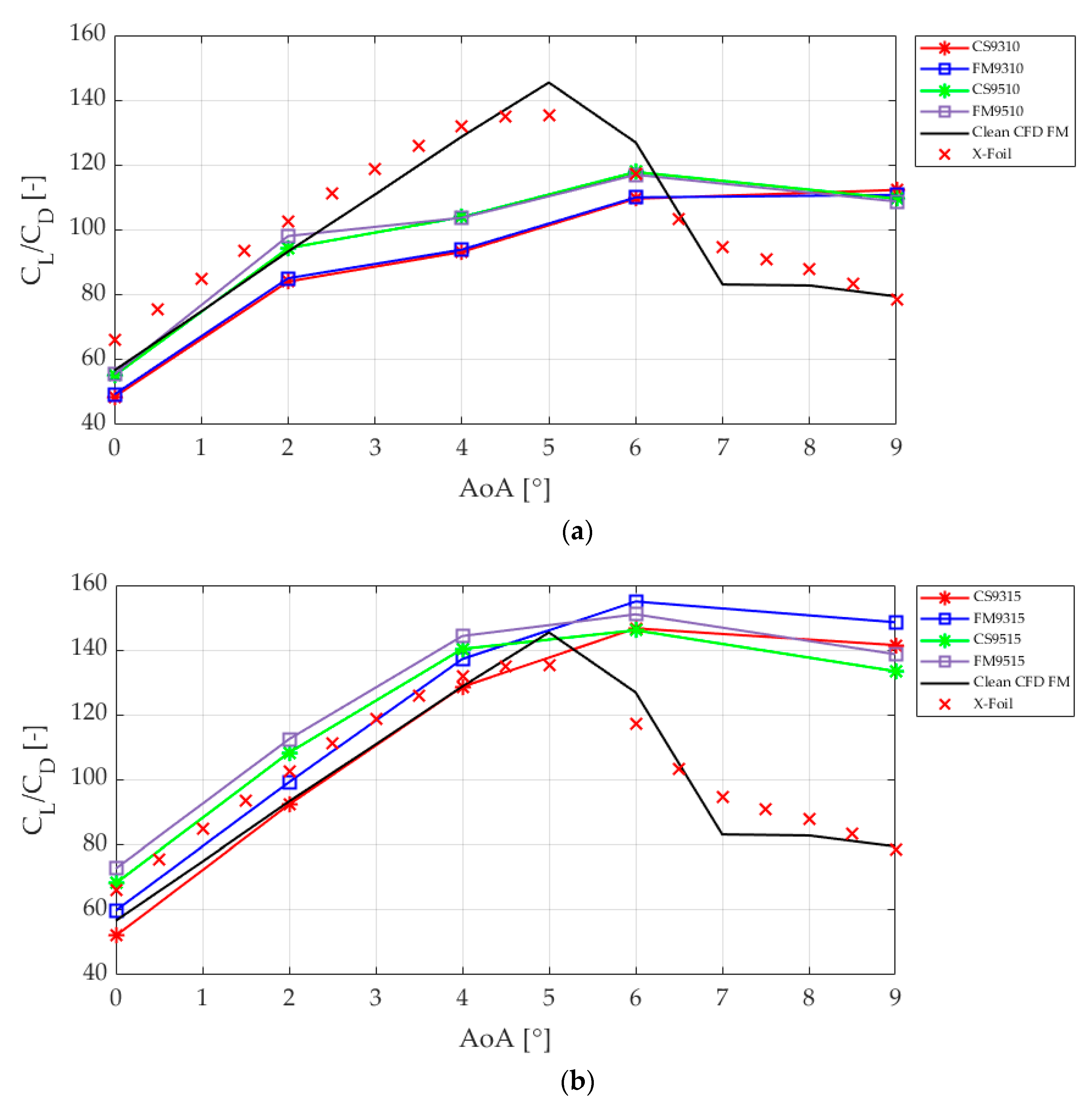
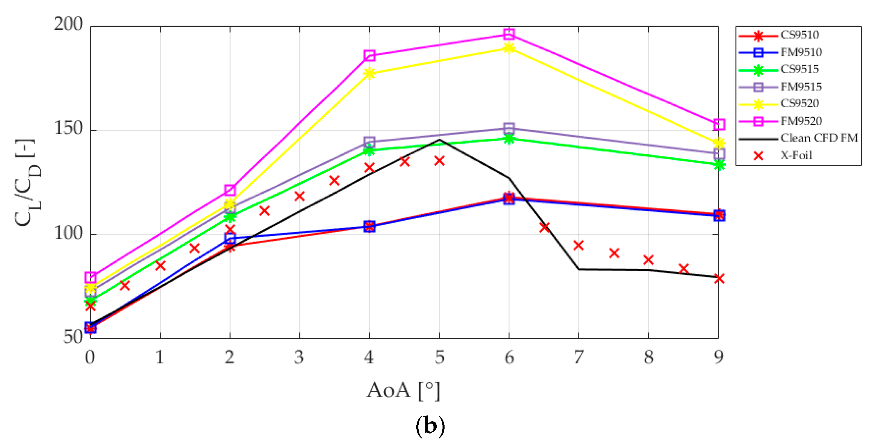
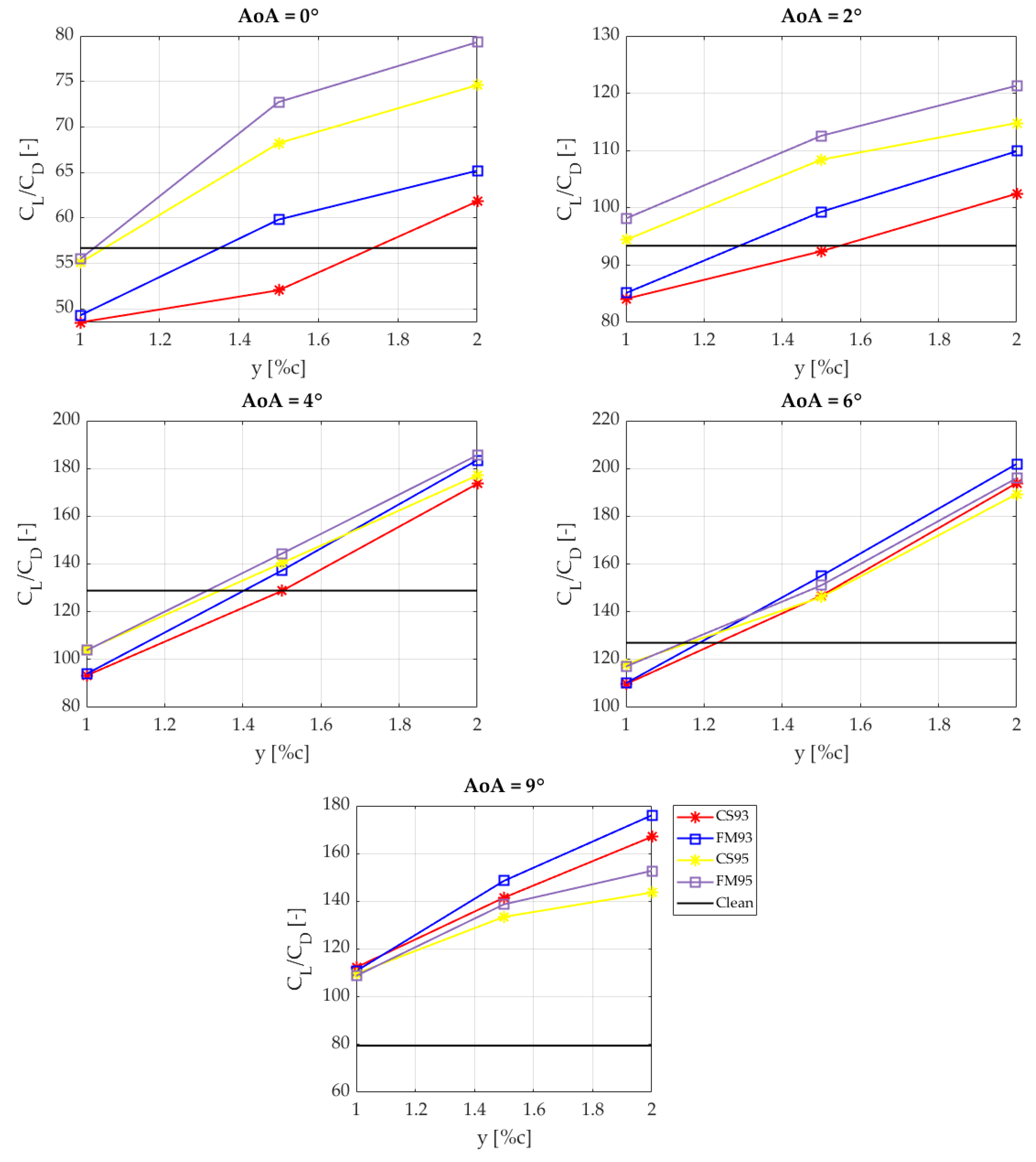
3.1. Cell-Set Model Performance for a Microtab Implementation

First of all, in order to study the effects of MT implementation for different positions on the pressure side of the airfoil (x [%c]), three plots have been generated; see Figure 4. Each plot illustrates the relationship between the aerodynamic performance of the airfoil (C_L/C_D, lift-to-drag ratio) and the AoA. There are six curves per plot: the continuous black line shows the values reached for the clean case, a DU91W(2)250 airfoil without flow control devices. These values are directly compared and validated against the ones obtained for a X-foil case (red-cross markers) from the DOWEC project which was carried out by Kooijman et al. [39] and Lindenburg [40]. Likewise, the values obtained from both models, cell-set and fully mesh, have been displayed in Figure 4. Red and green curves with asterisk markers show the performance values reached for the cell-set model while the blue and cyan curves with square markers present the performances for the fully mesh model. Two positions on the pressure side of the aerodynamic profile are introduced in each plot: x = 93% of c and x = 95% of c. In addition, for each device position, three different MT lengths are shown (one per plot) in Figure 4: y = 1.0% of c (a), y = 1.5% of c (b) and y = 2.0% of c (c).

As illustrated in Figure 4, the curve formed by the X-foil and the clean fully mesh curve follow a similar pattern. In the same way, the values obtained for the fully mesh model and the cell-set model show approximated ratios. Resulting data show that the position on the pressure side of the airfoil has an effect on the aerodynamic performance: for low AoAs, the performance values result to be higher for an MT located at 95% of c. By contrast, for AoAs higher than 6°, the airfoil with the MT located at 93% of c reaches higher C_L/C_D values. This effect is enhanced in the CS-FM9315, CS-FM9320, CS-FM9515 and CS-FM9520 cases, where y = 1.5% of c and y = 2.0% of c. For the CS-FM9310 and CS-FM9510 cases, the curves tend to be lower at x = 93% of c, for the whole AoA range, until a 9° AoA is reached. At that point, the profiles have similar aerodynamic performances.

The evidence suggests that the MT length variations on the pressure side of the airfoil affect more than the distance of the MT from the leading edge in terms of lift-to-drag ratio. Hence, in order to have a clearer description of the MT length variation effect on the aerodynamic performance of the airfoil, the illustrations of Figure 5 have been displayed. Each plot describes eight curves: the previous clean and X-foil curves are represented, with the purpose of following the same references. The remaining curves present the C_L/C_D ratios for the cell-set and fully mesh models. Magenta, cyan and blue curves with square markers show the fully mesh performances. On the contrary, yellow, green and red curves with asterisk markers describe the results for the cell-set model. There is one position of the MT per plot: x = 93% of c (a) and x = 95% of c (b).

Depending on the MT configuration, beneficial or detrimental properties could be added to the airfoil performance. In the previous illustrations of Figure 5, it is clearly presented that the variations in MT length play a significant role in terms of aerodynamic performance. At low values of AoA, MT implementation results to be beneficial in regard to performance, whereas longer MTs describe higher ratios. However, for low AoAs, the MT length variation effect on the C_L/C_D is not as noticeable as for high AoAs. At 2°, the curves start to diverge. For y = 1.5% of c and y = 2.0% of c, the performance values are enhanced with MT implementation, the curve of y = 2.0% of the chord length being the higher one of both of them. Nevertheless, after diverging at AoA = 2°, an MT with y = 1.0% of c length describes lower values than the clean profile. For this particular case, the profile starts to perform at increased ratios for AoAs higher than 6°.

After examining the curves, it can be concluded that CS-FM9320 is a suitable and optimum configuration among all the cases studied on this manuscript, closely followed by the CS-FM9520 configuration as the differences in x [%c] position imply minimal variations in the aerodynamic performance.

3.2. Error Calculations

With the aim of obtaining quantitative results for the cell-set model efficiency on an MT application, the relative error for each scenario was determined. Error calculations were performed by comparing the performance results obtained with the cell-set model to the ones obtained with fully mesh simulations. First of all, in order to visualize the errors generated by the cell-set model for each MT configuration, at different AoAs, all the scenes were analyzed case by case as it is illustrated in Figure 6. As previously presented in Section 3.1, aerodynamic performances have been represented for each MT configuration (x = 93% of c and x = 95% of c). The MT lengths have been designated from y = 1.0% of c to y = 2.0% of c. Each plot of Figure 6 displays five different curves: the black continuous line is the constant C_L/C_D ratio for a clean DU91W(2)250 airfoil without any flow control device implemented. Blue and cyan lines with square markers represent the values obtained for the fully mesh model for x = 93% of c and x = 95% of c, respectively. By contrast, red and yellow lines with asterisk markers show the calculations based on the cell-set model.

Figure 6 represents the error of the cell-set model by taking as a reference the fully mesh one. These relative errors have been calculated by operating with the following formulae: Equation (3) was used to determine the relative error per case. This formula compares the minimum $\left(\min \left(C_L/C_D\right)\right)$ and maximum $\left(\max \left(C_L/C_D\right)\right)$ lift-to-drag ratio values between both fully mesh and cell-set models and the result is presented as an error percentage. For some cases, the maximum value is reached with the cell-set model, and for other cases, with the fully mesh model. Moreover, the average relative error values per MT configuration were determined by Equation (4). Subsequently, the global relative error value was calculated by means of Equation (5). All the errors are represented in

Table 2. Relative error (%) per MT configuration case. Average errors are shown in the last row.

MT Case
AoA (°)	9310	9315	9320	9510	9515	9520
0	1.562	7.332	5.173	0.728	6.213	5.953
2	1.188	6.939	6.741	3.813	3.699	5.371
4	0.748	6.231	5.412	0.211	2.762	4.568
6	0.351	5.343	3.996	0.724	3.250	3.422
9	1.378	4.741	5.115	0.822	3.782	5.946
${\mathbf{e}}_{\mathit{a}\mathit{v}{\mathit{g}}_{\mathit{j}}} (\%)$	1.045	7.247	5.288	1.260	3.941	5.052

. The maximum relative error was reached at a 0° AoA with the CS9315 configuration with an ${\mathrm{e}}_{max}[\%]=$ 7.332% value. The global relative error value corresponds to ${\mathrm{e}}_g[\%]=$ 3.784%. In the study by Ballesteros-Coll et al. [24], the cell-set model reached a global relative error value of 1.13%. Therefore, it is considered that the cell-set model is accurate enough for its application in other scenarios, for the construction of small flow control devices.

$${\mathrm{e}}_{r_i}[\%]=\left(1-\frac{min\left(\frac{C_{L_i}}{C_{D_i}}\right)}{max\left(\frac{C_{L_i}}{C_{D_i}}\right)}\right)·100$$

(3)

$${\mathrm{e}}_{av{g}_j}[\%]=\frac{{\sum }_{i=1}^{N=5}{e}_{r_i}}{N}$$

(4)

$${\mathrm{e}}_g[\%]=\frac{{\sum }_{j=1}^{N=6}{e}_{av{g}_j}}{N}$$

(5)

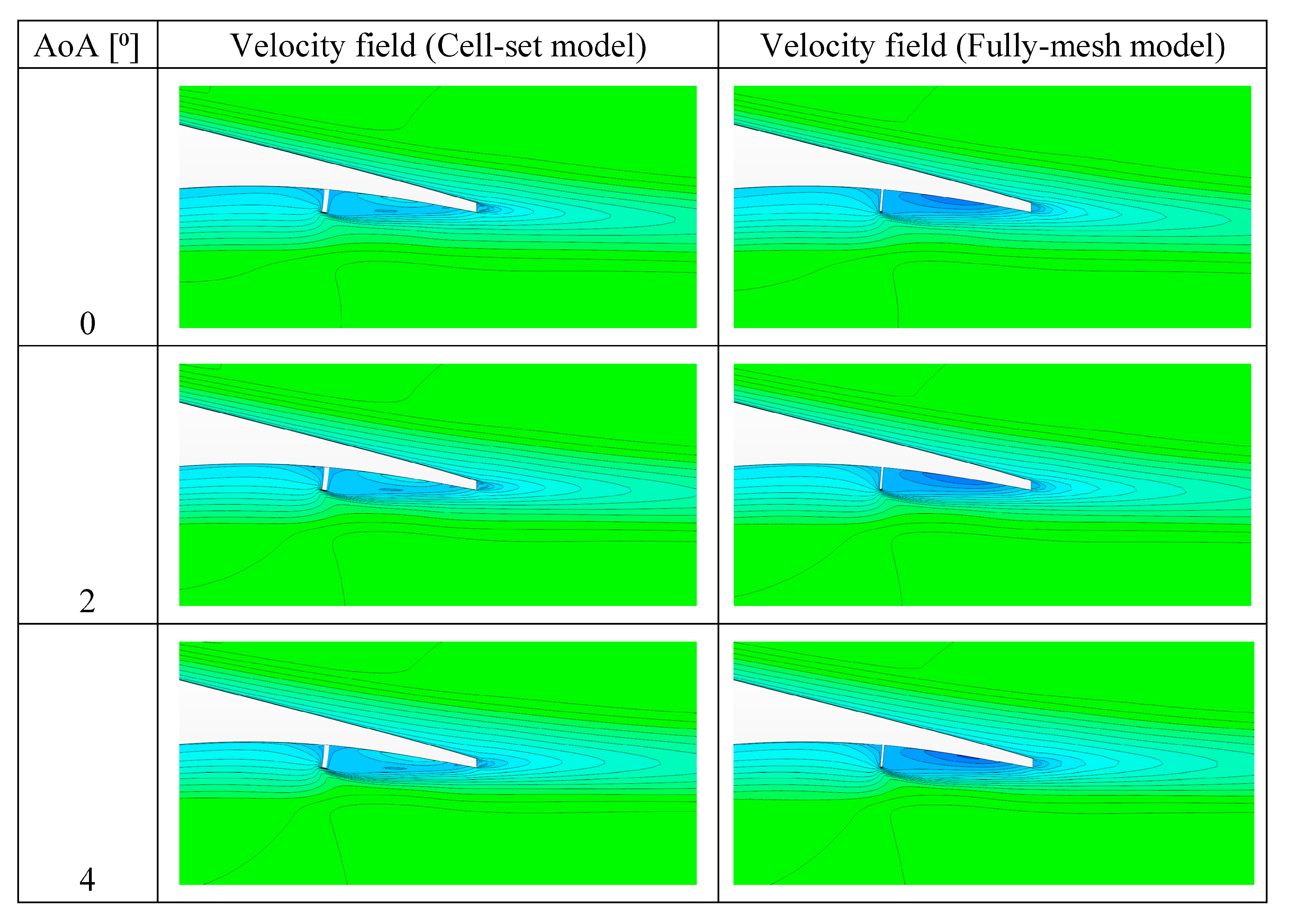
3.3. Qualitative Comparison between Cell-Set and Fully Mesh Models

In this section, a qualitative comparison between the fully mesh and the cell-set models is carried out. The images presented in Figure 7 show scalar scenes enlarged on the trailing edge area of the DU91W(2)250 airfoil with a CS9320 and a FM9320 MT implemented. Two snapshots have been presented for each AoA that has been studied: the cell-set model is on the left part and the fully mesh model is on the right part.

The correlation between illustrations is noticeable as the geometries created by the cell sets are significantly approximated to the fully mesh geometries. This factor contributes to a similar velocity field around the MT area and in the wake. Additionally, from 0 to 9°, different stream wakes generated by the change in the AoA are clearly represented in both models.

A comparison of pressure distribution was carried out by means of pressure coefficient (cp) values of the DU91W(2)250 airfoil surface. The CS-FM-9320 configuration (x = 93%; y = 2.0% of c) was selected as it resulted to be the one with the highest aerodynamic performance. Figure 8 represents the cp values for the mentioned case in the whole AoA range studied, for the fully mesh model and for the cell-set model. A continuous black line has been sketched in order to represent the airfoil dimensions. Positive gaps of cp are generated on the MT position and the aft loading is substantially enhanced on the MT area of the profile.

Different pressure levels show that the pressure drops between suction and pressure sides of the airfoil are enhanced for the fully mesh model in comparison with the cell-set model. This effect could be related to the more noticeable velocity field behind the MT in the fully-mesh (FM) cases; see right column of Figure 7.

The right side of Figure 8 illustrates an enhanced view of the pressure distribution in the MT region. Note that the mesh resolution is significantly smaller than the scale shown in the plot of Figure 8, making the error generated by mesh resolution almost unnoticeable. It can be barely noticed in the subplot where the pressure coefficient values for the cell-set model and fully mesh model are not aligned, as a consequence of the accuracy given by the cell-set.

4. Conclusions

In the current work, numerical simulations were carried out in order to study the cell-set model’s performance against a fully mesh model for MT implementation on a DU91W(2)250 airfoil. The cell-set model is an adaptable and versatile method to apply when the generation of new and small geometries into a computational domain is demanded. Additionally, no re-meshing processes are required in order to apply the model as the cells are split from the fluid region of the mesh, which is already generated. Consequently, the cell-set model saves mesh calculation times when a geometry has to be added or changed.

Firstly, it was determined that the numerical simulations based on the cell-set model and the fully mesh model formed similar patterns in terms of aerodynamic performance analysis. A global relative error value of ${\mathrm{e}}_g[\%]=$ 3.784% was reached and a maximum relative error value of ${\mathrm{e}}_{max}[\%]=$ 7.332% was calculated. Considering that the global relative error was significantly low, it can be concluded that the cell-set model is competent for the implementation of an MT in other scenarios. Furthermore, it has been also concluded that generally, when the construction of cells requires a high amount of structured elements, the error generated by the cell-set model tends to be increased.

Secondly, it was observed that the MT position changes along the pressure side of a DU91W(2)250 airfoil do not affect to the aerodynamic performance of the airfoil as much as the variation in the MT length. This factor contributed to a deeper analysis of the effects of MT length variations. Resulting data showed that the optimum MT configuration was reached with a CS-FM9320 configuration, where x = 93% of c (MT position from the airfoil leading edge) and y = 2.0% of c (MT length). The CS-FM9320 was closely followed by the CS-FM9520, as the MT position change did not have as much of an effect as the MT length.

Once quantitative evidence of the cell-set performance was obtained, a qualitative analysis was carried out wherein the effects produced on the velocity field by an MT implementation were displayed. Similar results were determined for both models: cell-set and fully mesh. These equally represented the effect of MT implementation since both showed similar wake shapes. In terms of pressure distribution, similar behavior has been observed in both models, with the fully mesh model being the one with the more noticeable pressure drop.

This cell-set based tool could be very helpful in order to perform successful parametric and optimization studies w here a high amount of simulations is required.

References

1. Howell, R.; Qin, N.; Edwards, J.; Durrani, N. Wind tunnel and numerical study of a small vertical axis wind turbine. Renew. Energy 2010, 35, 412–422. [Google Scholar] [CrossRef] [Green Version]
2. Vermeer, L.J.; Sørensen, J.N.; Crespo, A. Wind turbine wake aerodynamics. Prog. Aerosp. Sci. 2003, 39, 467–510. [Google Scholar] [CrossRef]
3. Aramendia Iradi, I.; Fernandez Gamiz, U.; Sancho Saiz, J.; Zulueta Guerrero, E. State of the art of active and passive flow control devices for wind turbines. DYNA Ing. E Ind. 2016, 91, 512–516. [Google Scholar] [CrossRef] [Green Version]
4. Aramendia, I.; Fernandez-Gamiz, U.; Ramos-Hernanz, J.A.; Sancho, J.; Lopez-Guede, J.M.; Zulueta, E. Flow control devices for wind turbines. In Energy Harvesting and Energy Efficiency; Bizon, N., Mahdavi Tabatabaei, N., Blaabjerg, F., Kurt, E., Eds.; Lecture Notes in Energy; Springer International Publishing: Cham, Switzerland, 2017; Volume 37, pp. 629–655. ISBN 978-3-319-49874-4. [Google Scholar]
5. Velte, C.M.; Hansen, M.O.L. Investigation of flow behind vortex generators by stereo particle image velocimetry on a thick airfoil near stall. Wind Energy 2013, 16, 775–785. [Google Scholar] [CrossRef]
6. Godard, G.; Stanislas, M. Control of a decelerating boundary layer. Part 1: Optimization of passive vortex generators. Aerosp. Sci. Technol. 2006, 10, 181–191. [Google Scholar] [CrossRef]
7. Gao, L.; Zhang, H.; Liu, Y.; Han, S. Effects of vortex generators on a blunt trailing-edge airfoil for wind turbines. Renew. Energy 2015, 76, 303–311. [Google Scholar] [CrossRef]
8. Timmer, W.A.; van Rooij, R. Summary of the Delft University wind turbine dedicated airfoils. J. Sol. Energy Eng. 2003, 125, 488–496. [Google Scholar] [CrossRef]
9. Timmer, W.A.; Schaffarczyk, A.P. The effect of roughness at high Reynolds numbers on the performance of aerofoil DU 97-W-300Mod. Wind Energy 2004, 7, 295–307. [Google Scholar] [CrossRef]
10. Martínez-Filgueira, P.; Fernandez-Gamiz, U.; Zulueta, E.; Errasti, I.; Fernandez-Gauna, B. Parametric study of low-profile vortex generators. Int. J. Hydrog. Energy 2017, 42, 17700–17712. [Google Scholar] [CrossRef]
11. Lin, J.C. Review of research on low-profile vortex generators to control boundary-layer separation. Prog. Aerosp. Sci. 2002, 38, 389–420. [Google Scholar] [CrossRef]
12. Kumar, P.M.; Samad, A. Introducing Gurney flap to Wells turbine blade and performance analysis with OpenFOAM. Ocean Eng. 2019, 187, 106212. [Google Scholar] [CrossRef]
13. Alber, J.; Pechlivanoglou, G.; Paschereit, C.O.; Twele, J.; Weinzierl, G. Parametric investigation of gurney flaps for the use on wind turbine blades. In Proceedings of the Volume 9: Oil and Gas Applications; Supercritical CO2 Power Cycles; Wind Energy; American Society of Mechanical Engineers, Charlotte, NC, USA, 26–30 June 2017; p. V009T49A015. [Google Scholar]
14. Aramendia, I.; Fernandez-Gamiz, U.; Zulueta, E.; Saenz-Aguirre, A.; Teso-Fz-Betoño, D. Parametric study of a gurney flap implementation in a DU91W(2)250 airfoil. Energies 2019, 12, 294. [Google Scholar] [CrossRef] [Green Version]
15. Zhu, B.; Huang, Y.; Zhang, Y. Energy harvesting properties of a flapping wing with an adaptive Gurney flap. Energy 2018, 152, 119–128. [Google Scholar] [CrossRef]
16. Saenz-Aguirre, A.; Fernandez-Gamiz, U.; Zulueta, E.; Ulazia, A.; Martinez-Rico, J. Optimal wind turbine operation by artificial neural network-based active gurney flap flow control. Sustainability 2019, 11, 2809. [Google Scholar] [CrossRef] [Green Version]
17. Gruschwitz, E.; Schrenk, O. A Simple Method for Increasing the Lift of Airplane Wings by Means of Flaps; NASA: Washington, DC, USA, 1933. [Google Scholar]
18. Van Dam, C.P.; Nakafuji, D.Y.; Bauer, C.; Standish, K.; Chao, D. Computational design and analysis of a microtab-based aerodynamic load control system for lifting surfaces. In Proceedings of the MEMS Components and Applications for Industry, Automobiles, Aerospace, and Communication II, San Jose, CA, USA, 25–31 January 2003; Volume 4981. [Google Scholar]
19. Baker, J.P.; Standish, K.J.; van Dam, C.P. Two-dimensional wind tunnel and computational investigation of a microtab modified airfoil. J. Aircr. 2007, 44, 563–572. [Google Scholar] [CrossRef]
20. Ebrahimi, A.; Movahhedi, M. Wind turbine power improvement utilizing passive flow control with microtab. Energy 2018, 150, 575–582. [Google Scholar] [CrossRef]
21. Cooperman, A.M.; Chow, R.; van Dam, C.P. Active load control of a wind turbine airfoil using microtabs. J. Aircr. 2013, 50, 1150–1158. [Google Scholar] [CrossRef]
22. Johnson, S.J.; Baker, J.P.; van Dam, C.P.; Berg, D. An overview of active load control techniques for wind turbines with an emphasis on microtabs. Wind Energy 2010, 13, 239–253. [Google Scholar] [CrossRef]
23. Sanderse, B.; Pijl, S.P.; Koren, B. Review of computational fluid dynamics for wind turbine wake aerodynamics: Review of CFD for wind turbine wake aerodynamics. Wind Energy 2011, 14, 799–819. [Google Scholar] [CrossRef] [Green Version]
24. Ballesteros-Coll, A.; Fernandez-Gamiz, U.; Aramendia, I.; Zulueta, E.; Lopez-Guede, J.M. Computational methods for modelling and optimization of flow control devices. Energies 2020, 13, 3710. [Google Scholar] [CrossRef]
25. Jirasek, A. Vortex-generator model and its application to flow control. J. Aircr. 2005, 42, 1486–1491. [Google Scholar] [CrossRef]
26. Errasti, I.; Fernández-Gamiz, U.; Martínez-Filgueira, P.; Blanco, J. Source term modelling of vane-type vortex generators under adverse pressure gradient in OpenFOAM. Energies 2019, 12, 605. [Google Scholar] [CrossRef] [Green Version]
27. Chillon, S.; Uriarte-Uriarte, A.; Aramendia, I.; Martínez-Filgueira, P.; Fernandez-Gamiz, U.; Ibarra-Udaeta, I. jBAY modeling of vane-type vortex generators and study on airfoil aerodynamic performance. Energies 2020, 13, 2423. [Google Scholar] [CrossRef]
28. Fernandez, U.; Réthoré, P.-E.; Sørensen, N.N.; Velte, C.M.; Zahle, F.; Egusquiza, E. Comparison of four different models of vortex generators. In Proceedings of the EWEA 2012—European Wind Energy Conference & Exhibition; European Wind Energy Association (EWEA), Copenhagen, Denmark, 16–19 April 2012. [Google Scholar]
29. Fernandez-Gamiz, U.; Gomez-Mármol, M.; Chacón-Rebollo, T. Computational modeling of gurney flaps and microtabs by POD method. Energies 2018, 11, 2091. [Google Scholar] [CrossRef] [Green Version]
30. Jonkman, J.; Butterfield, S.; Musial, W.; Scott, G. Definition of a 5-MW Reference Wind Turbine for Offshore System Development; Technical Report No. NREL/TP-500-38060; National Renewable Energy Lab.: Golden, CO, USA, 2009; p. 7. [Google Scholar]
31. Siemens Star CCM+ Version 14.02.012. Available online: https://www.plm.automation.siemens.com/global/en/ (accessed on 3 February 2020).
32. Sørensen, N.N.; Mendez, B.; Munoz, A.; Sieros, G.; Jost, E.; Lutz, T.; Papadakis, G.; Voutsinas, S.; Barakos, G.N.; Colonia, S.; et al. CFD code comparison for 2D airfoil flows. J. Phys. Conf. Ser. 2016, 753, 082019. [Google Scholar] [CrossRef] [Green Version]
33. Fernandez-Gamiz, U.; Zulueta, E.; Boyano, A.; Ramos-Hernanz, J.; Lopez-Guede, J. Microtab design and implementation on a 5 MW wind turbine. Appl. Sci. 2017, 7, 536. [Google Scholar] [CrossRef]
34. Thompson, J.F.; Warsi, Z.U.A.; Mastin, C.W. Numerical Grid Generation: Foundations and Applications; Elsevier Science (North-Holland Publishing Co.): New York, NY, USA, 1985; ISBN 978-0-444-00985-2. [Google Scholar]
35. Vinokur, M. On one-dimensional stretching functions for finite-difference calculations. J. Comput. Phys. 1983, 50, 215–234. [Google Scholar] [CrossRef] [Green Version]
36. Menter, F.R. Two-equation eddy-viscosity turbulence models for engineering applications. AIAA J. 1994, 32, 1598–1605. [Google Scholar] [CrossRef] [Green Version]
37. Kral, L.D. Recent experience with different turbulence models applied to the calculation of flow over aircraft components. Prog. Aerosp. Sci. 1998, 34, 481–541. [Google Scholar] [CrossRef]
38. Reck, M. Computational Fluid Dynamics, with Detached Eddy Simulation and the Immersed Boundary Technique, Applied to Oscillating Airfoils and Vortex Generators. Ph.D. Thesis, Technical University of Denmark, Lyngby, Denmark, 28 September 2005. [Google Scholar]
39. Kooijman, H.J.T.; Lindenburg, C.; Winkelaar, D.; Hooft, E.L.V.D. Aero-Elastic Modelling of the DOWEC 6 MWpre-Design in PHATAS; DOWEC-F1W2-HJK-01-046/9; Tech. Rep. ECN-CX-01-135, DOWEC 10046_009; Energy Research Center of the Netherlands: Petten, The Netherlands, 2003. [Google Scholar]
40. Lindenburg, C. Aeroelastic Modelling of the LMH64-5 Blade; DOWEC-02-KL-083/0, DOWEC 10083_001; Energy Research Center of the Netherlands: Petten, The Netherlands, 2002. [Google Scholar]
Figure 1. DU91W(2)250 mesh, centered view. The snapshot shows a clean profile without any flow control device implemented.
Energies 13 06723 g001
Figure 2. Sketch of the microtab (MT) setup. The relative position and length of the MT are determined by x [%c] and y [%c], respectively. The detail view shows an MT cell-set construction for an x [%c] = 93% and y [%c] = 1.0% configuration.
Energies 13 06723 g002
Figure 3. Comparison of the models for the generation of new geometries (microtabs): (a) fully-mesh model, DU91W(2)250_MTFM9310; (b) cell-set model, DU91W(2)250_MTCS9310. Snapshots show the mesh distribution around trailing edge area of the airfoil.
Energies 13 06723 g003
Figure 4. Aerodynamic performance curves (CL/CD, lift-to-drag ratio) for different positions on the pressure side of a DU91W(2)250 airfoil: x = 93% of c and x = 95% of c. Each plot has one MT length (y) assigned: (a) y = 1.0% of c; (b) y = 1.5% of c; (c) y = 2.0% of c. Angles of attack (AoAs) range between 0 and 9°.
Energies 13 06723 g004aEnergies 13 06723 g004b
Figure 5. Aerodynamic performance curves (CL/CD, lift-to-drag ratio) for different MT lengths implemented on a DU91W(2)250 airfoil: (a) location of the MT at x = 93% of c and (b) location of the MT at x = 95% of c. AoAs range between 0 and 9°.
Energies 13 06723 g005aEnergies 13 06723 g005b
Figure 6. MT configuration cases. Each plot shows the effects of MT length variation on the CL/CD lift-to-drag ratio. A single AoA per plot is represented. AoAs range between 0 and 9°.
Energies 13 06723 g006
Figure 7. Qualitative comparison of velocity scalar field of the cell-set model and fully mesh model for MT implementation on a DU91W(2)250 airfoil. MT9320 configuration: x [%c] = 93%; y [%c] = 2.0%.
Energies 13 06723 g007aEnergies 13 06723 g007b
Figure 8. Pressure distribution of the DU91W(2)250_MTCS9320 and DU91W(2)250_MTFM9320 cases represented with the pressure coefficient (cp) at AoA = 0°, 2°, 4°, 6° and 9°. The subplot shows an enlarged view of the MT area.
Energies 13 06723 g008