Predictive Control of District Heating System Using Multi-Stage Nonlinear Approximation with Selective Memory

Abstract

Innovative heating networks with a hybrid generation park can make an important contribution to the energy turnaround. By integrating heat from several heat generators and a high proportion of different renewable energies, they also have a high degree of flexibility. Optimizing the operation of such systems is a complex task due to the diversity of producers, the use of storage systems with stratified charging and continuous changes in system properties. Besides, it is necessary to consider conflicting economic and ecological targets. Operational optimization of district heating systems using nonlinear models is underrepresented in practice and science. Considering ecological and economic targets, the current work focuses on developing a procedure for an operational optimization, which ensures a continuous optimal operation of the heat and power generators of a local heating network. The approach presented uses machine learning methods, including Gaussian process regressions for a repeatedly updated multi-stage approximation of the nonlinear system behavior. For the formation of the approximation models, a selection algorithm is utilized to choose only essential and current process data. By using a global optimization algorithm, a multi-objective optimal setting of the controllable variables of the system can be found in feasible time. Implemented in the control system of a dynamic simulation, significant improvements of the target variables (operating costs, CO₂ emissions) can be seen in comparison with a standard control system. The investigation of different scenarios illustrates the high relevance of the presented methodology.

1. Introduction

The German government-driven turnaround towards the increased use of renewable energy sources has far-reaching effects on the structure of the national energy supply [1]. In addition to effects on the electricity sector, this naturally also affects the heating market to achieve the energy policy objectives at the global, European and national level. To this end, it is necessary to further develop heat supply concepts and adapt them to the requirements of a holistic energy turnaround. Systems of the future, both centralized and decentralized, will be characterized by a high proportion of renewable energy with low primary energy use and low CO₂ emissions, as well as a high degree of flexibility due to the fluctuation of renewable energies. Energy industry conditions that change over time, e.g., on the electricity exchange, are also experiencing increasing relevance [2].

In a district in Germany with around 100 residential units the opportunity is offered to develop an innovative method for optimizing the use of heat and power generation. The heat supply of the hybrid district heating network consists of a solar thermal plant, an electrically driven heat pump, a natural gas-powered cogeneration unit (also called combined heat and power, abbreviated with CHP), a natural gas boiler and a heat storage with internally stratified charge lances. As shown by Pater [2], the use of such a hybrid installation can be very beneficial for increasing the renewable energy share, even though the operation is very complex and more advanced algorithms are required to fully exploit the potential. The challenges in operating such a system are the need to continuously consider changing boundary conditions and system properties and to decide in a practical time for optimal use of the controllable heat suppliers regarding divergent operational targets (e.g., operating costs, CO₂ emissions). Model-based approaches, which learn from historical data and map the prospective nonlinear system behavior, are a promising solution. However, multi-objective optimization, which involves predicting the complex future trends, places very high demands on the prediction quality of these models and their computational effort. A difficult tension exists between accuracy and speed, leading to the research questions of which target shall be addressed in this work:

• How can a multivariate prognosis of the nonlinear system behavior be created, enabling the target variables to be optimized as well as approximated with sufficient accuracy and in a sufficiently short time?
• What is the advantage of an operational optimization concept compared to a standard control?

The structure of this work is as follows: After a literature review on the topic of operational optimization of local heating networks and the presentation of the research gap in Section 2, Section 3 describes the dynamic simulation of the local heating supply under construction. Section 4 presents the approach to model predictive control (MPC) through a multi-stage approximation, which is implemented in the dynamic simulation and sets an optimal operation in a time-discrete manner. Since the optimization depends to a large extent on the regulatory framework, Section 5 considers three different scenarios that are relevant in Germany and differ, for example, in the design of state incentives. A discussion of the results of the optimization in the simulation environment is provided in Section 6 for the considered scenarios as well as for different optimization goals. Section 7 finally concludes this work with a summary and an outlook on future work, also taking into account the grid stabilization and sector coupling.

2. Literature Review

Standard controls, as used in practice for hybrid local heating systems with storage solutions, prioritize the heat generators depending on their economic efficiency and have one or more control variables, for example, the storage tanks charge state or the temperature in the local heating network. This ensures that the heat demand is covered in line with the costs. However, future changes are not considered.

For many years, however, methods have been developed with which future influences and developments can be considered for the planning of operation. These are based on a system modelling via energy balances, which are solved using the formulation of (mixed-)integer linear programs (MILP). The result is the optimal switch-on sequence of the available devices concerning a target value such as the operating costs at discrete time intervals, considering boundaries such as the minimum switch-on time of individual devices. A great advantage of linearization is the guarantee of finding a global optimum or a statement about the proximity to it. Verrilli et al. [3] developed a method for online operational optimization of a local heating supply with a fluctuating load to reduce the operating and maintenance costs considering the predicted heat load. The system was modeled using energy balances and optimized using mixed-integer programs. Stange et al. [4] also describe such an operational optimization, which has been developed over several decades. Guzek et al. [5] also use linearized models for optimization with integer programming, whereby the linearization is partly data-based, i.e., partly based on historical measurement data from the plant. However, the procedure is not used for online optimization, i.e., continuous tracking of the optimization based on current information.

The literature also shows that the consideration of heat storages poses problems. To take into account a certain stratification in heat storages, in Steen et al. [6] such storage is divided into two separate layers with separate energy contents to be able to optimize the problem via MILP. Lengyl et al. [7] divide the storage tank into different layers with constant temperature for different heat suppliers. It is not clear whether such a procedure allows online operational optimization. A good overview of further work on the optimization of energy supply systems is provided in Talebi et al. [8], whereby it becomes clear that linearization of the problem and the use of MILP is state of the art. The biggest challenge in the formulation of linear programs for optimal operational planning is the necessary linearization of the problem. Also, endogenous variables, i.e., those that depend on themselves, cannot be dealt with in the determination of target variables, as summarized by Urbanucci [9]. This circumstance is especially disadvantageous when considering thermal storage systems with stratified charging systems, where the operating behavior is influenced by the temperature stratification.

To circumvent the mentioned limitations, nonlinear model-based predictive controls from the field of machine learning can be used. For these, databased models are created with which it is possible to map nonlinear relationships. The use of nonlinear models from the field of machine learning has been used for a long time for the prediction of, e.g., weather data. Two examples among many are presented in Kato et al. [10] and Xie [11] with the prediction of the heat demand of buildings through artificial neural networks (ANN). However, there are also examples of online operational optimization. Kaiser et al. [12] apply their developed SINDY algorithm to various examples of dynamic systems in a simulation environment, which automatically identifies the respective system behavior based on measurement data and shows good prediction properties also for nonlinear system behavior. Limon and Maciejowski [13] also present an approach for data-based modeling and operational optimization, for the example of a torque-operated pendulum with good results. The authors fear, however, that higher-dimensional problems will reach their limits concerning computing time. There are only a few examples in the field of operational optimization of local heat supply systems. Cox et al. [14] use ANNs to optimize the operation of a refrigeration network, but only to represent the behavior of the cold storage as a thermal mass. Nevertheless, the results show that operational optimization is possible and can lead to advantageous operation modes.

The literature review shows that there is a research gap regarding the use of databased nonlinear models for online operational optimization of local heating systems. The use of these models can lead to greater proximity to reality due to the actual occurrence of nonlinearities and the intrinsic actuality of the models. In addition, multi-objective optimizations in a short time and further analysis, such as optimization under consideration of uncertainties, are possible. Such databased, nonlinear modeling for online operational optimization of a local heating supply is, therefore, to be presented in this work to contribute to its meaningful operation in the conflict between economic and ecological requirements. In the future, the approach presented here will be applied to a newly build local heating supply in Germany, which will be discussed in the next section.

3. Description of Simulation Model

The simulation model is the image of a heat plant in Kempen on the Lower Rhine, Germany, which has been in operation since the end of 2019. Connected to a fourth-generation heating network [15], it will supply around 900 MWh of heat per year to a total of 100 residential units. The supply or return temperature of the heating network is 55 or 35 °C throughout the year.

Due to the low supply temperature of 55 °C, the heating network enables the efficient use of heat generators based on renewable energies. In addition to a natural gas cogeneration module with 50 kW_el/90 kW_th, an electric geothermal heat pump with 60 kW_th and a solar thermal plant consisting of 211 m² of compound parabolic concentrator vacuum tube collectors feed heat into a 50 m³ heat storage with a stratified charging system. For thermal security of supply and for peak load, a natural gas boiler can supply up to 725 kW_th of heat directly to the heating network, see Figure 1.

The heat station was mapped in detail in the simulation environment Matlab^®/Simulink^® with the freely accessible toolbox CARNOT [16]. The toolbox contains models for the thermodynamic calculation of components of the heating, ventilation and air conditioning (HVAC) category.

Each device model was parameterized according to the manufacturer’s specifications or test protocols of certified test institutes regarding thermal and electrical power curves as well as control and regulation. The characteristic values of the high-resolution 3D model [17] of the earth probe field are derived from the results of a thermal response test of the subsurface. In the simulation, the storage is vertically subdivided into a total of 50 calculation nodes, while maintaining a Courant-Friedrichs-Lewy number [18] less than one and in order to represent a realistic temperature stratification in the storage tank.

The heating network topology is irrelevant for the simulation of the heating station, only the sum of the heat loads occurring in the network is relevant. The total load consists of the heat demand for space heating and hot water preparation of the connected residential units plus distribution losses in the network. For an approximate calculation of the total building heating load [19], a secondary energy consumption of a new building in Germany of about 40 kWh/(m²-a) at 1400 h of full use and a total living space of an estimated 14,000 m² was assumed. With a design outside temperature of −8.1 °C at the grid site and a heating limit temperature of 12 °C, a linear model was used to calculate an hourly resolved heating load curve for a complete year. The freely available tool DHWcalc [20] was used to calculate the heat demand for domestic hot water preparation. This tool generates tap profiles for domestic hot water on a statistical basis. By means of an assumed temperature spread between cold and hot water of 30 K and the tapping profile the domestic hot water heat demand was determined. An approximate heat loss calculation for the heating network considering the structural and technical conditions as well as the thermal boundary conditions [21] completes the calculation of the temporally resolved total heat load. In the last step, the model of the heating network received a thermal mass in the order of magnitude of the real model. Another important boundary condition is the weather (global radiation, outside air temperature, wind speed, degree of coverage, etc.). For this purpose, data from a weather station operated by the German Weather Service in nearby Krefeld is used. To calculate the economic target (operating costs), energy price data (stock market price of natural gas [22] and electricity [23])) as well as taxes, levies and government subsidies in Germany must also be taken into account. The ecological target (CO₂ emissions), on the other hand, is determined according to norm [24].

The classical control strategy of energy supply systems is based on a simple switch-on sequence of the heat generators. Thereby the units switch on in descending order of their efficiency (for further information see Section 5). Since primarily the weather conditions determine the heat output of the solar thermal system, it cannot be switched on arbitrarily. This results in the following switch-on sequence: solar thermal (ST), combined heat and power plant (CHP), heat pump (HP), natural gas boiler (NGB). The latter only feeds directly into the heating network and supplies the residual power to maintain the required network flow temperature. The remaining heat generators feed only into the heat storage, which means that their heat generation is decoupled from the heat demand of the network over time. The solar thermal system always supplies heat as soon as the irradiation is sufficient to reach the required target value. The CHP starts as soon as the center of the storage falls below a temperature limit. The heat pump switches in addition, if in the upper third of the storage a temperature limit value is fallen below. The boiler starts up when supply temperature is below a set point. This is illustrated in Figure 2.

Table 1. Results of a simulation for the operation of the local heating network under standard control.

Unit	Qth,out in MWh	Ael,in in MWh	Ael,out in MWh	Share in %
ST	125.9	0.2	-	14.6
CHP	440.0	-	226.7	51.2
HP	148.6	33.9	-	17.3
NGB	145.0	-	-	16.9

shows the results of an exemplary simulation over the period of one year, the heat generation (Q_th,out) as well as the electrical power consumption and generation of the individual devices (A_el,in or A_el,out) as a consequence of the described regulation. The not shown heat losses in the distribution network account for about 10% of the total heat demand. The heat losses were estimated by applying heat transport equations [21] using the real installation situation and soil temperature curve.

4. Model Predictive Control Approach

The operational management of the heat supply for a hybrid local heating network can be sensibly evaluated with ecological as well as economic targets in two directions, e.g., ecologically with the CO₂ emissions and economically with the operating costs. Often there is a conflict of objectives because ecological and economical operation are not compatible with each other.

The aim of this work is therefore to develop a multi-objective operational optimization of the heat supply for a hybrid local heating network, considering as much information as possible about current and future conditions and the general system behavior. To achieve this goal, a mathematical description of the system is first required, with which the future behavior or the target variables to be investigated are described sufficiently precisely in dependence of various influencing variables. This system description is then the starting point for an optimization algorithm to determine the optimal settings of the controllable variables as quickly as possible within a time horizon to be defined. A standard control according to Section 3 serves as reference and benchmark for the performed investigations.

Against the direct use of the dynamic simulation for the operational optimization speaks the high time requirement of approx. two minutes per simulated day, which makes an evaluation of thousands of different settings of the controllable variables for the optimization in practical time (in less than one minute) impossible. But also, the possibility of convergence problems and other errors that could lead to a termination prohibit the use of simulation. In addition, the dynamic simulation model would have to be regularly adapted to the current real conditions (e.g., a deterioration of the system due to fouling in the heat exchangers), which is a great effort.

An alternative is the use of approximation models, which represent the underlying dynamic system behavior discretely in time and automatically consider changes in the system behavior. This section describes how a nonlinear approximation for model-predictive control is developed with the help of the simulation described in Section 3.

4.1. Approximation of Economical and Ecological Objectives

The model-based operational optimization developed here uses an approximation of the nonlinear system responses. Considering the target variables CO₂ emissions and operating costs, the goal is to minimize the system response $y$ over a defined prediction horizon $t_p$. The mathematical formulation of the optimization problem of the system response over the prediction horizon $y_{tp}$ shows Equation (1):

$$\begin{array}{c}{y}_{tp}={\displaystyle {\displaystyle \sum }_{t=0}^{t=t_p}}{y}_t\left(X,Z,u\right)·w_t\\ \underset{w.r.tX|\left(u,Z\right)}{\min }{y}_{tp}\end{array}$$

(1)

Here, $X$ represents the controllable variables (thermal power of CHP and HP) and $Z$ the system variables (i.a. heat load, global radiation, ambient temperature) over the course of the prediction horizon $t_p$ and $u$ the state variables (storage temperatures). The weighting vector $w_t$ serves to compensate for increasing uncertainties in the prediction horizon. The system responses $y_{tp}$ are the CO₂ emissions $E$ as well as the operating costs $K$, which result from the use of secondary energy for heat supply in a fixed time interval, here one hour, and are summed up over the considered time horizon.

Equation (2) makes it clear that the emissions are a function of the gas input in CHP $Q_{g,CHP}$ and boiler $Q_{g,NGB}$ as well as the electricity production of CHP module $Q_{el,CHP}$ (credit for electricity production substituted elsewhere) and the electricity consumption of the heat pump $Q_{el,HP}$. Equation (3) shows that the costs are additionally a function of the electricity price $c_{el}$, the gas price $c_g$ and the emission costs $c_e$ (summarized as $C$):

$$E=f\left(Q_{g,CHP},Q_{g,NGB},Q_{el,CHP},Q_{el,HP}\right)$$

(2)

$$K=f\left(Q_{g,CHP},Q_{g,NGB},Q_{el,CHP},Q_{el,HP},C\right)$$

(3)

The functional relationships for costs, prices and emissions are defined and known via standards, laws and regulations and other sources. The secondary energy input in the heat/electricity generators $Q_{g/el}$ can be considered as a function of the generation powers (see Equation (4)):

$$Q_{g/el}=f\left({\dot{Q}}_{CHP/NGB/HP}\right)$$

(4)

As described in Section 3, the heat load ${\dot{Q}}_L$ is covered by a thermal storage and a peak load boiler (${\dot{Q}}_{NGB})$. The latter provides heat when the thermal power of the storage tank ${\dot{Q}}_{TS}$ is not sufficient (see Equation (5)):

$${\dot{Q}}_{NGB}=\max \left(0,{\dot{Q}}_L-{\dot{Q}}_{TS}\right)$$

(5)

How much thermal output the storage and the boiler provide in a time interval depends on the temperature distribution of the storage tank ${\overrightarrow{T}}_{TS}$ and the heat load ${\dot{Q}}_L$ in the respective time interval. If the uppermost storage layer is above the required network temperature (55 °C), the output can be covered proportionally. If the temperature falls below this value, the storage power is also dependent on the average thermal power of the CHP module ${\dot{Q}}_{CHP}$ and heat pump ${\dot{Q}}_{HP}$, the power of the solar thermal plant ${\dot{Q}}_{ST}$ and, due to the heat losses of the storage tank, the ambient air temperature $T_{amb}$, see Equation (6):

$${\dot{Q}}_{TS}=f\left({\overrightarrow{T}}_{TS},{\dot{Q}}_{CHP},{\dot{Q}}_{HP},{\dot{Q}}_{ST},T_{amb},{\dot{Q}}_L\right)$$

(6)

The average thermal power of the CHP module and HP are the controllable variables $X$ and are therefore known or can be, to some extent, freely selected for optimization. The average thermal output of the solar thermal system is not known, but can be considered in a first approximation as a function of the global radiation $\dot{G}$ as well as the ambient temperature and the storage temperatures:

$${\dot{Q}}_{ST}=f\left(\dot{G},{\overrightarrow{T}}_{TS},T_{amb}\right)$$

(7)

Since this is a time-discrete problem and the inertia of the storage is assumed to be large, only the temperatures at the beginning and at the end of the considered time interval are relevant for the storage distribution. The HP feeds below the CHP, which delays the influence of the heat output of the HP on the storage power. Therefore, also a consideration of the controllable variables from preceding time steps is necessary, at least of the immediately preceding one. $\dot{G}, T_{amb}$ and ${\dot{Q}}_L$ are predictions, which are made available by models which can be developed and/or by publicly accessible weather data bases. For this work these variables are called system variables $Z$ and assumed to be known (=perfect forecast). Thus, the following functional relation results for the thermal power of the thermal storage in the time interval $t$:

$${\dot{Q}}_{TS,t}=f\left({\overrightarrow{T}}_{TS,t},{\overrightarrow{T}}_{TS,t+1},X_t,X_{t-1},Z_t\right)$$

(8)

Here ${\overrightarrow{T}}_{TS,t}$ and ${\overrightarrow{T}}_{TS,t+1}$ are the temperature distributions in the tank at the beginning and at the end of the considered time interval, here one hour. Since only a finite number of temperature sensors are installed over the axial extension of the storage, only a finite number of temperature layers in the $n_L$ storage makes sense. In the actual application eleven sensors are used, which corresponds to the maximum number of temperature layers $n_{L,max}$. For the storage temperature $T_{TS}$ of layer $x$ after a time interval $t+1$ the following dependence is used (see Equation (9)):

$$T_{TS,t+1,x}=\{\begin{array}{c}f\left(X_t,Z_t,T_{TS,t,x-1},T_{TS,t,x}\right),x=n_L\\ f\left(X_t,Z_t,T_{TS,t,x+1},T_{TS,t,x-1},T_{TS,t,x+1},T_{TS,t,x}\right),0<x<n_L\\ f\left(X_t,Z_t,T_{TS,t,x+1},T_{TS,t,x}\right),x=0\end{array}$$

(9)

The temperatures of the adjacent layers as well as the controllable variables and the system variables influence the temperature distribution. The temperature distribution $T_{TS,0}$ known at the beginning of the prediction period is called $u_0$ in the following. Figure 3 summarizes the functional relation for the calculation of costs and emissions.

It becomes clear that the storage temperatures calculated for the end of a time interval are needed for the prediction in the following time step, so it is a recurrent approximation. According to Equation (9), there are dependencies between the individual storage temperatures, which requires the best possible predictions of these storage temperatures, especially for longer prediction horizons $t_p$, to avoid excessive error propagation.

Thus, it can be summarized that the prediction of storage temperatures (see Equation (9)) and the resulting storage or boiler power (see Equation (5)) as well as secondary energy quantities (see Equation (4)) are necessary to determine the system response in terms of CO₂ emissions and operating costs for the prediction horizon. The challenge is to form as accurate a prediction as possible with a low computational effort. In the following, the individual approximation models and their implementation in the simulation environment are explained.

4.2. Thermal Storage Temperature Approximation

The approximation of the temperatures in the storage must meet particularly high requirements in terms of quality. Every error in an individual temperature prediction will also influence the prediction of the other temperatures (see Equation (9)), so that decisions regarding the controllable variables and the boiler performance prediction are incorrect. It must also be ensured that the model generation and the actual prediction run quickly to keep the time difference between the recording of the state ($u_0$, see Figure 3) and the transfer of the optimization results to the control system as small as possible. Thus, the following problems, which conflict with each other, have to be solved:

• Illustration of the nonlinear behavior of the storage temperatures as exact as possible
• Fast modeling and prediction

There are several possibilities for mapping the nonlinear behavior of the storage temperatures. By meta-heuristic investigations based on simulation data with the control described in Section 3 it could be determined that Gaussian process regressions (GPR) are a reasonable possibility.

GPRs are regression functions from the field of machine learning, which can be defined via a covariance as well as a mean function and represent the functional relationship via a distribution of functions. Consequently, the prediction of GPRs consists of a mean value and the associated variance. No complicated search for the optimal architecture as with ANNs has to be carried out (see e.g., Yu and Zhu [25]), only a few hyper parameters have to be optimized. Detailed information on GPRs is given in Rasmussen [26].

A disadvantage of Gaussian process regressions is the cubic increase in the computational effort of the training with the number of training data, as Liu at al. [27] detail. For this reason, a selection algorithm based on differential entropy (see Ariel and Louzoun [28]) has been developed in this work to maximizes the mean information density in a specifically reduced training data set. In addition, a fixed number of recently accumulated data $D_{Hist}$ is added to the training data set to increase the actuality of the models. The following pseudocode summarizes the data selection Algorithm 1:

Algorithm 1

Initialize best found entropy ${\mathit{H}}_{\mathit{B}\mathit{e}\mathit{s}\mathit{t}}$ and the termination increment $\mathit{i}\mathit{n}\mathit{c}\mathit{r}$ with 0

Create ${\mathit{D}}_{\mathit{H}\mathit{i}\mathit{s}\mathit{t}}$ by taking last ${\mathit{n}}_{\mathit{H}\mathit{i}\mathit{s}\mathit{t}}$ last samples from Data pool $\mathit{D}$

Define remaining data as ${\mathit{D}}_{\mathit{R}\mathit{e}\mathit{d}}$

While ($\mathit{i}\mathit{n}\mathit{c}\mathit{r}<\mathbf{24}$)

Create ${\mathit{D}}_{\mathit{S}\mathit{D}}$ by selecting random samples from ${\mathit{D}}_{\mathit{R}\mathit{e}\mathit{d}}$

Evaluate differential entropy $\mathit{H}$ from ${\mathit{D}}_{\mathit{S}\mathit{D}}$

If ($\mathit{H}>{\mathit{H}}_{\mathit{B}\mathit{e}\mathit{s}\mathit{t}}$) $\to$ ${\mathit{D}}_{\mathit{S}\mathit{D}}$ has a higher information density than ${\mathit{D}}_{\mathit{B}\mathit{e}\mathit{s}\mathit{t}}$

${\mathit{H}}_{\mathit{B}\mathit{e}\mathit{s}\mathit{t}}=\mathit{H}$

$\mathit{i}\mathit{n}\mathit{c}\mathit{r}=\mathbf{0}$

${\mathit{D}}_{\mathit{B}\mathit{e}\mathit{s}\mathit{t}}={\mathit{D}}_{\mathit{S}\mathit{D}}$

else

$\mathit{i}\mathit{n}\mathit{c}\mathit{r}++$

end

end

Output of data selection: Combined data of ${\mathit{D}}_{\mathit{H}\mathit{i}\mathit{s}\mathit{t}}$ and ${\mathit{D}}_{\mathit{B}\mathit{e}\mathit{s}\mathit{t}}$

Figure 4 visualizes the data selection:

Table 2. Settings for training GPRs to approximate the storage temperatures.

Settings	Abbreviation	Value
Kernel function	-	Squared Exponential, ARD
Basis function	-	Constant
Optimization algorithm	-	LFBGS
Number of historical samples	$n_{Hist}$	360
Number of selected samples	$n_{SD}$	360

shows the most important settings or hyper parameters that have been selected for training GPRs to approximate the thermal storage temperatures. These were determined by an extensive meta-heuristic search, which is not covered in this work.

To improve the quality as well as the speed of the downstream approximation, not all possible storage layers are considered, but only four defined zones. This has the advantage that less approximation models must be created, the computational effort is reduced, and the gradients of the temperature changes are smoothed. Figure 5 shows the division of the heat storage tank into zones. The entire lower half of the storage tank was averaged to one zone (T1) since this zone is not directly relevant for the supply of the heating network and is mainly served by solar thermal energy. From the second zone (T2) the return flow for the CHP and boiler is taken. The temperature there is essential for the decision whether and how CHP and HP can be operated. The uppermost zone (T4) has the highest relevance for the supply of the heating network and is considered individually. The zone (T3) between T4 and T2 is required and used to calculate the storage temperatures above and below it (see Equation (9)). Due to the stratified charging system of the storage, which is not shown in Figure 5, the heat from the connected devices is fed into the respective zone with the lowest temperature difference.

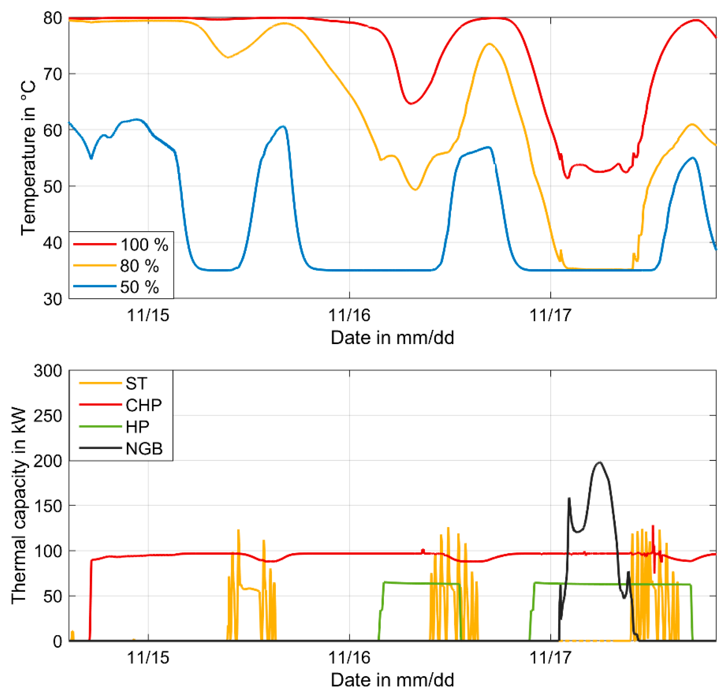
To get an impression of the prediction quality of the models, Figure 6 shows the prediction of the uppermost storage tank temperature as the most important temperature to be predicted over a period of one day as well as the distribution of the prediction error in the range below 61 °C, which is particularly relevant for operation, for one year.

The distribution of the prediction errors is additionally shown for data that do not include the first 30 days, i.e., the learning phase of the optimizer. For the comparison, prediction horizons of 24, 12, 6 and 3 h were used. The differences to the results of the simulation described in Section 3 are shown as “errors”. Boxplots like the two right graphs in Figure 6 summarize statistical dispersion and location parameters in one plot. The median of the prediction error is marked as a horizontal line in the boxes, the range of values between the 25 and 75 percentile is marked as a box (=interquartile distance). The whiskers show the range of 1.5 times the interquartile distance. All values outside this distance are defined as outliers and are marked as red crosses.

The exemplary course of simulated storage temperature and the associated predictions show that a reasonable prediction can be made with the GPR models, considering the large number of sources of error. The consideration of the distribution of the errors clearly shows that the distribution becomes narrower with a decreasing prediction horizon. Also, the errors are quite small for most of the time steps. Taking the example of the prediction with a 24-h prediction horizon, the median error is −0.05 K with a standard deviation of ±0.6 K (approx. 2.3% relative deviation with respect to the mean value of the temperature in this range). High errors can have a variety of reasons, but especially the low data availability at the beginning of the predictions at the beginning of the year and the reduced amount of data for training due to the selection algorithm. If the first 30 days (training phase) are not considered, the distribution of the prediction errors becomes narrower. The relative standard deviation in the case of the 24 h prediction is reduced from 2.3 to 1.9%.

To get a further impression of the prediction quality of the models, Figure 7 also shows the prediction of the further temperature layers for an exemplary section, in all cases with a prediction horizon of 12 h.

The effects of the storage temperature prediction on the prediction of the boiler power as well as the final calculation of the target values are shown in the next section.

4.3. Boiler Power and End Energy Usage Approximation

Figure 8 visualizes the boiler power over the average heat load as well as the uppermost storage temperature at the end of a time interval. The data are taken from a yearly simulation where random settings of the controllable variables were made.

The mean boiler power (and conversely, inversely proportional to the storage power) behaves nonlinear. As the upper storage temperature rises, the required boiler power decreases to 0 kW, where it remains even if the storage temperature continues to rise. Below the grid temperature of 55 °C, more boiler power is required, depending on the heat output of the CHP and HP as well as the storage temperature and the heat load.

Using a similar meta-heuristic approach as mentioned in the last subchapter, it was found that the approximation of the average storage power in the next time interval and, analogously, the predicted power of the boiler ${\widehat{Q}}_{NGB}$ (cf. Equation (5)) can be described via a linear regression including interactions. Equation (10) shows the general function whose regression coefficients are determined using the Least-Square method:

$$\begin{array}{c}{\widehat{Q}}_{NGB}=\{\begin{array}{c}{b}_0+{\displaystyle {\displaystyle \sum }_{j=1}^{j=n}}{b}_j{x}_j+{\displaystyle {\displaystyle \sum }_{j=1}^{j=n-1}}{\displaystyle {\displaystyle \sum }_{k=j+1}^{k=n}}{b}_{j,k}{x}_j{x}_k, T_{TS,t+1,4}<61\mathrm{deg}\mathrm{C}\\ 0,T_{TS,t+1,4}\ge 61\mathrm{deg}\mathrm{C}\end{array}\\ n=Number of Factors\\ x=Normalized Factor Setting\\ b=Regression Coefficient in \mathrm{kW}\\ T_{TS,t+1,4}=Upper Storage Temperature in \mathrm{deg}\mathrm{C}\end{array}$$

(10)

In contrast to the prediction of the storage temperatures, the boiler performance is not a self-dependent prediction. Also, the use of simple regressions allows the use of a larger data set without time criticality, therefore the selection of data shown in Section 4.3 is not necessary here.

Figure 9 shows, analogous to Figure 6, the course of the boiler performance prediction for one day and the distribution of the absolute prediction errors for different prediction horizons, whereas the storage temperatures required for the prediction (cf. Equation (5)) again come from the models described in Section 4.3. Most of the errors are quite small. Single large outliers can be mainly due to the erroneous predictions of storage temperatures and the inaccuracies of the linearized model. For the prediction with a horizon of 24 h the median of the prediction error is 0 kW with a standard deviation of ±4.7 kW, without the first 30 days the standard deviation is reduced to ±4.2 kW.

Like the boiler performance prediction, classical databased regression functions can be used for secondary energy predictions (gas consumption of CHP and boiler, electricity production of the CHP and electricity consumption of the WP, see Equation (4)). The resulting operating costs and CO₂ emissions can be calculated using completely defined, functional relationships. Figure 10 shows the observed over the predicted sum of operating costs and CO₂ emissions for different prediction horizons. The additionally given coefficient of determination R² as a quantitative evaluation criterion shows the percentage of explained variance in the total variance.

All plots show that the prediction of the sum of operating costs and CO₂ emissions works very well. The individual prediction errors of the underlying models partially balance each other out over the prediction horizon. A longer prediction horizon leads to a better balance and thus to a higher degree of certainty. Whether the achieved prediction quality is sufficient to enable a meaningful optimization is discussed in Section 6.

4.4. Implementation in Simulation Environment

To use the approximations for an optimization, the data generation and multi-stage modeling (see Section 4.2 and Section 4.3) must be combined with an optimization algorithm. For the multi-objective optimization, here of operating costs and CO₂ emissions, the use of a multi-swarm optimization (as developed by Coello Coello and Lechuga [29]) has proven to be performant. Several basic populations are moved through a search space by passing on the information of non-dominated individuals, whereby different approaches are used to reduce getting stuck in a local optimum. It is shown that especially by vectorizing the properties of the considered individuals or by parallelizing the evaluation of the functional relationships a solution can be found in a sufficiently fast time (here in less than 30 s).

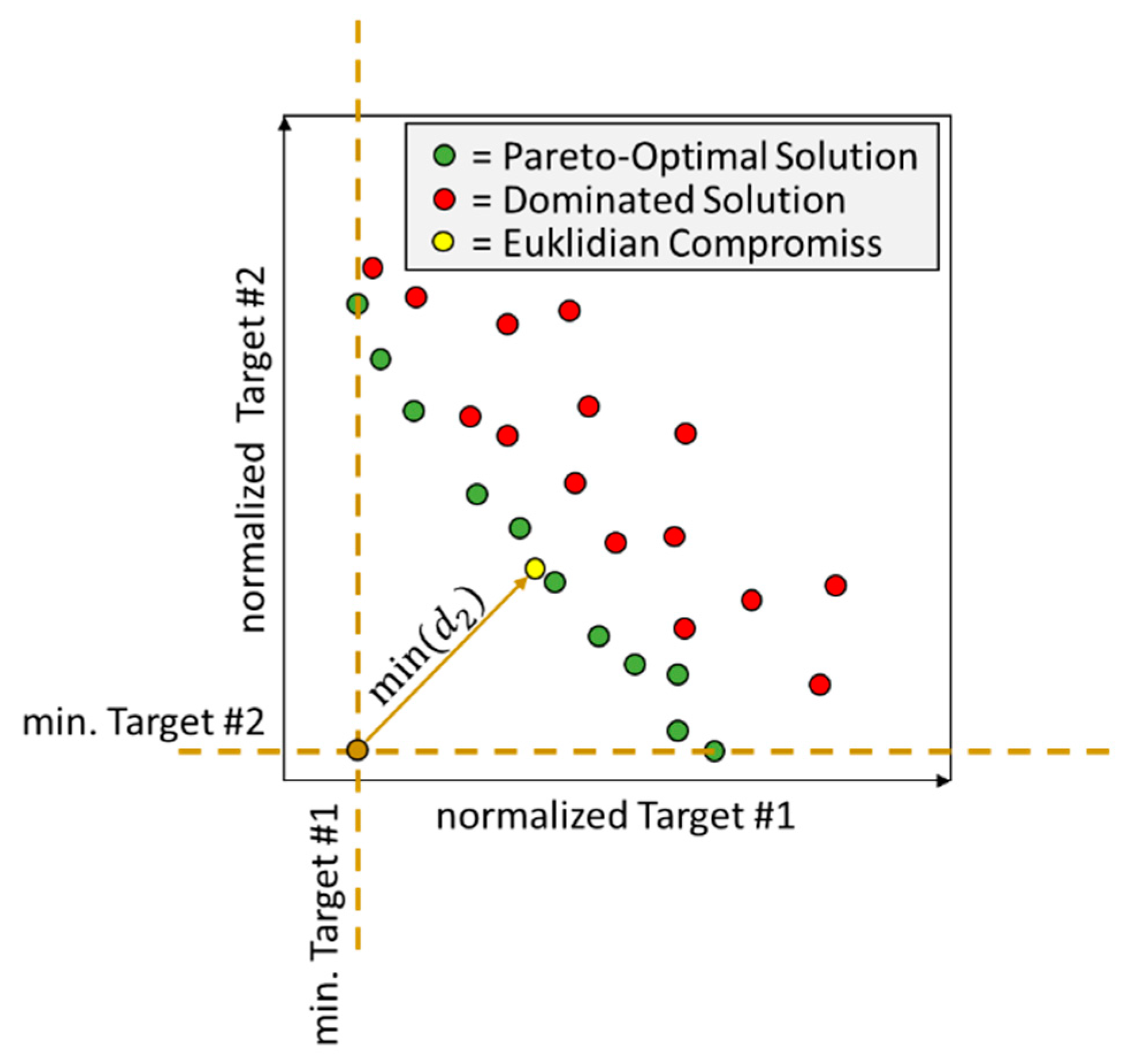
In order that the optimization of the operation can take place without user intervention, an automated evaluation of the non-dominated or pareto-optimal solutions must be performed in the multi-objective search space. In this work, the Euclidean distance $d_2$ of the pareto-optimal solutions $y_{po}$ to the theoretical optimum $y_{to}$ is calculated (see Equation (11)). The theoretical optimum is initially approximated by scanning the design space by an equally distributed experimental design (see Ye [30] for more details):

$$d_2\left(y_{to},y_{po}\right)=\sqrt{{\displaystyle {\displaystyle \sum }_{k=1}^2}{\left|y_{to,k}-y_{po,k}\right|}^2}$$

(11)

Figure 11 shows the exemplary, abstracted result of a multi-swarm optimization, including selection of the pareto-optimal solution with the smallest Euclidean distance to the theoretical optimum as best compromise of the achievable target values

The optimization starts in the simulation environment after two simulated days, because then a first databased training of the approximation models is possible. The prediction horizon (e.g., 24 h) as well as the target variables to be optimized are freely selectable at the beginning. Every hour, the different approximation models are created based on the generated data and the optimization or minimization of the target value(s) in the prediction horizon is performed. As a result, the settings of the controllable variables (average power of CHP and HP) for the next time interval, i.e., for the next hour, are transmitted to the control system of the dynamic simulation. After another simulated hour, the new data points are added to the data pool for the formation of the approximation models and the optimization starts again.

For the optimization, additional boundary conditions are considered. For example, CHP and HP are not operated if the inlet temperature to these units is too high. Start-up processes that limit or reduce the output power are also considered.

To evaluate the operational optimization, the difference between the cumulated targets of the reference and the optimization is calculated:

$$\begin{array}{c}\mathrm{dK}={\displaystyle {\displaystyle \sum }_{t=1}^{t_{max}}}{K}_{ref,t}-K_{opt,t}\\ t_{max}=Number of considered time steps\\ K_{ref,t}=Costs of Operation for time step t with standard controller\\ K_{opt,t}=Costs of Operation for time step t with optimization\end{array}$$

(12)

$$\begin{array}{c}\mathrm{dE}={\displaystyle {\displaystyle \sum }_{t=1}^{t_{max}}}{E}_{ref,t}-E_{opt,t}\\ E_{ref,t}=C{O}_2-Emissions for time step t with standard controller\\ E_{opt,t}=C{O}_2-Emissions for time step t with optimization\end{array}$$

(13)

5. Description of Relevant Data and Scenarios

An economic and ecological evaluation of plant operation always depends on the applicable energy-economic and political framework conditions. For example, the plant described in Section 3 benefits from the current German policy of promoting the maintenance, modernization and expansion of combined heat and power generation, recorded in the so-called KWKG [31]. The KWKG creates favorable economic conditions for the operation of a CHP plant by applying a preferential tax rate to fossil fuels and paying a performance-related surcharge for a limited period per kilowatt-hour of electricity generated. The ecological assessment benefits from the so-called electricity credit method [32]. With this method, it is assumed that the amount of electricity generated by the cogeneration plant will mainly displace electricity from hard coal-fired power plants, where emissions and primary energy are saved. The CHP plant receives these savings as a credit on the emissions released during its own operation or on the primary energy used which means that emissions and primary energy use of the CHP plant are reduced to below zero, especially at high electrical efficiencies. According to the Building Energy Act (GEG) [33], which has been in force in Germany since November 2020, operators of CHP plants may only give a value of zero as the lowest value for emissions and a value of 0.3 for the primary energy factor (= primary energy used/heat output) (up to 0.2 for 100% renewable primary energy). Due to the aspects described, CHP plants, especially those with high electrical efficiencies, are currently strongly favored in Germany, both economically and ecologically. Only in times of negative electricity prices below about minus 10 €/MWh does an electrically driven heat pump achieve lower heat generation costs than a CHP plant, since no surcharges are paid for the CHP electricity in such times. These energy-political boundary conditions, which are valid today, are included in scenario 1.

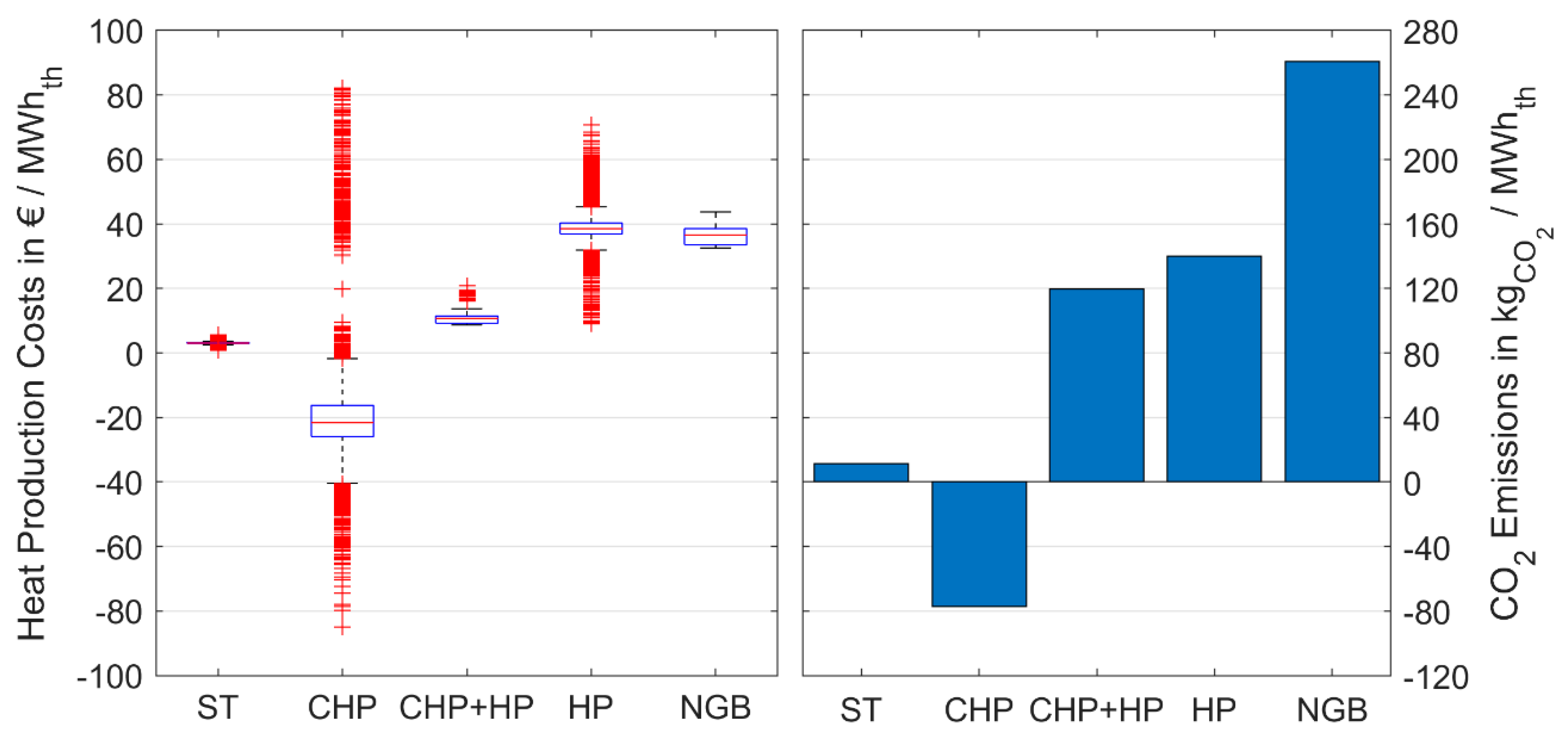
For the 2017 and 2018 period under consideration, Figure 12 shows the theoretical heat production costs including all subsidies, taxes and charges in Germany as a function of the actual exchange price for electricity and gas for the German energy market for various heat generators as a box plot. In addition to the boxplots, the emission factors of the heat generators are shown. Since the specific emission factors per kWh of consumed secondary energy are fixed and constant in the JIT, the emission factors of the heat generators (=emission per kWh of heat emitted) are not subject to any fluctuation at constant assumed efficiencies.

The median values of the heat production costs show that, apart from the feed-in priority of the solar thermal plant (ST), the simple switch-on sequence of the heat generators according to the model in Section 3 represents the most economical and ecological operation for the predominant time of the year under the currently prevailing boundary conditions. The red crosses in the figure indicate outliers in the costs, which are due to a strong variability of electricity and gas prices on the stock exchange. In the case of the CHP plant, the outliers above 20 €/MWh_th mean negative electricity prices and thus the omission of the surcharges paid under the KWKG. At the same time, the heat production costs of the heat pump sink by the negative electricity prices, whereby it would be more economical, but not more ecological in these few hours in the comparison scenario to deviate from the classical switch-on sequence and to operate the heat pump instead of the CHP plant. The optimizing regulation should recognize this and switch the heat generators accordingly. In times of high electricity prices, the heat production costs of the heat pump are higher than those of the gas boiler. However, since the combination of CHP system and heat pump is always cheaper than boiler operation, the boiler will not be preferred. In principle, it is to be expected that the optimizing control system will strive for the highest possible number of operating hours of the CHP system due to the electricity credit method and thus even cause a displacement of the solar thermal system compared to the standard control system. Due to the low heat load in summer, however, only small displacement effects, if any, are to be expected.

The expansion targets for CHP in Germany laid down out the KWKG have almost been reached and subsidies are expected to expire in a few years. Although the electricity credit method described above has already been modified in the Building Energy Act, in comparison with the previous regulation in the direction of a worse rating of CHP plants and a better rating of combined HP and CHP, it is still unchanged until at least 2030. The second scenario roughly reflects the framework conditions to be expected in the next 10 years (see Figure 13): Sale of the produced CHP electricity at the stock exchange price without surcharges from the KWKG but continued ecological improvement by crediting avoided CO₂ emissions as is currently the case.

Compared to the first scenario, the heat production costs of the CHP plant show less variability due to the elimination of surcharges under the KWKG and the pure coupling of electricity revenues to electricity exchange prices. In comparison to Figure 14, this can be seen in the shift of the boxplot in the amount of the unpaid CHP surcharges. In terms of economics, the standard regulation with fixed switch-on sequence is now more often at a disadvantage compared to heat pump operation due to the increased costs of CHP operation. Although scenario 2 offers a larger number of hours with optimization potential compared to scenario 1, the absolute improvement potential of these hours is much smaller due to the now smaller cost gap between the units. Due to the forward-looking character of the optimizing control, it can be expected that the operating times of the heat generators will be shifted to times with lower costs (with low gas/electricity purchase prices) and high electricity revenues (with high electricity prices; applies only to CHP). Due to the identical emission factors but changed costs compared to the first scenario, the second scenario is particularly interesting for multi-criteria optimization. There is a field of tension between the temporarily higher costs of the CHP plant and at the same time lowest emissions compared to the other heat generators.

Scenario 3 differs from the second scenario only in the calculation of CO₂ emissions. The so-called Carnot method, also known as the work value method as detailed by Veigel [34], divides the emissions of the fuel used into the co-products heat and electricity depending on the respective exergy. The CO₂ emissions caused by the production of heat and electricity are shown separately, whereby only the emissions from heat production are relevant here.

In all scenarios, it is important to note that for the purchase and sale of electricity on the stock exchange, the electricity volumes for trading must be known in advance and must be fed or consumed appropriately. Both requirements depend largely on the prediction quality of the models.

6. Results and Discussion

In the following, the results of the optimization, influenced by the beforehand mentioned scenarios, are presented and discussed. For the optimization, the multi-stage approximation with a prediction horizon of 12 h, as shown in Section 4, is used. As a benchmark for the evaluation of the optimization results the results of the standard control described in Section 3 are used. The simulation starts on January 1, 2017 and ends 500 days later.

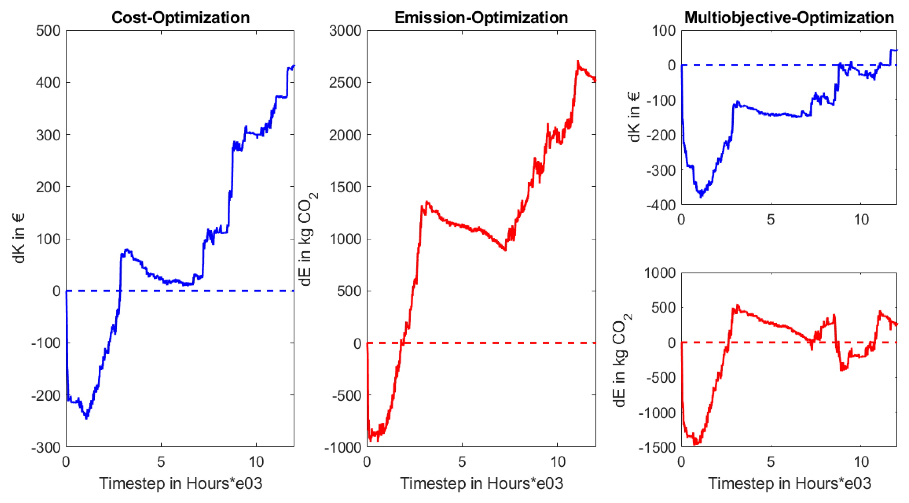
Figure 15 shows the optimization results influenced by the boundary conditions of scenario 1, on the left for the cumulated costs $dK$ with pure cost optimization, in the middle for the cumulated CO₂ emissions $dE$ with pure CO₂ emission optimization and on the right for both cumulated target variables with multi-objective optimization. The horizontal, dashed line shows the zero line in each case. If $dK$ or $dE$ are above this line, the optimizer delivers a better value of the respective target quantity cumulated up to this time step than in the reference simulation with standard control.

For all optimization targets, the optimizer achieves a result above the dashed zero line at the end of the simulation period, i.e., a better result than the standard control. In the initial phase, the optimizer makes disadvantageous decisions. Only after about 1000 h improvements occur, which is understandably related to the growing data basis for the approximation models. In the heating periods, especially in the second with now well-trained approximation models for the storage temperatures, a positive slope of the curve progressions (optimizer is better than the standard controller is) tends to be visible. In the summer months, the optimizer loses slightly compared to the reference simulation. The reason might be that the storage temperatures are predicted too high if the performance of the solar thermal system is overestimated. Both reduce the ecologically and economically advantageous CHP operation in scenario 1. The purely temperature-controlled reference system does not have this problem, as it prioritizes the CHP plant from the switch-on sequence independent of future prediction.

Table 3. Optimization results of scenario #1 in comparison to the results with standard controller.

Optimization-Goal	$\mathit{r}\mathit{T}$ in % (Costs/CO2)	$\mathit{r}{\mathit{T}}_{30}$ in % (Costs/CO2)
Cost of Operation	+10.7/−123.6	+16.1/−43.9
CO2-Emissions	−25.9/+197.3	−17.8/+263.5
Multi-objective	+1.1/+21.7	+9.5/+136.4

summarizes the results of the optimization at the end of the period. For this, the relative change in cumulated target values compared to the standard control over the entire period ($rT$) as well as for a period without the first 30 days ($r{T}_{30}$) is shown.

In the case of the optimization of the operating costs a reduction of the energy quantity of the heat pump by approx. 8% and an increase of the energy quantity of the boiler by 8% takes place over the simulation period compared with the standard control. For the optimization of the CO₂ emissions the reduction of the energy quantity of the heat pump amounts to approx. 50% and the increase of the energy quantity of the boiler approx. 48%. This is because the heat pump can only be operated at 50% or 100% of the maximum power, whereas the boiler has no lower modulation limit in the simulation. At times when the heat load is above the maximum CHP power but below certain combinations of combined power of CHP and HP, it may be better to operate the boiler at the appropriate output than to request too much heat pump power. To optimize costs, however, there are also individual hours per year during which the boundary conditions speak for additional operation of the heat pump (e.g., in times of negative electricity prices). This does not apply however to the optimization of the CO₂ emissions, which explains the stronger reduction in the energy quantities. For the multi-objective optimization, a compromise is found, which ensures that both targets exhibit a positive difference to the reference. It can be stated that the implemented MPC finds a significant improvement to the reference for all cases.

In scenario 2 there is no additional compensation for the electricity generated by the CHP. The specific CO₂ emissions remain unchanged compared to scenario 1. For this reason, only the optimization of costs is considered in Figure 16.

The almost consistently positive gradient of the difference in cumulative operating costs makes it clear that, analogous to scenario 1, cost optimization is very well possible. Even the summer months no longer have a negative effect on optimization. This is because, in contrast to scenario 1, it is now not always advantageous to operate CHP. Because of the abolition of CHP remuneration, the distributions of the specific heat production costs converge (see Figure 13), which means that operating CHP is more often uneconomical. Although this increases the number of points in time when optimization is possible, it reduces the potential benefit per optimization. In sum,

Table 4. Optimization results of scenario 2 in comparison to the results with standard controller.

Optimization-Goal	$\mathit{r}\mathit{T}$ in % (Costs/CO2)	$\mathit{r}{\mathit{T}}_{30}$ in % (Costs/CO2)
Cost of Operation	+5.3/−3703	+5.9/−3516

shows that the relative improvement in operating costs is only about half as great as under scenario 1.

Due to the approx. 20% reduction in the amount of energy produced by the CHP over the simulation period, the electricity credit for emissions drops significantly, with a correspondingly large deterioration in overall CO₂ emissions.

In Scenario 3, the CHP no longer gives an electricity credit for CO₂ emissions. The operating costs do not change compared to scenario 2. For this reason, only the optimization of CO₂ emissions is considered in Figure 17.

Analogous to scenario 2, there is an almost continuous improvement. The loss of the electricity credit reduces the maximum possible improvement through increased CHP operation. Compared to scenario 1, this leads to a much smaller relative improvement (see

Table 5. Optimization results of scenario 3 in comparison to the results with standard controller.

Optimization-Goal	$\mathit{r}\mathit{T}$ in % (Costs/CO2)	$\mathit{r}{\mathit{T}}_{30}$ in % (Costs/CO2)
CO2-Emissions	+1.2/+2.6	+1.6/+3.7

). However, this circumstance also promotes the simultaneous use of CHP and heat pump, which explains a reduction in the amount of energy from the CHP of approx. 3% and an increase in the amount of energy from the heat pump of approx. 8.5%.

The results show that the developed MPC achieves an advantage over a non-predictive standard control for every scenario. Only the learning phase of the multi-stage approximation based on Machine Learning methods reduces the performance. However, the quantity of the improvement depends significantly on the scenario of the energy-economic boundary conditions, which defines the potentials of the optimization. The following section summarizes the results of this work and outlines the potentials as well as further steps.

7. Conclusions and Outlook

7.1. Multi-Stage Approximation for Optimized Control

The operational optimization of the heat generation of multivariate fed local heat networks is a complex problem due to the nonlinear system behavior. This is especially true if the system under consideration has storage with a stratified charging system. Its change of temperature distribution, which is essential for an operation optimization over several hours, is highly nonlinear. The method presented here depicts the nonlinear relationship between the most diverse influencing variables and the ecological and economic target variables of the operation predictively employing a multi-stage approximation, among other things using machine learning methods. This work contributes to the scientific community by: (i) showing a path for use of databased nonlinear metamodeling for efficient operational optimization of district heating networks and (ii) depicting the strong influence of regulatory boundary conditions on the potential of optimization.

The implementation of this operational optimization with a prediction horizon of 12 h into the dynamic simulation of a multivariate fed local heating network shows a significant reduction of operating costs and CO₂ emissions over a simulation period of 500 days for different regulatory conditions compared to a non-predictive standard control. It should be noted that the comparisons made so far assume that external boundary conditions (weather data, stock exchange prices, heat load in the network) are known.

Further work until the implementation of the optimizing controller in the heat center of the new local heating network in mid-2021 will concentrate on the addition of the prediction for the above-mentioned external boundary conditions and the improvement of the approximations concerning prediction quality and computation time. In extension, it is planned to test the integration to the electricity and gas market in the simulation environment. This requires a combination of extensive offline optimization, in which uncertainties of the prediction or the robustness of the operating recommendations are included as a further criterion in the optimizing control, as shown by Reich et al. [35], with online operation optimization, which also takes into account a reduction of balancing energy in the power grid.

7.2. Impact of District Heating Networks on Local Electricity Grids

As the energy transition in Germany progresses, options to stabilise the electricity grid will gain importance. An expansion of the modelling and optimisation approach of this work to include grid-stabilising effects is therefore seen as an important future field of research.

The interaction with the local electricity distribution grid is based on the generator-side power of the CHP plant integrated into the local heating network and the consumer-side power of the heat pump. Theoretically, operation optimised purely to the requirements of the local heating network can lead to grid-related congestion, which in turn must be eliminated by re-dispatching.

In contrast, the thermal inertia of the local heating network and the available heat storage power allow for the inclusion or even active alignment to grid-friendly operation. The multivariate prognosis of the nonlinear system behaviour of the local heating network presented in this work can be extended by optimisation criteria for grid-friendly service, i.e., it can include all network restrictions (security-constrained economic dispatch) as well as possibilities of sector coupling. Aspects relevant for a grid-friendly operation can be unleashed by the avoidance of local grid-related congestion or through incentives for regional pricing. Figure 18 illustrates the modelling approach for a grid-friendly operation of the local heating network, distinguishing between both possibilities.

(i) The influence on the local electricity distribution network is becoming increasingly important, especially when upscaling the local heating network with incorporated sector coupling technologies. Within the framework of future work, the effects of avoiding local grid-related congestion as a restriction in the dynamic optimisation model with real data are very relevant for research. For this purpose, the data-based criteria of the grid situation can be used as additional boundary conditions for operational optimization.

(ii) The current market design, which is based on a uniform electricity price, is only suitable to a limited extent to promote the operation of the local heating network in a grid-friendly way. Modelling of the grid-related potential can be based on the approach also known as “nodal pricing” or “locational marginal pricing (LMP)”. In nodal pricing systems, an individual price is determined for each entry or exit point of the transmission system, thus providing an incentive for grid-friendly service through regional electricity pricing. The operation of all modelled generation and consumption units thus takes place in compliance with the network restrictions, as these restrictions are reflected in the electricity price which is sharply defined at the network nodes. Any use of P2H elements is therefore grid-friendly in the event of local congestion, as grid overload is ruled out by the model. The extent to which regional pricing can stimulate grid-friendly operation and the potential for grid-relief is an addition of the research subject of this paper.