Abstract
During satellite development, engineers need to simulate and understand the satellite’s behavior in orbit and minimize failures or inadequate satellite operation. In this sense, one crucial assessment is the irradiance field, which impacts, for example, the power generation through the photovoltaic cells, as well as rules the satellite’s thermal conditions. This good practice is also valid for CubeSat projects. This paper presents a numerical tool to explore typical irradiation scenarios for CubeSat missions by combining state-of-the-art models. Such a tool can provide the input estimation for software and hardware in the loop analysis for a given initial condition and predict it along with the satellite’s lifespan. Three main models will be considered to estimate the irradiation flux over a CubeSat, namely an orbit, an attitude, and a radiation source model, including solar, albedo, and infrared emitted by the Earth. A case study illustrating the tool’s abilities is presented for a typical CubeSats’ two-line element set (TLE) and five attitudes. Finally, a possible application of the tool as an input to a CubeSat task-scheduling is introduced. The results show that the complete model’s use has considerable differences from the simplified models sometimes used in the literature.
1. Introduction
At present, except for nuclear energy, photovoltaic is the only technology capable of sustaining a satellite’s operation while in orbit [1]. In critical space applications, power prediction and management are essential parameters for mission value extraction and quality-of-service assurance. Even before a satellite leaves the ground, scenarios should be tested to understand the satellite’s behavior in orbit and minimize the occurrence of failures, or possible inadequate operation [2]. These acceptable practices are mostly valid for CubeSat projects, which are satellites of small physical dimensions, generally of low cost, with extensive use of commercial off-the-shelf (COTS) elements, short schedule, short operational lifetime, limited redundancy, and extensive testing focused on system-level [3]. Notice that the limited energy harvesting abilities of CubeSats (due to their small physical dimensions) can impact the real valuable work performed in orbit, which is primarily determined by the scheduling plan [4].
The electronic miniaturization, COTS components for nanosatellites, and the use of a standard platform—the CubeSat—reduced the cost of a satellite project, so universities and companies can afford it [5]. The model 1U is the basic CubeSat geometry, a cube with dimensions of 10 cm, usually covered by photovoltaic panels (PV) on its external surfaces that recharge the batteries and generate the power to operate the sub-systems [6]. The great majority of CubeSats are in Low Earth Orbit (LEO) (nanosats.eu), below 600 km, where the sun is the primary source of energy for the PV, reason for critical dependence of the solar panels’ projections towards it for appropriate energy harvesting [7]. Another critical parameter for satellites’ power system that results from the attitude is the PV and battery’s temperature, limited by a narrow range. Temperature levels beyond the recommended values may permanently damage the satellite, but even deviations from optimum point results in an inefficient operation [8,9,10].
In the work of [11], the authors review the environmental conditions and their impact of typical batteries used in CubeSat missions. For low values of temperature, usually below −20 C and 0 for discharge and charge conditions, respectively, there is a rapid degradation of its performance. The same tendency of low efficiency exists for high values of temperature. The levels of irradiation and its accumulation through the orbit lifetime reduce the battery’s performance, especially when shielding is absent. The work of [12] develop and conduct experimental tests regarding the state-of-charge estimation for the battery of satellites, totally dependent on the power generation capacity of the photovoltaic cells. However, the authors do not assess it considering typical transient irradiance and temperature profiles found in orbit. Thermal simulations of CubeSats are found in [13,14,15,16,17], where the authors solve the transient temperature of critical components of the satellite, like the battery or some electronic component of a payload, to understand if the thermal operational limits of the satellite are satisfied. Concern about temperature also occurs with experimental payloads, such as biological experiments, where a specific range of temperature must be achieved [18,19], or for the design of novelty and optimum CubeSats concepts [20,21].
The irradiance field over a spacecraft is a transient phenomenon, a function of orbital parameters, geometry, attitude, and the calendar [22]. Orbit shape and direction are essential because when the Earth is between the line of sight of the CubeSat and the Sun, there is no solar radiation, which is the main source of radiation. Unless specific conditions are met, the orbit is dynamic, so the date enters the equations to estimate the Earth’s occurrence of shadows. The CubeSat’s attitude, or its orientation, is another significant parameter and expresses which parts are exposed to a particular irradiation source. Therefore, the engineer’s challenge in the determination of the irradiance is the integration of orbit, attitude, and irradiation source into a single model to estimate the worst, best, and intermediate scenarios that the CubeSat will be exposed to in orbit.
A better irradiance estimation is useful for hardware in the loop simulators like the “sun simulator” presented in [23], where the authors connected LEDs to LabView in order to emulate the orbit conditions in their experiments or the procedures to emulate solar panels and batteries described in [24], both focusing on FloripaSat-I. As stated in [25], through the case study of the e-st@r-I CubeSat, hardware in the loop is an important process for verifying the functional requirements of CubeSats. Another example of hardware in the loop approach was implemented in the development of the CubeSat MOVE-II to simulate the space environment in real-time during on-ground tests [26]. Their work emulated a solar array’s electrical behavior through a voltage–current characteristic curve, a function of illumination level and temperature of the photovoltaic cells in the array.
A numerical tool to explore typical irradiation scenarios for CubeSat missions is the main goal of this work. Such a tool can provide the input estimation for software and hardware in the loop analysis for a given initial condition and predict it along with the satellite’s lifespan. Three main models will be developed to estimate the irradiation flux over a CubeSat, namely an orbit, an attitude, and a radiation source model. Thus, the remainder of this paper divides as follows. Section 2 presents a review of the state-of-the-art. Section 3 comprehends the methodology, describing each of the models in detail. Section 4 presents a case study illustrating the tool’s abilities, including scenarios from one typical CubeSats’ TLE (two-line element set) and five attitudes. Section 5 presents possible applications, focusing on offline task scheduling, and the paper closes with final remarks and conclusions in Section 6.
2. Background
A spacecraft design’s dynamic performance should include kinetic, attitude, electrical, thermal, and communication performances, however not all real effects can be included in the system model, and simplifications are introduced [27]. Two areas of great concern in CubeSat applications are power generation and temperature, both closely related to irradiance input. In these two cases, solar radiation is the main source. Due to the distance between the Earth and the Sun, the solar rays are assumed to be parallel when they reach the CubeSat. The recommended value for the flux of radiation by the Sun at the distance of 1 AU (astronomical unit) is W/m, equivalent to a black-body at the effective average temperature of 5500 C, although there are small variations due to the cyclic activity of the Sun every 11 years and the elliptic orbit of the Earth (1322 W/m–1414 W/m) [28]. The solar spectral distribution has a peak around 0.5 m, and the energy distribution is about 7% in the ultraviolet, 46% in the visible, and 47% near IR.
A second important source of irradiation for photovoltaic and thermal problems of CubeSats in LEO is a consequence of the reflection of solar rays by the Earth, called albedo [28]. There is no unique and accurate model valid for satellite applications because it is a function of a great diversity of parameters, as atmospheric conditions, clouds, and the ground surfaces [29,30]. Continental areas have a higher albedo coefficient than the ocean, so do lands covered by snow and sand. The global annual average, widely accepted for satellites in LEO, is [31,32]. The Earth’s surface and atmosphere behave like a Lambertian surface; therefore, the reflected radiation can be represented by a phase function [32], whose reflectance increases with a reduction in the solar elevation angle. In other words, the albedo is maximum below the subsolar point, which is the point on the surface whose Sun is upright, and vanishes at the line between the shined and shadowed sides of the Earth [28,31,33]. The albedo’s spectral distribution has significant variation within 0.29 to 5.00 m [31,34]. After the direct solar radiation, the diffuse albedo radiation is the essential load for a PV, even though there are shifts and gaps in its spectrum compared to the direct solar radiation [35].
Another source of irradiation for satellites in LEO assumed in this work is the infrared radiation emitted from the Earth, useful for thermal problems but neutral for the photovoltaic effect as it is a much longer wavelength than the Sun’s emission (>4 m). Warmer surfaces of the Earth will emit more radiation than colder, but dense clouds can block it before it hits the satellite, reason for significant variations worldwide, although much less severe than albedo [28,31]. This infrared radiation is usually higher near the subsolar point, while it is lower near the poles and at night, a consequence of the surface’s temperature. Although there are these variations, an average and constant value usually assumed in the literature is a flux of W/m based on the effective average temperature of −18 C for the Earth’s surface [28,31]. In this context, another final irradiation is from the cosmic microwave background, corresponding to black-body radiation at 2.7 K, although its magnitude is minuscule compared to the previous sources mentioned above. By modeling these radiation sources, traditional big and nanosatellites are thermally tested. For example, the Chinese GF-4 satellite had a difference between the predicted and measured temperatures around 3 C for most of the components [36]. FloripaSat-I [13], PiCPoT [14], UoMBSat-1 [15], and SMOG-1 [17] are examples of CubeSat missions with thermal simulations.
One preliminary way to visualize the general radiation environment that a satellite in orbit is exposed to can be done through the orbit angle, which defines the minimum angle between the orbit plane and the solar vector [28], as shown in Figure 1.
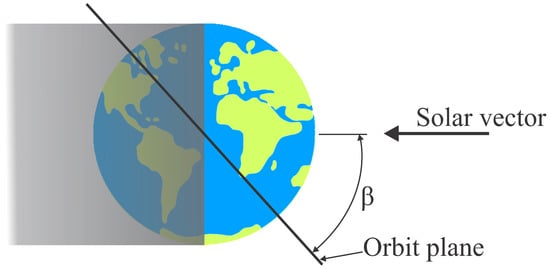
Figure 1.
The angle.
For an angle , the orbit has the longest eclipse caused by the Earth, and the albedo is maximum whenever the satellite passes below the subsolar point. For any value different than 0, the eclipse is shorter, the peak of albedo reduces, and, as increases, the eclipse decreases until a point where it vanishes, depending on the altitude. At exactly , the albedo is null. Therefore, a high value for may be interesting for the photovoltaic cells; however, it may not be in terms of heat transfer if the satellite must be kept at low temperatures. is nearly constant along the months only for sun-synchronous orbit, a special case where, for satellites in LEO, the orbit inclination is very high, around 98. Over several months, to keep a constant angle requires the use of thrusters in the spacecraft to counterbalance the perturbations of the orbit. For the remaining cases, we expected a significant variation of within days, but limited to , where is the ecliptic and i the orbit inclination. Therefore, it is important to recognize that the CubeSat’s missions may be exposed to different , so it is indispensable to understand the orbit behavior to predict the satellite’s future positions. The importance of the parameter with the irradiation sources cited above has already been used for temperature estimation, and comparison with experimental temperature data of the International Space Station (ISS), obtaining good consistency of the results [37]. The CubeSat CIIIASat also presents temperature results and its relation with [38].
Fundamental is also to inform the initial state. It is common to use the standard Two-Line Elements (TLE), which comprehends a set of orbital parameters obtained from satellite-tracking observations, for example, available at the CelesTrak database (www.celestrak.com). The CelesTrak database is a useful platform to initialize orbit simulations with real input if the user wishes to run real orbit conditions. In its catalog, the user can find the TLE of more than 16,000 objects, including CubeSats and their historical data [39]. The use of TLE is encouraged because it is open-access and worldwide spread. Nevertheless, it is valid to mention that the TLE is a picture of the current orbit and is not valid for future orbits due to the natural perturbations presented in every orbit.
The real trajectory of a satellite does not strictly follow the two-body problem theory, which is based in the Keplerian motion. In more or less sense, every orbit is subject to perturbations, which is the effect that causes the deviation from the Keplerian orbit. The non-spherical central body, atmospheric drag, solar radiation pressure, thrust, and gravitational interactions with celestial bodies are the most common perturbations for the orbit. For satellites in LEO, especially below 600 km, which is the majority of the CubeSat missions, the main perturbations are originated from the atmospheric drag and gravitational perturbations, this last one more evidenced by the term J2 [40,41].
The space environment is not a perfect vacuum. Eventually, the satellite will hit molecules of gas, which will decrease its velocity and retard the satellite’s motion [42]. The probability of hitting these molecules decreases with the altitude, but it is not zero. The density of the atmosphere is around kg/m at 100 km of altitude, a reference value where space begins and decreases to kg/m at 400 km, which is close to the altitude of the ISS [40]. As a consequence of this drag, elliptic orbits circularize, the angular momentum decreases, and so does the orbit altitude until the satellite reenters the atmosphere if no booster acts. Atmospheric density is a critical factor for correctly predicting this perturbing force [39,43], which is a reason for a great variety of models with diverse accuracy and computational costs in the literature. The models from the families Jacchia, MSIS, and DTM are usually preferred because they bring better relations of accuracy and computational cost [44], notably NRLMSISE-00 [45].
The Earth does not have perfect mass distribution, neither is it a perfect sphere [40]. For these reasons, the gravitational field varies with latitude, longitude, and radius. Due to the oblateness of the Earth (radius at the equator is bigger than in the poles), the right ascension angle (), and the argument of perigee () of an orbit suffer significant variation with time. This feature is taken advantage of by satellites to work in specific orbit inclination (i), as the sun-synchronous () and Molniya (). The equation to describe this perturbation is given by an infinite series, which depends on zonal harmonics (Jk) of the Earth and Legendre polynomials. The zonal harmonic J2 is the biggest one, and it is usually the only term considered in the simulations without significant loss of accuracy. This perturbation’s primary effect is the precession of of an elliptic orbit [39].
One last parameter of concern and fundamental for irradiance analysis is the satellite’s attitude. Issues related to communication, thermal control, and power generation are all impacted by a satellite’s dynamic in orbit. When dealing with small satellites as CubeSats, this becomes more critical as the available space to comport typical engineering solutions is very small, as the available external area for photovoltaic cells [13]. Usually, publications without the focus on control theory idealize the spin of a CubeSat only in a single axis, generally with one face towards the Earth, with an attitude model not versatile enough to reproduce different scenarios [17,46,47,48,49]. The researchers who deal with attitude control use different approaches to describe the satellite’s rotation, as Euler angles, quaternions, and Direction Cosine Matrix [50,51,52]. Euler angles are more intuitive to visualize than quaternion or DCM, but quaternion is the only free of singularities.
3. Methodology
The methodology to estimate the transient irradiance field of this work bases on:
- an algorithm to estimate the orbit of a satellite and its position, valid for elliptical and circular orbits subject to perturbations caused by the atmospheric drag and the effect of the Earth oblateness, available at [40];
- a simplified algorithm developed by the authors herein to mimic the attitude of the satellite;
- a model to project the surfaces of a CubeSat towards the irradiance sources, namely solar, albedo, and infrared radiation of the Earth.
Therefore, this problem will be described by three main models to be further detailed in the next section: Orbit, Attitude, and Irradiation source.
3.1. Orbit Model
The objective here is to estimate the position of the CubeSat in orbit. A generic view of a CubeSat is shown in Figure 2 with some of the parameters required to define it completely.
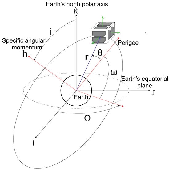
Figure 2.
The orbit and position of a CubeSat.
The constants of the model are:
- Earth’s gravitational parameter: km/s;
- Earth’s radius: km;
- Second zonal harmonics J2 [-].
To initiate the simulation, the first thing needed is the vector of Classical Orbital Elements (COE) [,,,,,], where the subscript 0 means the value at the beginning of the simulation . To obtain the COE at , the algorithm will rely on TLE data so that the user can test with real CubeSat’s orbit information. However, only six parameters from the whole TLE will have to be declared by the user, namely:
- i: orbit inclination [];
- : right ascension of the ascending node [];
- e: eccentricity [-];
- : argument of perigee [];
- M: mean anomaly [];
- n: mean motion [rev/day];
The specific angular momentum (h [km/s]) and the true anomaly ( [rad]) are not readily available from TLE, so they are calculated by Equations (1)–(4), where a is the semimajor axis [km] and E is the eccentric anomaly [rad] [40].
It is crucial to transform the mean motion units to rad/s and all the angles to radians. The eccentric anomaly is solved by some iterative method, for example, the Newton–Raphson. The user also has to inform the day, month, and year in the beginning of the simulation to estimate Sun’s position, as will be shown later.
To find the position of the CubeSat in orbit, we are going to use two reference frames. The inertial Cartesian reference frame, called the geocentric equatorial frame, shown in Figure 2, is defined in terms of the right-handed triad unitary vector [] and located at the center of the Earth. The component points to the vernal equinox direction, is the axis of rotation of the Earth, while is orthogonal to them and forms the Earth’s equatorial plane.
The second reference frame is the perifocal frame of reference, not shown in Figure 2. It is fixed in space, centered at the focus of the orbit and defined by []. points to the periapsis (nearest point of the orbit to the Earth), is 90 true anomaly from the periapsis, and is normal to the plane of the orbit. The true anomaly is measured from this axis of the perifocal frame of reference. The radius (r) of a CubeSat in the perifocal frame of reference may be expressed as:
The transformation from the geocentric equatorial frame into the perifocal frame is done by the classical Euler sequence shown in Equation (6).
The angles , and i are known as the Euler angles, and the matrices in previous equation are:
The matrix in Equation (6) is orthogonal, so the position of the CubeSat in the equatorial frame may be finally calculated by:
The initial position of the satellite can be already found with the TLE input. For an ideal orbit without perturbation, the user would utilize a timestep, the information of mean motion (n) and the mean anomaly (M) to find the next true anomaly (), then the position of the CubeSat. However, for the case with perturbation, there are few more steps in this process.
Equation (9) is valid for the motion in an inertial reference frame with the presence of perturbation (), where the first term on the right side originates from the Keplerian orbit while the second is the perturbation. Ignoring the second term gives the origin of the ideal motion without perturbation briefly discussed above.
Before introducing more equations, a new reference frame is used, called local vertical/local horizontal (LVLH). It is non-inertial, represented by the triad []. is the unit vector of and follows the position of the satellite in orbit, is the same of the perifocal frame, therefore normal to the orbit plane, and is the resulting cross product between these vectors. The components of a perturbation force in the LVLH reference frame are given by Equation (10).
The perturbing forces considered in this work will be the drag and the gravitational perturbation J2 because the cases to be studied here are below 500 km of altitude, a region where these forces are of greater magnitude. Their components will relate to the Equation (10) through:
3.1.1. Drag
The drag () is a force acting opposite to the satellite’s velocity . If we ignore the velocity of the atmosphere due to the rotation of the Earth, we can write:
where is the atmospheric density, is the dimensionless drag coefficient, and A is the satellite’s frontal area. Usually, for is assumed the constant value of 2.2 over the entire orbital lifetime, though the theory agrees it is variable [39]. Dividing the previous equation by the mass of the spacecraft, the drag acceleration is:
where the parameter between parenthesis is also recognized as the ballistic coefficient.
The components of a perturbation with magnitude aligned with the velocity vector of the satellite in the LVLH reference frame are [40]:
Recognizing that the drag perturbation is also tangent to the orbit and opposite to the velocity vector, the parameter is:
where the magnitude of the velocity is [40]:
Therefore, the components of the drag perturbation in the LVLH are:
3.1.2. Gravitational Perturbation
The components of the J2 gravitational perturbation in the LVLH components are given by Equation (18). Further details can be found in [40].
3.2. Gauss’s Variational Equations
The model used in this work for the dynamic behavior of the Classical Orbital Elements bases on Gauss’s variational equations [40,53]. The development can be found in [40], and basically consists of obtaining the COE from the state-vector and then finding the rates. The equations are:
Notice that singularities arise when or , the consequence of assuming that the position vector used in the above equations is the solution of an elliptic orbit [54].
The orbit model is a problem of initial value, essentially summarized by Equations (5), (6), (8) and (19), whose ordinary differential equations of COE are of first order. Therefore, we can write:
where and are the COE vector and its derivative, respectively. The COE at the initial time () is given by the user, as explained previously. The user still has to inform the timestep () between iterations and the final time () of the simulation.
Define the Position of the Sun
Before proceeding to the attitude model, we are going to calculate the sun’s position. It does not impact orbit determination, but it will be necessary to define specific attitudes and compute the eclipse caused by the Earth. To compute the solar vector , we use the following equations, available at [40].
Initially compute the Julian day number () using the date input, where y, m, d and stand for year, month, day, and the universal time of the initial of the simulation. The next equation gives the number of days since J2000 (). and are the mean anomaly and mean longitude of the sun, respectively. is the ecliptic longitude, is the obliquity. Finally, is the unit vector from the Earth to the sun, and the magnitude of the distance is , where km is the astronomical distance.
3.3. Attitude Model
The attitude model aims to mimic the rotation of the satellite around its axis. For a typical CubeSat 1U, without deployable solar panels, there are six normal that describe the orientation of each side k.
In this work, the initial orientations of these surfaces in the perifocal frame of reference are:
To define the attitude, the user will have to write the rotation matrices, which are functions of an angle and axis of rotation, and combine them for different scenarios. The initial set of rotations are executed in the perifocal frame of reference and, if necessary, later translated to the geocentric frame of reference. For all of them, means the final orientation of surface k after all the rotations performed at instant t, in the geocentric reference frame. Some examples to be explored and discussed in this work are illustrated in Figure 3.
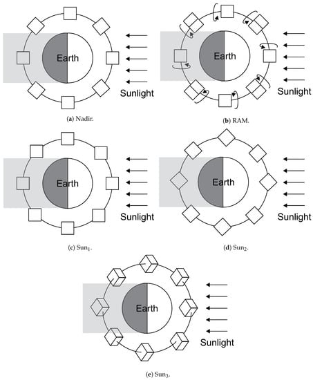
Figure 3.
Attitude scenarios.
Exactly these specific attitudes are difficult to obtain without a precise active attitude control, but yet they are close to typical operation modes as Earth imaging missions, reduced tumbling rate along one major axis, or safe modes where one or more solar panels are exposed to the sun for battery’s recharge [55,56].
3.3.1. Nadir
In this case, the satellite always keeps the same attitude towards the Earth’s center (Figure 3a). For this case, the satellite only rotates around the axis, whose angle of rotation is the same as the true anomaly :
Therefore, as the satellite must follow the orbit inclination, it is necessary to transform from the perifocal to the geocentric reference frame:
3.3.2. RAM
Another example with the nadir matrix is the RAM attitude (Figure 3b). In this case, the satellite keeps one of its axis aligned with the satellite’s velocity vector, or in other words, it will rotate around the axis once per orbit, as in the nadir attitude. If the satellite has a residual angular speed Θ along its velocity vector, the resulting rotation matrix is:
Again, the satellite must follow the orbit inclination, so:
3.3.3. Sun-Fixed
Another option is to keep the attitude fixed in the space, for example, towards the Sun, an important case to maximize the photovoltaic energy generation through solar panels of the satellite. In this case, diverse scenarios may be interesting. For example, only one side of the CubeSat (Sun1), two (Sun2) or three (Sun3) equally exposed to the sun, as shown in Figure 3c–e, respectively. For all of these scenarios, the rotation matrix is constant, and the transformation from the perifocal to the geocentric reference frame is not necessary.
The first step is to find a unitary vector perpendicular to the Sun, in the Earth’s equatorial plane, by performing a rotation of components , (Equation (21)) and around the axis, resulting in the vector . After that, the CubeSat’s normal vectors are rotated around the by the angle through the formulation of a rotation matrix around an arbitrary axis [13]:
The first part on the right side is the angle between the solar vector and the axis to place the sides of the CubeSat parallel to the Earth’s equatorial plane. The second term () tilts the CubeSat even more if the user wants to. The following step is to rotate the CubeSat’s normal around the axis and angle to orientate it towards the sun. The angle is between axis and :
Finally, the last rotation will be around the axis, by the angle . The above procedure will result in one face towards the sun, two equally projected or three equally projected, valid for the attitude here called Sun1, Sun2 and Sun3, respectively, as shown in Figure 3. The values for and in each condition are:
- Sun1: , ;
- Sun2: , ;
- Sun3: , ;
3.4. Irradiance Source Model
For CubeSats in LEO, the main irradiance sources are from the sun (), the albedo (), and the Earth () [28].
The solar irradiance reaching the external surfaces k of the CubeSat is:
The parameter is the solar flux (1367 ), is the area of the surface k, is the view factor of surface k towards the sun, and is a variable to express the shadow of the earth. The dot product estimates the view factor:
To compute the shadow of the Earth, one initial task is to locate the sun’s vector (), already performed in Equation (21). Once the sun’s vector is determined, Equation (31) is used to verify if the CubeSat is under the Earth’s shadow, based on Figure 4. Notice the shadow is assumed to have a cylindrical shape.
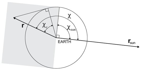
Figure 4.
Diagram to estimate the shadow.
The equation for the albedo irradiation is:
is the view factor of surface k towards the Earth, calculated by [57] and based on Figure 5.
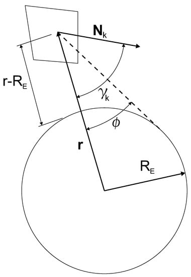
Figure 5.
Geometry to estimate .
The parameter in Equation (32) models the reflection of the solar rays by the Earth’s surface. It is assumed a constant value of for the albedo coefficient, and a cosine function to deliver maximum albedo load when the CubeSat is above the subsolar point, and zero when it passes to the Earth’s side without direct solar illumination, as summarized by Equation (34).
The other source of irradiation comes from the Earth, calculated by Equation (35), where is the solar flux from the Earth (237 W/m).
Therefore, the sum of all main irradiation is:
To summarize, the procedure explained in this work is dedicated to the following scenarios:
- Orbit around the Earth;
- Non-circular and non-equatorial orbits;
- Orbits in LEO, below 600 km, since only the drag and gravitational perturbations are assumed;
- Constant ballistic coefficient;
- CubeSat geometry of any size, without deployable parts.
Before we proceed to the results, a set of equations will be briefly introduced to support the outcomes.
3.4.1. Temperature
In steady-state condition, the thermal balance over a satellite represented by a single node is [13]:
where is the absorptivity of the surface, is the emissivity, is the Stefan–Boltzmann constant, A is the external surface area, T is the absolute temperature, and is the temperature of outer space at 2.7 K, variable that can be ignored without any appreciable loss of accuracy.
Therefore:
3.4.2. Angle
The equation for angle is:
where Γ is the ecliptic true solar longitude. With , the fraction of eclipse in orbit can be analytically calculated by [28]:
where is:
4. Cases of Study
To demonstrate the capabilities of the proposed methodology, this work will simulate the TLE of Table 1. It was obtained from the Celestrak database, valid for the CubeSat PropCube-2 (USA) launched from ISS. The beginning of the simulation starts at 00:00 am, in 1 January 2015.

Table 1.
Two-line element (TLE) input for simulation.
The orbit dynamic of this TLE will be tested with two atmospheric models: the US Standard Atmosphere 1976 [40] and the NRLMSISE-00 [58], here referred as USSA76 and NRLMSISE-00, respectively. Finally, the simulations consider the five scenarios of attitude shown in Figure 3. For the attitude RAM, the speed around the velocity vector will be four rotations per orbit. Finally, the results are valid for a CubeSat geometry with solar panels covering all the external surfaces of the satellite, without deployable parts.
Results
To highlight the importance of angle, or in other words, the orbit orientation, Figure 6 summarizes the average irradiance flux and eclipse fraction as a function of the , for two altitudes. As expected, the lowest value of gives the minimum flux and the most significant amount of eclipse. However, the maximum irradiance flux is not at because it results from solar and albedo radiation, this last reducing as the CubeSat moves away from the subsolar point. The irradiance peak occurs at the minimum without eclipse, at and for the altitude of 150 km and 500 km, respectively. The influence of altitude in the total average irradiance flux is more evident at lower values because the eclipse fraction is greater, although the view factor also slightly increases.
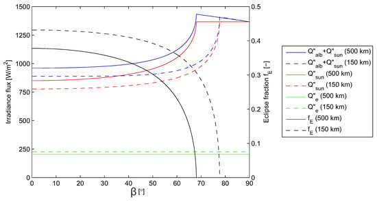
Figure 6.
Irradiance sources and eclipse fraction as function of . The solid lines (—) are valid for the altitude of 500 km and the dashed lines (- -) are for an altitude of 150 km.
For such scenarios of average irradiance, it is also possible to have an idea of the overall satellite’s temperature as a function of . Figure 7 shows the average temperature for different ratios of absorptivity and emissivity (), and two altitudes. In this case, it was assumed a hypothetical geometry whose half of the external surface could absorb the incoming radiation. The average temperature increases with because the eclipse fraction decreases up to the point of and , where it vanishes for altitude 150 km and 500 km, respectively. Beyond these points, the temperature slightly reduces because the albedo load decreases as the satellite moves away from the subsolar point. The temperature increases with altitude for a given because the eclipse fraction is smaller at higher altitudes. This graph also shows that big ratios of increase the temperature since the satellite easily absorbs the radiation while it poorly rejects it. The opposite happens for low values of , where the emission of radiation is more significant than its absorption, resulting in lower temperature values.
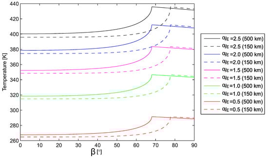
Figure 7.
Average temperature as function of ratio and . The solid lines (—) are valid for the altitude of 500 km and the dashed lines (- -) are for altitude of 150 km.
Figure 8 shows the altitude estimation of TLE1 exposed to four different perturbation models. “No perturbation” neglect any form of perturbation, and its result reproduces a perfect horizontal plot, hard to see because it is behind the model “Drag:-,J2”, this without any drag perturbation and only J2 gravitational perturbation. This last case creates wobbles in the altitude, but the CubeSat does not reduce its altitude permanently. This oscillation is a consequence of short-period variations in the COE, not shown here. When the drag perturbation is introduced, the decay appears. While the orbit’s apogee and perigee are noticeable at the beginning of the simulation, around 196 days after and closer to the reentry, the orbit is almost totally circularized. Finally, with the density model NRLMSISE-00, the simulation shows that the CubeSat’s lifespan is longer than the previous model, taking 305 days to achieve an altitude of 100 km. The results from TLE1 obtained with the atmospheric model NRLMSISE-00 will be used in the next results because it brings better relations of accuracy and computational cost [44,45].
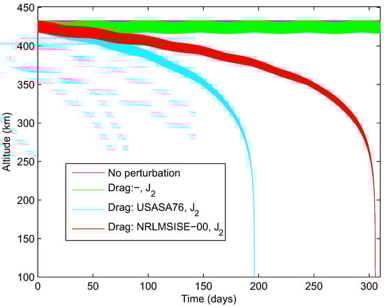
Figure 8.
Altitude evolution for different perturbation models.
The altitude variation of the different perturbation models of this case would have a minor impact in the average irradiance field showed in Figure 6; however, Figure 9 shows that is strongly affected through the lifespan of the CubeSat. The influence of J2 perturbation is evident, essentially because it impacts in the rate of , presented in the formulation of (Equation (39)). On the other hand, the influence of drag is negligible.
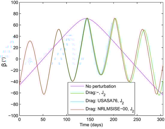
Figure 9.
angle along one year for TLE1 with different perturbation models.
For a particular orbit period with and attitude of Nadir, the total irradiance on each side of a CubeSat is plotted in Figure 10. The gap in the middle of the figure results from the Earth’s eclipse, where only the infrared radiation emitted by the Earth hits the surfaces exposed to it. This attitude has a low irradiance level at surfaces and , a consequence of none solar radiation over them. The opposite sides and have the greatest peaks, while the opposite sides and would also have it if the eclipse did not cut it from .
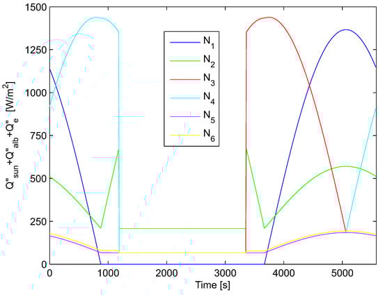
Figure 10.
Total irradiance flux for each side of the CubeSat and average temperature. Orbit with TLE1, , date 10/01/15, 00:00 am, attitude Nadir and perturbation “Drag: NRLMSISE-00, J2”.
The total irradiance flux in the entire CubeSat is shown in Figure 11a,b for the five attitude models discussed earlier, and the extreme conditions of and maximum . Here the importance of is evident, resulting in the maximum eclipse and absence of it for the same initial COE. The case with has the greatest peak and variation of irradiation for a given attitude compared to the case without an eclipse, consequence of albedo radiation through the orbit. In both scenarios of , the maximum amount of irradiation is obtained for the attitude Sun3, where three sides of the CubeSat are equally exposed to the sun constantly, while the minimum is for attitude Sun1, where only one surface sees the sun.
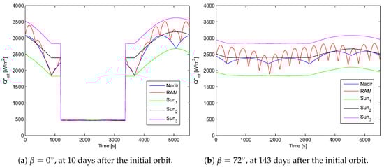
Figure 11.
Total irradiance flux for each attitude, with TLE1 and perturbation “Drag: NLMSISE-00, J2”.
The temperature (T) for the steady-state of a CubeSat 1U with is plotted in Figure 12, for the same conditions of previous Figure 11. In both cases of , the temperature follows the total irradiance trend, as it should be specifically for the case of steady-state. The range of values is between 190 K to 325 K, with the minimum only achieved for the orbit with eclipse.

Figure 12.
Average temperature at steady-state for each attitude, with TLE1 and perturbation “Drag: NLMSISE-00, J2”.
Table 2 summarizes the average temperature values for the entire orbit. Notice that other values are found in Figure 7 for (318 K for both altitudes) and (326 K at the altitude of 150 km and 346 K at 500 km). The reason for such discrepancy relies on the fact that Figure 7 ignores the view factor of surfaces towards the irradiation sources and assumes that half of the satellite’s external surface receives radiation; therefore, it overestimates the targeted area regardless of any attitude model. On the other hand, in Figure 12, the area projection is ruled by the view factors described earlier for a CubeSat geometry and the corresponding attitude model. Nevertheless, the reader should pay attention that the average temperature in Figure 12 ignored the transient term, an essential parameter for the proper prediction of the temperature along an orbit.
Table 2.
Average temperature of the entire orbit for different attitudes and .
In order to validate the model here presented, one must rely on data that are not easily available [59], and when available, maybe from different CubeSat designs [60], with few samples, or even incomplete for reproduction since the output may result from the combination of different conditions found during the operation in orbit. Nevertheless, [61,62] emphasize the importance of extensive simulations before the satellite’s flight operation. Therefore, it is understood that the validation of the models will become more comfortable with the advent of more CubeSat’s launches.
5. Illustrative Application
This section presents the use of the irradiance model proposed here to improve other algorithms for CubeSats used in the literature. Here we focus on sample usages to improve task scheduling algorithms; however, other usages are also subject to improvements. For example, in [63] the authors performed an experimental evaluation of thermoelectric generators (TEGs) for nanosatellites application with orbit’s simulation controlling the temperature on the sides of the TEG. Another example is the experimental and numerical analysis of Electrical Power Systems (EPS) architectures, a critical subsystem in CubeSats [64]. In general, it is understood that the more accurate the orbit and irradiance model is, the more accurate will be the applications that use these models as input data.
The most simple equation to estimate the power generation through photovoltaic solar panels (PV) includes the efficiency term (), the flux of irradiation (), and the area of PV (A):
One additional term can be introduced to account for the natural degradation of PV in the space environment [65], the life degradation ():
So, the power generation considering the degradation will be:
The above equations will be applied in an optimization problem dedicated for CubeSat, with the following parameters: , cm, 60.36 cm (CubeSat 2U), and degradation per year of 2.75%.
Offline Task Scheduling
In [4], the authors formulated the scheduling problem of a Cubesat using mathematical integer programming (IP) to maximize the number of priority tasks to be executed by the satellite, constrained to the amount of power input coming from the solar panels at any moment along the course of an orbit. The authors assume that the maximum power input for each minute along the orbit is known since the scheduling is done on land, previously considering the orbit of the Cubesat of interest. Thus, the more accurate the power estimation, the better the task scheduling. A simplified IP formulation, based on [4], is presented trough Equation (45) and the definitions for the notations are given in Table 3.
Table 3.
Sets, variables and constants.
The formulation objective (45a) maximizes the value of the sum of the priorities of all tasks initiated along an orbit, ensuring that higher priority tasks will have a bigger weight and, consequently, preference in time assignment. The constraint (45b) ensures that the power used by all jobs at any given moment is smaller than the available power at that moment. Constraints (45c), (45d), (45e), (45f) and (45g) force the auxiliary variable to detect the startup of a job by taking the value of 1 only at the unit of time t that a job initiated. Likewise, (45h) and (45i) limit the minimum and the maximum number of starts for a job in an orbit. Equations (45j), (45k) and (45l) ensure the time assigned to each job is withing minimum and maximum CPU execution time required by it. Constraints (45m) and (45n) ensure that each task will be executed only once in a given period.
The cases to be tested in the IP formulation mentioned above are presented in Table 4. To exemplify the impact of the power input model on the task scheduling, and consequently, on the mission quality-of-service, our proposed methodology will be compared with an ideal case, typically assumed in CubeSat projects’ development. This ideal scenario assumes that the engineer does not have a flexible and integrated model to assess the power generation of a 2U CubeSat with PV covering its external surfaces. We start with the premise that the CubeSat will be launched from the ISS. In an ideal and simplified case, the user assumes that in the Beginning-Of-Life (BOL) the orbit is circular, the altitude is 430 km, the inclination is 51.6°, the eclipse is maximum, and the satellite keeps its rotation synchronized with its translation around the Earth, which is equivalent to the attitude Nadir. The user assumes the sun’s irradiation as the energy source for photovoltaic panels’ power generation. We will name this case as . Another condition that the user is also interested in is the performance near the End-of-Life (EOL) of the CubeSat. The only difference from the previous case is that an altitude of 150 km is assumed. This case we will call as . With identical parameters of the last scenario, the user also conducts a third case where he considers that the satellite spends six months in orbit and then includes the PV degradation (Equation (43)) in the estimation of power (Equation (42)). For this case, the name will be .
Table 4.
Scenarios for power scheduling.
On the other hand, with the more realistic methodology proposed in this paper, we will have the following considerations. The CubeSat will align the biggest axis of the satellite with the velocity vector, and the satellite will spin about this axis at the arbitrary rate of four revolutions per orbit to mimic a residual angular speed. This is a scenario achieved with active attitude control and identical to the RAM attitude discussed earlier. The PV will use both direct solar radiation and albedo as input for power generation. The orbit conditions for the BOL’s proposed methodology will be TLE1 and the date of 1 January 2015. Such a scenario will be called . If we are interested in the performance of this same CubeSat 30 days before the CubeSat reentry, we can check Figure 8 and realize it will happen 275 days after the launch. This case will be the . Finally, the last case will use the same information as the previous case, including the panel degradation formulation, with 2.75% of degradation per year. This case will be . All of these scenarios are summarized in Table 4.
Finally, the power input was computed in a minute-by-minute basis for all cases and multiplied by an Electrical Power System (EPS) efficiency factor of 0.85 [23] in order to obtain the energy available to the satellite tasks. In this sense, an offline scheduling algorithm can help the engineer to estimate whether the satellite will be able to handle, for example, the desired amount of payloads. Thus, even subject to input power estimation errors, it can be verified whether tasks would be performed with the desired frequency or whether it would be necessary, for example, to reduce the number of payloads. Considering the scheduling data of the 2U satellite of [66], here shown in Table 5, the scheduling formulation was solved using the Gurobi solver [67] in a PC with Intel(R) Core(TM) i7-8550U 1.8 GHz, 16GB of RAM and Windows 10 64 bits.
Table 5.
2U nanosatellite payloads scheduling data.
The results for and are shown in Figure 13 and Figure 14 for the power usage and the scheduling results, respectively. It can be noticed that the available power is higher at the BOL when the proposed model is considered, and, as a consequence, the number of tasks executed. Figure 15 and Figure 16 present the power usage for EOL and EOL with degradation, respectively. The same result is observed for these two cases, demonstrating a significantly higher calculated power input with the proposed model, sufficient to maintain all of the payloads simultaneously with spare energy—not possible with ideal methodology.
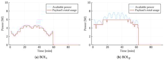
Figure 13.
Power analyses for Beginning-Of-Life (BOL).
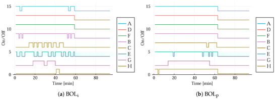
Figure 14.
Scheduling results for BOL.
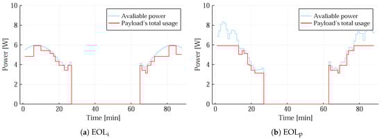
Figure 15.
Power analysis for End-Of-Life (BOL).
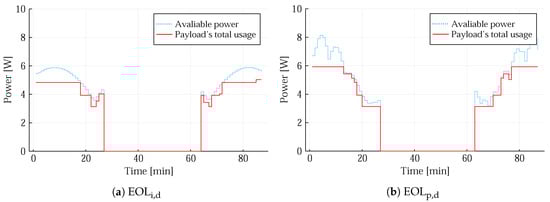
Figure 16.
Power analysis for EOL with degradation.
To show the impact on mission extraction of value, Figure 17 presents the value of the objective function (45a) (the quality of service) obtained for each of the instances along with the computational solving time of the scheduling algorithms. Significant differences can be noticed between the quality of service of the ideal scenarios and the scenarios modeled with the methodology modeled here. Besides, it can be seen that the quality of the service delivered decreases over the life of the satellite, although the lifespan was short, 180 and 275 days for the scenario with degradation in the ideal and proposed cases, respectively.
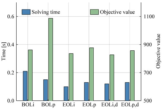
Figure 17.
Scheduling solving time and resulting objective value for each power input scenario.
6. Conclusions
Considering the need for engineers to simulate, understand the satellite’s behavior in orbit, and minimize failures or an inadequate satellite operation, this paper presented a numerical tool to explore typical irradiation scenarios for CubeSat missions combining state-of-the-art models. In this sense, three main models were considered to estimate the irradiation flux over a CubeSat, namely an orbit, an attitude, and a radiation source model, including solar, albedo, and infrared emitted by the Earth.
Results showed that the altitude impacts the average irradiance sources; however, the influence of is more remarkable, especially near before the end of the eclipse. As a consequence of irradiation, the average temperature follows this same tendency, with larger absorptivity over emissivity ratios resulting in hotter scenarios, as expected. A case study for a typical CubeSats’ TLE (two-line element set), different perturbations, and five attitudes were presented to illustrate the tool’s abilities. Results showed that drag was essential to predict the decay of the satellite with atmospheric model NRLMSISE-00. The inclusion of the J2 was essential to obtain the orbit orientation towards the Sun through the satellite’s lifespan, consequently the solar and albedo flux. The attitude models originated different irradiance scenarios for the CubeSat, reinforcing the importance of this parameter for irradiation estimation, for example, the heat transfer and energy harvesting of satellites.
The paper presents a possible application of the tool as an input to a CubeSat offline task-scheduling procedure. The scheduler uses an input power estimation previously calculated by the model, seeking proximity to reality. The results showed that the complete model’s use had considerable differences from the simplified models sometimes used in the literature. Our proposed model resulted in a considerably higher power input than the simplified idealized methodologies, enabling better mission extraction of value and quality-of-service guarantees.
Therefore, from the above results, it is evident that the orbit dynamic’s proper estimation is crucial. It is suggested that future works upgrade the albedo formulation by considering the albedo reflection function of the latitude and longitude instead of a constant and cosine function. Another useful improvement would be an attitude model whose inertia momentum of the CubeSat and its mass distribution become part of calculations and couple this resulting attitude in the perturbation model’s drag coefficient. Future work may relate to the use of the proposed methodology in conjunction with simulation frameworks for real-time scheduling algorithms.
Author Contributions
Conceptualization, E.M.F. and L.O.S.; methodology, E.M.F.; software, E.M.F. and C.A.R.; validation, E.M.F., L.O.S. and C.A.R.; supervision, L.O.S. and V.d.P.N.; writing—original draft preparation, E.M.F., L.O.S. and C.A.R.; writing—review and editing, V.d.P.N., R.G.O., and V.R.Q.L.; funding acquisition, R.G.O., and V.R.Q.L. All authors have read and agreed to the published version of the manuscript.
Funding
This research was partially funded by partially supported by CNPq/Brazil grant number 141196/2019-0 and 141276/2018-5; also by Fundación M. D. Samuel Solórzano Barruso. Proyecto FS/21-2019.
Conflicts of Interest
The authors declare no conflict of interest.
Abbreviations
The following abbreviations are used in this manuscript:
| AU | Astronomical Unit |
| BOL | Begin-of-Life |
| COE | Classical Orbital Element |
| EOL | End-of-Life |
| EPS | Electrical Power system |
| IP | Integer Programming |
| ISS | International Space Station |
| LEO | Low Earth Orbit |
| PV | Photovoltaic solar panel |
| TLE | Two Line Element |
References
- Dida, A.H.; Bekhti, M. Study, modeling and simulation of the electrical characteristic of space satellite solar cells. In Proceedings of the 2017 IEEE 6th International Conference on Renewable Energy Research and Applications (ICRERA), San Diego, CA, USA, 5–8 November 2017; pp. 983–987. [Google Scholar]
- Langer, M.; Bouwmeester, J. Reliability of CubeSats-Statistical Data, Developers’ Beliefs and the Way Forward. In Proceedings of the 2016 30th Annual AIAA/USU Conference on Small Satellites, SSC16-X-2, Logan, UT, USA, 6–11 August 2016; pp. 1–12. [Google Scholar]
- ESA/ESTEC. Product and Quality Assurance Requirements for In-Orbit Demonstration CubeSat Projects. Available online: http://emits.sso.esa.int/emits-doc/ESTEC/AO8352_AD2_IOD_CubeSat_PQA_Reqts_Iss1_Rev1.pdf (accessed on 3 December 2020).
- Rigo, C.A.; Seman, L.O.; Camponogara, E.; Morsch Filho, E.; Bezerra, E.A. Task scheduling for optimal power management and quality-of-service assurance in CubeSats. Acta Astronaut. 2021, 179, 550–560. [Google Scholar] [CrossRef]
- Cho, M.; Hirokazu, M.; Graziani, F. Introduction to lean satellite and ISO standard for lean satellite. In Proceedings of the 2015 7th International Conference on Recent Advances in Space Technologies (RAST), Istanbul, Turkey, 16–19 June 2015; pp. 789–792. [Google Scholar]
- Chin, A.; Coelho, R.; Nugent, R.; Munakata, R.; Puig-Suari, J. CubeSat: The pico-satellite standard for research and education. In Proceedings of the AIAA Space 2008 Conference & Exposition, San Diego, CA, USA, 9–11 September 2008. [Google Scholar] [CrossRef]
- Oh, H.; Park, T. Experimental feasibility study of concentrating photovoltaic power system for cubesat applications. IEEE Trans. Aerosp. Electron. Syst. 2015, 51, 1942–1949. [Google Scholar] [CrossRef]
- Dehbonei, H.; Lee, S.R.; Nehrir, H. Direct Energy Transfer for High Efficiency Photovoltaic Energy Systems Part I: Concepts and Hypothesis. IEEE Trans. Aerosp. Electron. Syst. 2009, 45, 31–45. [Google Scholar] [CrossRef]
- Chin, K.B.; Brandon, E.J.; Bugga, R.V.; Smart, M.C.; Jones, S.C.; Krause, F.C.; West, W.C.; Bolotin, G.G. Energy Storage Technologies for Small Satellite Applications. Proc. IEEE 2018, 106, 419–428. [Google Scholar] [CrossRef]
- Qiao, L.; Rizos, C.; Dempster, A.G. Analysis and comparison of CubeSat lifetime. In Proceedings of the 12th Australian Space Conference, Melbourne, Australia, 24–26 September 2012; pp. 249–260. [Google Scholar]
- Knap, V.; Vestergaard, L.K.; Stroe, D.I. A Review of Battery Technology in CubeSats and Small Satellite Solutions. Energies 2020, 13, 4097. [Google Scholar] [CrossRef]
- Aung, H.; Soon, J.J.; Goh, S.T.; Lew, J.M.; Low, K. Battery Management System With State-of-Charge and Opportunistic State-of-Health for a Miniaturized Satellite. IEEE Trans. Aerosp. Electron. Syst. 2020, 56, 2978–2989. [Google Scholar] [CrossRef]
- Filho, E.M.; de Paulo Nicolau, V.; de Paiva, K.V.; Possamai, T.S. A comprehensive attitude formulation with spin for numerical model of irradiance for CubeSats and Picosats. Appl. Therm. Eng. 2020, 168, 114859. [Google Scholar] [CrossRef]
- Corpino, S.; Caldera, M.; Nichele, F.; Masoero, M.; Viola, N. Thermal design and analysis of a nanosatellite in low earth orbit. Acta Astronaut. 2015, 115, 247–261. [Google Scholar] [CrossRef]
- Bonnici, M.; Mollicone, P.; Fenech, M.; Azzopardi, M.A. Analytical and numerical models for thermal related design of a new pico-satellite. Appl. Therm. Eng. 2019, 159, 113908. [Google Scholar] [CrossRef]
- Claricoats, J.; Dakka, S.M. Design of Power, Propulsion, and Thermal Sub-Systems for a 3U CubeSat Measuring Earth’s Radiation Imbalance. Aerospace 2018, 5, 63. [Google Scholar] [CrossRef]
- Kovács, R.; Józsa, V. Thermal analysis of the SMOG-1 PocketQube satellite. Appl. Therm. Eng. 2018, 139, 506–513. [Google Scholar] [CrossRef]
- Hawkins, E.M.; Kanapskyte, A.; Maria, S.R.S. Developing Technologies for Biological Experiments in Deep Space. Proceedings 2020, 60, 28. [Google Scholar] [CrossRef]
- Diaz-Aguado, M.F.; Ghassemieh, S.; Van Outryve, C.; Beasley, C.; Schooley, A. Small Class-D spacecraft thermal design, test and analysis—PharmaSat biological experiment. In Proceedings of the 2009 IEEE Aerospace Conference, Big Sky, MT, USA, 7–14 March 2009; pp. 1–9. [Google Scholar] [CrossRef]
- Ibrahim, S.A.; Yamaguchi, E. Comparison of Solar Radiation Torque and Power Generation of Deployable Solar Panel Configurations on Nanosatellites. Aerospace 2019, 6, 50. [Google Scholar] [CrossRef]
- Piedra, S.; Torres, M.; Ledesma, S. Thermal Numerical Analysis of the Primary Composite Structure of a CubeSat. Aerospace 2019, 6, 97. [Google Scholar] [CrossRef]
- Scheeres, D.J. Satellite dynamics about small bodies: Averaged solar radiation pressure effects. J. Astronaut. Sci. 1999, 47, 25–46. [Google Scholar] [CrossRef]
- Marcelino, G.M.; Vega-Martinez, S.; Seman, L.O.; Kessler Slongo, L.; Bezerra, E.A. A Critical Embedded System Challenge: The FloripaSat-1 Mission. IEEE Lat. Am. Trans. 2020, 18, 249–256. [Google Scholar] [CrossRef]
- Slongo, L.K.; Martínez, S.V.; Eiterer, B.V.; Pereira, T.G.; Bezerra, E.A.; Paiva, K.V. Energy-driven scheduling algorithm for nanosatellite energy harvesting maximization. Acta Astronaut. 2018, 147, 141–151. [Google Scholar] [CrossRef]
- Corpino, S.; Stesina, F. Verification of a CubeSat via hardware-in-the-loop simulation. IEEE Trans. Aerosp. Electron. Syst. 2014, 50, 2807–2818. [Google Scholar] [CrossRef]
- Kiesbye, J.; Messmann, D.; Preisinger, M.; Reina, G.; Nagy, D.; Schummer, F.; Mostad, M.; Kale, T.; Langer, M. Hardware-In-The-Loop and Software-In-The-Loop Testing of the MOVE-II CubeSat. Aerospace 2019, 6, 130. [Google Scholar] [CrossRef]
- Raif, M.; Walter, U.; Bouwmeester, J. Dynamic system simulation of small satellite projects. Acta Astronaut. 2010, 67, 1138–1156. [Google Scholar] [CrossRef]
- Gilmore, D.; Donabedian, M. Spacecraft Thermal Control Handbook: Fundamental Technologies; Spacecraft Thermal Control Handbook; Aerospace Press: El Segundo, CA, USA, 2002. [Google Scholar]
- Berg, L.K.; Long, C.N.; Kassianov, E.I.; Chand, D.; Tai, S.L.; Yang, Z.; Riihimaki, L.D.; Biraud, S.C.; Tagestad, J.; Matthews, A.; et al. Fine-Scale Variability of Observed and Simulated Surface Albedo Over the Southern Great Plains. J. Geophys. Res. Atmos. 2020, 125, e2019JD030559. [Google Scholar] [CrossRef]
- Cui, Y.; Mitomi, Y.; Takamura, T. An empirical anisotropy correction model for estimating land surface albedo for radiation budget studies. Remote Sens. Environ. 2009, 113, 24–39. [Google Scholar] [CrossRef]
- NASA. Earth Albedo and Emitted Radiation; NASA SP-8067; NASA: Washington, DC, USA, 1971.
- Rodriguez-Solano, C.J.; Hugentobler, U.; Steigenberger, P. Impact of Albedo Radiation on GPS Satellites. In Geodesy for Planet Earth; Kenyon, S., Pacino, M.C., Marti, U., Eds.; Springer: Berlin/Heidelberg, Germany, 2012; pp. 113–119. [Google Scholar]
- Román, M.O.; Schaaf, C.B.; Lewis, P.; Gao, F.; Anderson, G.P.; Privette, J.L.; Strahler, A.H.; Woodcock, C.E.; Barnsley, M. Assessing the coupling between surface albedo derived from MODIS and the fraction of diffuse skylight over spatially-characterized landscapes. Remote Sens. Environ. 2010, 114, 738–760. [Google Scholar] [CrossRef]
- Goode, P.R.; Qiu, J.; Yurchyshyn, V.; Hickey, J.; Chu, M.C.; Kolbe, E.; Brown, C.T.; Koonin, S.E. Earthshine observations of the Earth’s reflectance. Geophys. Res. Lett. 2001, 28, 1671–1674. [Google Scholar] [CrossRef]
- Brennan, M.; Abramase, A.; Andrews, R.; Pearce, J. Effects of spectral albedo on solar photovoltaic devices. Sol. Energy Mater. Sol. Cells 2014, 124, 111–116. [Google Scholar] [CrossRef]
- Li, S.; Wang, Y.; Zhang, H.E.A. Thermal Analysis and Validation of GF-4 Remote Sensing Camera. J. Therm. Sci. 2020, 29, 992–1000. [Google Scholar] [CrossRef]
- Zheng, C.; Qi, J.; Song, J.; Cheng, L. Numerical investigation on the thermal performance of Alpha Magnetic Spectrometer main radiators under the operation of International Space Station. Numer. Heat Transf. Part A Appl. 2020, 77, 538–558. [Google Scholar] [CrossRef]
- Reyes, L.A.; Cabriales-Gómez, R.; Chávez, C.E.; Bermúdez-Reyes, B.; López-Botello, O.; Zambrano-Robledo, P. Thermal modeling of CIIIASat nanosatellite: A tool for thermal barrier coating selection. Appl. Therm. Eng. 2020, 166, 114651. [Google Scholar] [CrossRef]
- Haneveer, M.R. Orbital Lifetime Predictions: An assessment of Model-Based Ballistic Coefficient Estimations and Adjustment for Temporal Drag Coefficient Variations. Master’s Thesis, Delft University of Technology, Delft, The Netherlands, 2017. [Google Scholar]
- Curtis, H.D. Orbital Mechanics for Engineering Students, 3rd ed.; Butterworth-Heinemann: Boston, MA, USA, 2014; p. 751. [Google Scholar] [CrossRef]
- Capderou, M. Handbook of Satellite Orbits: From Kepler to GPS; Springer International Publishing: Cham, Switzerland, 2014. [Google Scholar]
- McClain, W.; Vallado, D. Fundamentals of Astrodynamics and Applications; Space Technology Library; Springer: Dordrecht, The Netherlands, 2001. [Google Scholar]
- Atallah, A.M.I. A Implementation and Verification of a High-Precision Orbit Propagator. Master’s Thesis, Cairo University, Cairo, Egypt, 2018. [Google Scholar]
- Vallado, D.; Finkleman, D. A Critical Assessment of Satellite Drag and Atmospheric Density Modeling. Acta Astronaut. 2014, 95, 141–165. [Google Scholar] [CrossRef]
- Picone, J.M.; Hedin, A.E.; Drob, D.P.; Aikin, A.C. NRLMSISE-00 empirical model of the atmosphere: Statistical comparisons and scientific issues. J. Geophys. Res. Space Phys. 2002, 107, 15–16. [Google Scholar] [CrossRef]
- Park, D.; Miyata, K.; Nagano, H. Thermal design and validation of radiation detector for the ChubuSat-2 micro-satellite with high-thermal-conductive graphite sheets. Acta Astronaut. 2017, 136, 387–394. [Google Scholar] [CrossRef]
- Mason, J.P.; Lamprecht, B.; Woods, T.N.; Downs, C. CubeSat On-Orbit Temperature Comparison to Thermal-Balance-Tuned-Model Predictions. J. Thermophys. Heat Transf. 2018, 32, 237–255. [Google Scholar] [CrossRef]
- Lee, S.; Hong, Z.; Peng, K.; Leu, L. Analysis the Unsteady-State Temperature Distribution of Micro-Satellite Under Stabilization Effects. In Microsatellites as Research Tools; COSPAR Colloquia Series; Hsiao, F.B., Ed.; Pergamon: Kaohsiung, Taiwan, 1999; Volume 10, pp. 324–332. [Google Scholar] [CrossRef]
- Farhani, F.; Anvari, A. Effects of Some Parameters on Thermal Control of a LEO Satellite. J. Space Sci. Technol. 2014, 7, 13–24. [Google Scholar]
- Roldugin, D.; Testani, P. Spin-stabilized satellite magnetic attitude control scheme without initial detumbling. Acta Astronaut. 2014, 94, 446–454. [Google Scholar] [CrossRef]
- Xing, Y.; Cao, X.; Zhang, S.; Guo, H.; Wang, F. Relative position and attitude estimation for satellite formation with coupled translational and rotational dynamics. Acta Astronaut. 2010, 67, 455–467. [Google Scholar] [CrossRef]
- Auret, J.; Steyn, W. Design of an aerodynamic attitude control system for a CubeSat. In Proceedings of the 62nd International Astronautical Congress 2011 (IAC 2011) Cape Town, South Africa, 3–7 October 2011; Volume 11, pp. 9009–9017. [Google Scholar]
- Bate, R.; Mueller, D.; White, J. Fundamentals of Astrodynamics; Dover Books on Aeronautical Engineering Series; Dover Publications: New Yourk, USA, 1971. [Google Scholar]
- Schaub, H.; Junkins, J. Analytical Mechanics of Space Systems; AIAA Education Series; American Institute of Aeronautics and Astronautics, Incorporated: Reston, VA, USA, 2014. [Google Scholar]
- Xiao, B.; Huo, M.; Yang, X.; Zhang, Y. Fault-Tolerant Attitude Stabilization for Satellites Without Rate Sensor. IEEE Trans. Ind. Electron. 2015, 62, 7191–7202. [Google Scholar] [CrossRef]
- Pham, M.D.; Low, K.S.; Goh, S.T.; Chen, S. Gain-scheduled extended kalman filter for nanosatellite attitude determination system. IEEE Trans. Aerosp. Electron. Syst. 2015, 51, 1017–1028. [Google Scholar] [CrossRef]
- Richmond, J. Adaptive Thermal Modeling Architecture For Small Satellite Applications. Ph.D. Thesis, Massachusetts Institute of Technology, Department of Aeronautics and Astronautics, Cambridge, MA, USA, 2010. [Google Scholar]
- Mahooti, M. NRLMSISE00 Atmospheric Density Model. MATLAB Central File Exchange. Available online: https://www.mathworks.com/matlabcentral/fileexchange/54673-nrlmsise00-atmospheric-density-model (accessed on 10 October 2020).
- Yamagiwa, Y.; Fujii, T.; Nakashima, K.; Oshimori, H.; Okino, T.; Komua, S.; Arita, S.; Nohmi, M.; Ishikawa, Y. Space experimental results of STARS-C CubeSat to verify tether deployment in orbit. Acta Astronaut. 2020, 177, 759–770. [Google Scholar] [CrossRef]
- Kim, O.J.; Shim, H.; Yu, S.; Bae, Y.; Kee, C.; Kim, H.; Lee, J.; Han, J.; Han, S.; Choi, Y. In-Orbit Results and Attitude Analysis of the SNUGLITE Cube-Satellite. Appl. Sci. 2020, 10, 1507. [Google Scholar] [CrossRef]
- Nies, G.; Stenger, M.; Krčál, J.; Hermanns, H.; Bisgaard, M.; Gerhardt, D.; Haverkort, B.; Jongerden, M.; Larsen, K.G.; Wognsen, E.R. Mastering operational limitations of LEO satellites—The GomX-3 approach. Acta Astronaut. 2018, 151, 726–735. [Google Scholar] [CrossRef]
- Tejumola, T.R.; Zarate Segura, G.W.; Kim, S.; Khan, A.; Cho, M. Validation of double Langmuir probe in-orbit performance onboard a nano-satellite. Acta Astronaut. 2018, 144, 388–396. [Google Scholar] [CrossRef]
- Ostrufka, A.; Filho, E.; Borba, A.; Spengler, A.; Possamai, T.; Paiva, K. Experimental evaluation of thermoelectric generators for nanosatellites application. Acta Astronaut. 2019, 162, 32–40. [Google Scholar] [CrossRef]
- Kessler Slongo, L.; Vega Martínez, S.; Vale Barbosa Eiterer, B.; Augusto Bezerra, E. Nanosatellite electrical power system architectures: Models, simulations, and tests. Int. J. Circuit Theory Appl. 2020, 48, 2153–2189. [Google Scholar] [CrossRef]
- Wertz, J.; Larson, W. Space Mission Analysis and Design; Space Technology Library; Springer: Dordrecht, The Netherlands, 1999. [Google Scholar]
- Rigo, C.A.; Seman, L.O.; Camponogara, E.; Morsch Filho, E.; Slongo, L.K.; Bezerra, E.A. Mission plan optimization strategy to improve nanosatellite energy utilization and tasks QoS capabilities. In Proceedings of the IV IAA Latin American Cubesat Workshop (IAA-LACW’2020), Rome, Italy, 28–31 January 2020. [Google Scholar]
- Gurobi Optimization, LCC. Gurobi Optimizer Reference Manual. Available online: https://www.gurobi.com/wp-content/plugins/hd_documentations/documentation/9.1/refman.pdf (accessed on 10 September 2020).
Publisher’s Note: MDPI stays neutral with regard to jurisdictional claims in published maps and institutional affiliations. |
© 2020 by the authors. Licensee MDPI, Basel, Switzerland. This article is an open access article distributed under the terms and conditions of the Creative Commons Attribution (CC BY) license (http://creativecommons.org/licenses/by/4.0/).