Abstract
Harmonic overvoltage in electric railway traction networks can pose a serious threat to the safe and stable operation of the traction power supply system (TPSS). Existing studies aim at improving the control damping of grid-connected converters, neglecting the impedance frequency characteristics (IFCs) of the actual TPSS. The applicable frequency range of these studies is relatively low, usually no more than half of the switching frequency, and there is a large gap with the actual traction network harmonic overvoltage frequency range of 750 Hz–3750 Hz. In this paper, first, the IFCs of the actual TPSS in the wide frequency range of 150 Hz–5000 Hz are obtained through field tests, and the resonant frequency distribution characteristics of TPSS are analyzed. After that, the aliasing effect of the sampling process and the sideband effect of the modulation process of the digital control of the grid-connected converter are considered. Based on the relative relationships among the inherent resonant frequency of the TPSS, sampling frequency and switching frequency, an impedance matching analysis method is proposed for the wide frequency range of the vehicle–grid coupling system. By this method, the sampling frequency and switching frequency can be decoupled, and the harmonic overvoltage of traction network in the frequency range of two times switching frequency and above can be directly estimated. Finally, the method proposed in this paper is validated by the comparative simulation analysis of seven different cases.
1. Introduction
Since alternating current-direct current-alternating current (AC-DC-AC) Electric Multiple Units (EMUs) and electric locomotives have been adopted widely in China, the traction power supply system (TPSS) and electric locomotives’ electrical matching instability caused by high-order harmonic overvoltage traction network problems occur from time to time. Harmonic overvoltage of traction networks can cause the substation feeder to trip. In severe cases, it will cause damage to the high-voltage equipment of the catenary, the on-board high-voltage equipment, and the electrical equipment in the substation. In addition, it can even result in the disruption of the locomotive operation [1]. A widely applied method is that the harmonic overvoltage problem of traction networks is mostly regarded as a harmonic instability problem of the vehicle–grid coupling control system. The method utilizes Re {Zin(jω)} > 0 as stability criterion, where Re {Zin(jω)} > 0 denotes the real part of input impedance of grid-connected converters port. When Zin(jω) does not satisfy the condition that the real part is greater than 0 at a certain frequency, the risk of harmonic instability is considered to exist [2,3,4,5,6]. The European Norm EN 50388, which is enforced by railway administrations in several countries, requires all new elements added to the system checked for compatibility [7]. The standard also specifies that harmonic overvoltage is classified into three main categories: overvoltage caused by system instability, harmonics and other phenomena. However, the standard only requires that in a 25,000 V, 50 Hz network, the peak voltage is always below 50,000 V, which is a lax standard with regard to harmonics. There are two deficiencies in the method that the harmonic overvoltage problem is completely regarded as an equivalent control stability analysis of the grid-connected converter, which makes it difficult to solve practical cases.
The impedance frequency characteristics (IFCs) of the TPSS are deliberately simplified. In the existing literatures, input impedance of traction network is usually represented by a parallel LC circuit. This simple circuit can introduce a parallel resonance. However, the IFCs of the actual TPSS may exhibit multiple parallel resonances, and the resonant frequency is affected by power supply mode, the length of railway, location of the locomotive and other factors. This implies a wide range of resonance frequencies. The discrepancy between the simplified circuit model in a laboratory setting and actual system requires more detailed consideration when analyzing real problems with existing methods. Researchers reckoned that their proposed method may become invalid if there are two resonances on a TPSS with an approximately symmetrical distribution of Nyquist frequency [8]. The current research on this issue is still insufficient, mainly because of the lack of field test data and effective techniques that can test the IFCs of a 25 kV electric railway over a wide frequency range.
The applicable frequency range of the existing research is lower than the switching frequency. Although the influence of complex factors, such as time delay and LCL filters, is taken into consideration, most of the current research has focused on the relatively low frequency range, that is, below the Nyquist sampling frequency or half of the switching frequency. These studies do not apply to real on-board grid-connected converters switching frequency of only a few hundred hertz, while harmonic overvoltage frequency can reach thousands of hertz (several times the switching frequency). Though the published papers [8,9,10] attempt to broaden the frequency range applicable to the study by considering the aliasing effect of the converter-controlled sampling processes, these studies are mostly limited by the premise assumptions fsam = fsw or fsam = 2 fsw. The pulse-width modulation (PWM) element can be simplified into a proportional element. However, in practice, due to the multiplexed or modular cascade structure of the grid-connected converter, the multiplicative relationship between fsam and fsw can be 0.5-fold, 1-fold, 2-fold, 4-fold or even any frequency multiplicity [11]. Therefore, the current study is limited in terms of its applicable frequency range.
In the simulation or experiment of previous studies, the switching frequency of the converter or the sampling frequency of the controller is much higher than the resonant frequency of the impedance network. In most studies, the resonant frequency of the impedance network is less than half of the sampling frequency and switching frequency (see Table 1). That is, the sampling frequency and switching frequency are much larger than the Nyquist frequency. In addition, in almost all previous studies, the ratio of the switching frequency of the converter to the sampling frequency of the controller is fixed at 2:1, 1:1 or 1:2 and there is a lack of research on other ratios. Furthermore, the switching frequency of the converter often ranges from 2 kHz to higher than 10 kHz in previous studies, while in actual railway systems, the switching frequency of the train converter is usually in the range of 250–1250 Hz. There is a large difference between the two frequency ranges. In our earlier research, the resonance frequency of TPSS under different operation conditions is distributed in a wide frequency range of hundreds to more than 3000 Hz.

Table 1.
Comparison among different frequencies.
All in all, it can be deduced that, in reality, the resonant frequency of the traction network may be: 1. above the sampling frequency of the train converter; 2. below the sampling frequency and within the range of Nyquist frequency (0—half of the sampling frequency); 3. below the sampling frequency but between the Nyquist frequency and the sampling frequency.
Our work is more effective than previous research. This paper investigates the mechanism of resonant overvoltage in a wider frequency range, that is, all of the above three cases. In addition, this paper also considers more combinations of the ratio of the sampling frequency (fsam) to the switching frequency (fsw), which can be categorized into four situations: (a.) 2 fsam ≤ fsw; (b.) fsw ≤ fsam < 2 fsw; (c.) 2 fsw ≤ fsam < 4 fsw; (d.) 4 fsw ≤ fsam. Taking the above mentioned three cases and four situations into account, this paper provides a wider vision to the TPSS resonant overvoltage problem.
To address the above research deficiencies, this paper mainly focuses on harmonic overvoltage of the traction network with a wide frequency range. First of all, this paper presents the results of the impedance frequency characteristics test and analyzes the inherent resonant frequency distribution characteristics of the traction network. Moreover, the aliasing effect of the converter control processes and the PWM sideband effect are taken into consideration in this paper. The relative magnitude relationship of the traction network impedance resonant frequency, sampling frequency and PWM switching frequency is considered. The obtained model is suitable for any multiple relationship between fsw and fsam, and can suppress harmonic overvoltage of the traction network by changing fsw and fsam. This paper presents the link between the steady-state waveform of traction network harmonic overvoltage and the control stability of the vehicle–grid coupling system, and proposes a formula for the harmonic overvoltage of the traction network, which makes a comprehensive description of the harmonic overvoltage of the traction network of the network coupling system.
where represents the harmonic overvoltage, is the impedance matrix of vehicle–grid coupling system, is the control coupling coefficient matrix, is the harmonic source matrix. Equation (1) has the form and dimension of Ohm’s law, which can take all the variables and parameters of the vehicle–grid coupling system into account. Equation (1) will be elaborated on below.
2. Vehicle–Grid Coupling System
Vehicle–Grid Coupling System Model
In Figure 1, it is shown that the electrified railway vehicle–grid coupling system is mainly composed of TPSS and on-board converter.
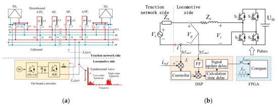
Figure 1.
Model of the vehicle–grid coupling system. (a) Actual railways; (b) the converter model.
The TPSS is made up of multiple subsystems: substation (SS), auto-transformer post (ATP), section post (SP), rail, over contact line (OLC), positive feeder (PF), and multi-conductor transmission line traction network with complex structure and parameters. The model of the on-board converter is shown in Figure 1b. The design of the converter digital control system on control logic includes digital signal processor (DSP) and field-programmable gate array (FPGA). The control algorithm is implemented on DSP. FPGA is used to execute modulation algorithms. The actual power supply operation mode is AT/double traction/parallel lines/overhead contact line–classic–hanging. The railroad section researched was not covered by a tunnel.
The Root Mean Square (RMS) and instantaneous value waveforms of voltage, before and after the tripping of the T-bus of a traction substation, are depicted in Figure 2. The measuring data of the traction substation are from one case of [1]. The general procedure for evaluating harmonic overvoltage based on measured waveforms is: Fourier analysis is performed on the measured instantaneous waveforms to obtain the magnitude and frequency of each order harmonics of traction network voltage, and then the frequency of the harmonic component with the largest amplitude is taken as the traction network voltage resonant frequency [1,12,13]. According to this procedure, the resonant frequency of the traction network voltage shown in Figure 2 is 950 Hz. In order to distinguish the terms’ resonant frequency in the control system from the inherent resonant frequency of the TPSS, this paper refers to the frequency of the harmonic component with the largest amplitude in the traction network voltage as the traction network resonant overvoltage frequency fhv.
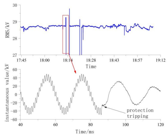
Figure 2.
Harmonic overvoltage waveforms of the traction network in actual railways.
3. IFCs of TPSSs
The authors’ previous research has proposed a harmonic impedance testing method based on a harmonic generator (HG) constructed with cascaded H-bridge converters, which can directly measure the input harmonic impedance of the 25 kV electric railway traction network port in the range of 5000 Hz. The test method and implementation process have been presented in detail in the literature [14,15]. Operation of the telecontrol switches 1–28 in Figure 1a to switch the different power supply modes, during the test, is shown in Table 2. Here, we inject the harmonic current with a harmonic source and obtain harmonic impedance by the method of harmonic voltage and current test [1]. Eventually, the IFCs of the TPSSs are obtained at SP1 under different operating modes. The test results are depicted in Figure 3.
Table 2.
Switch operation table during the impedance frequency characteristic (IFC) tests.
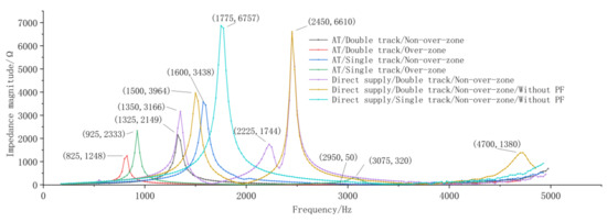
Figure 3.
Impedance frequency characteristics of the actual railway by field tests.
The test results shown in Figure 3 indicate that the inherent resonant frequency of the TPSS itself is affected by factors such as length of the traction network (over-zone vs. non-over-zone test), auto-transformer (AT vs. direct supply test), line type (single track vs. double track railway test), and the structure of the traction network (with or without a PF comparison test), which are subject to complex variations. In addition, the existence of more than two resonances for the over-zone feeding with a long power supply section provides measured data and supporting evidence for the potential problems identified in [8]. The above results indicate that the complex IFCs of the actual traction network and its own inherent resonance bring great challenges to the analysis of the vehicle–grid coupling system and the control design and parameter setting of the grid-connected converter.
4. Control Modeling of Converters
4.1. Sampling Process and Aliasing Effect
Consider the sampling process of voltage Vg, and current i, as shown in the Figure 4. When the original signal frequency X(jω) is less than the Nyquist sampling frequency, the sampling output R(jω) will be attached to generate a high-frequency interference signal. If the frequency distance between the signals is large, the low-pass filter can be used to recover the original signal from the sampled signal, that is V(jω). If the frequency of X(jω) is greater than or equal to the Nyquist sampling frequency, the original signal will additionally generate a low-frequency sampling signal. Low-pass filter will not be used to recover the original signal from the sampled signal. In Figure 4, it leads to the effect of spectrum aliasing.
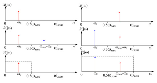
Figure 4.
Diagram of the aliasing effect.
Considering the effect of the aliasing effect, there are multiple frequency signals in the sampling element at the same time, and signals of various frequencies couple each other. The sampling element can be equivalent to a multi-input multi-output system. The relationship of the input and output system can be described as Equation (2) by matrix. Assuming that the input signal is composed of n frequency components, the output signal will also be composed of n components.
The elements on the main diagonal in (2) are the self-coupling conductivity coefficients, which characterize the input–output relationship of the same frequency signal. The elements on the non-diagonal are the mutual coupling conductivity coefficients, which characterize the input–output relationship of signals of different frequencies.
As shown in Figure 5, in order to obtain the coefficients of A = (aij)n×n by the superposition theorem, let the input signal have only one non-zero element at a time, implying:
where . Take the solution of the conduction coefficients of the first component as an example. As shown in Figure 5, at first, set the amplitude of frequency ωξ of the input signal as 1, and the other components are 0, that is, δ(ω − ωξ). According to the signal equation xp(t) affected after the impulse train and the transfer function of the zero-order holder (ZOH), the amplitude and phase angle curves of each component of the output signal r(t) can be depicted in Figure 5 | r(ω) | and ∠ r(ω), respectively. According to the component represented by the red curves in Figure 5, the self-coupling conductivity coefficient a11, as well as the mutual coupling conductivity coefficients a12, a13, etc., can be obtained. Therefore, the first column element of the conduction matrix in (2) can be obtained.
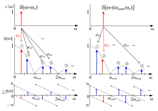
Figure 5.
Derivation of the sampling transfer function at multiple frequencies.
Repeat the above steps until all the elements of the entire matrix are found. It can be written as (4):
where is defined as the transfer function of ZOH.
4.2. Modulation Process and Aliasing Effect
4.2.1. Natural Sampling PWM (NSPWM)
According to the analytical expression [16,18] for the output voltage of a single H-bridge converter NSPWM, the frequency spectrum of the bridge port output voltage varies as the frequency of the modulation waveform gradually increases, and its trajectory is depicted in Figure 6, where the y-axis represents the frequency of the modulation waveform signal and the x–axis represents the frequency spectrum of uc(t). Taking Figure 6 as an example, make tangent 1 parallel to the x–axis at y = 2250 Hz. The tangent plane and trajectory intersect at two points. The value of the x–axis corresponding to the intersection point represents the frequency of the main component of the output voltage. As shown in Figure 6, the pair of natural numbers (m,k) indicates the kth harmonic component of the mth group of sideband harmonics. The baseband trace in Figure 6 represents the component change of the uc(t) at the same frequency as the modulation waveform and is the most dominant component of the PWM modulation process.
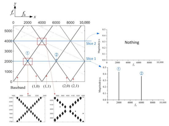
Figure 6.
Locus of the spectral distribution (fs = 2000 Hz, dr = 0.25).
Through the analysis in Figure 6, it can be found that the NSPWM input and output segments are also similar to the sampling process with the aliasing effect. If the frequency of the input modulation wave signal is less than the switching frequency, the output signal will additionally generate a high-frequency interference signal, then the input modulation wave signal can be recovered with a low-pass filter. On the contrary, if the frequency of the input modulation wave signal is greater than the switching frequency, the output signal will additionally produce low-frequency interference. The frequency of the uppermost low-frequency interference component is ωσ − ωο, and the input modulation wave signal cannot be fully recovered by the low-pass filter, as shown in Figure 7. The above NSPWM process can be intuitively understood from the perspective of signal transmission, compared with the switching frequency, the low-frequency original signal will produce additional high-frequency interference, and the high-frequency original signal will produce additional low-frequency interference.
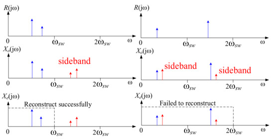
Figure 7.
Diagram of the natural sampling pulse-width modulation (NSPWM) sideband effect.
According to the above analysis, the relationship between the input and output signal of the NSPWM segment can be approximated by (5). represents the relationship between the kth harmonic component of the mth group of sideband harmonics in the output voltage spectrum and the modulation waveform signal. In order to simplify the analysis, only the main 0th and 1st sideband harmonics are considered in Equation (5).
4.2.2. Regular Sampling PWM (RSPWM)
In the method of NSPWM, sinusoidal modulation wave and triangular carrier are compared in real time. Their intersection points are defined by the transcendental equation, which is complicated to solve. In order to facilitate the application in digital control system, the modulation wave is usually sampled and kept constant for a certain period of time; this modulation method is called RSPWM, which can be equated with a sampling segment in series with NSPWM segment. As shown in Figure 8, a simulation is built in the software PSCAD to test the RSPWM input/output signal description function, set fsam = fsw = 2000 Hz, and the cutoff frequency is 5500 Hz.
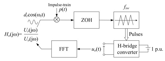
Figure 8.
Test about the signal input–output relation of regular sampling (RSPWM).
Figure 9 shows the results of the test. Spikes within the switching frequency range are due to the aliasing effect of the sampling process. Above the switching frequency range, the aliasing effect and the sideband effect are combined. Figure 9 also shows that the existing research mostly treats the modulation segment as a ZOH segment [9,17], which only performs well in the low-frequency range. However, there are large errors in the high-frequency range.
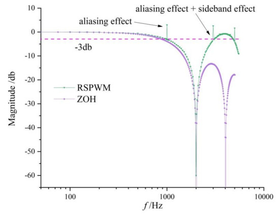
Figure 9.
Amplitude cure of RSPWM in a wide frequency.
5. Harmonic Overvoltage Analysis of Traction Network in a Wide Frequency Range
5.1. Relative Relationship among TPSS Subsection Inherent Resonant Frequency, Sampling Frequency and Switching Frequency
The relative relationship among the inherent resonant frequency (IRF), sampling frequency and switching frequency of the TPSS is shown in Figure 10. As presented in the existing research [11], the switching frequency and sampling frequency can take different ratios. Moreover, inherent resonant frequency of the actual TPSSs is distributed over a wide frequency range, there are different ways of combining the relative value of the three frequency types. According to the analysis in Section 4.1 and Section 4.2, the low-pass filter can be used to recover the original signal at half of fsam and fsw. Therefore, when the IRF of the TPSSs exists in the range of 0.5 fsam ∩ fsw, the low-frequency single-component model can be used for analysis. When IRF2 ε (0.5 fsam, fsw), the aliasing effect of sampling should be considered. When IRF3 ε (fsw,∞), the aliasing effect of sampling and sideband effect should be considered simultaneously. By decomposing the relative relationship of IRF, fsam and fsw, the frequency range of harmonic overvoltage in the traction network can be greatly expanded for research.
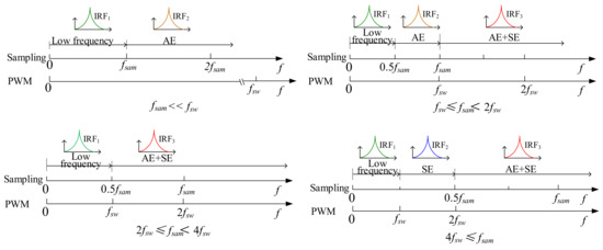
Figure 10.
Relative relations among the IRF, sampling frequency, and switching frequency.
Figure 11 shows a block diagram of a wide frequency range control system considering sampling aliasing effects and modulation sideband effects, where Hcv(s) represents the capacitor voltage controller, Hci(s) represents the current loop controller, Hsam(s) represents the transfer function of the sampling segment, Hffv(s) represents the transfer function of the network voltage feed-forward shown in (4), Gd (s) represents the total delay of the system, Hpwm(s) represents the transfer function of the NSPWM segment shown in (5), Hfbi(s) represents correcting the transfer function of the current sampling sensor.
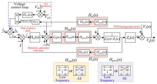
Figure 11.
Control block diagram of the vehicle–grid coupling system at wide frequencies.
5.2. Low-Frequency Range Analysis
In the range of low frequency, the system closed-loop transfer function matrix Hc(s) shown in Figure 11 can be described as:
where Yg is the input admittance of the converter port, Gref is the current control equivalent gain, Yh is the equivalent admittance of voltage fluctuation. According to (6), these three parameters can be measured by small signal frequency scanning for amplitude frequency and phase frequency curves.
Yg, Gref, Yh can be described as:
The traction network voltage Vhv of the vehicle–grid coupling system can be obtained by (6), which can be described as (9):
where Hc11, Hc12, Hc13 are the elements in the corresponding position in Hc(s). The harmonic overvoltage of the traction network can be described as (1).
In (1), it is illustrated that the value of harmonic voltage is closely related to the harmonic impedance matrix Zhv, harmonic gain matrix Hhv, and harmonic noise Ihv: (1) When gets the maximum value at a certain frequency, it means (represents) that this frequency is the resonant frequency of Hhv. In this case, the control of vehicle–grid coupling system will be unstable. With the excitation of limited harmonics, a harmonic overvoltage of the traction network can be generated. (2) When gets the maximum value at a certain frequency, it means that this frequency is the inherent resonant frequency of the TPSSs. Due to the extremely large input impedance amplitude of the TPSS port, even if the grid-connected converter satisfies Re{Y(jω)} > 0, the problem of traction network harmonic overvoltage may have occurred under the excitation of limited harmonics. In this case, the grid-connected converter can be treated as a harmonic current source. (3) stands for harmonic excitation. The larger its value, the more serious the harmonic overvoltage accident of the traction network will occur. Theoretically, after reducing to 0 with effective measures, harmonic overvoltage of the traction network will not occur, even if is large.
5.3. High-Frequency Range Analysis
In the range of high-frequency, each signal in Figure 11 no longer has single frequency, but becomes matrix or vector multi-frequency form. In order to simplify the analysis, the sampling process in Hsv(s) and Hsi(s) is not considered for the time being. The signals of each node can be described as (10):
The high-frequency form of (8) can be described as:
where:
The high-frequency form of (6) can be described as:
The high-frequency solution of (1) can be obtained by bringing (10)–(13) into (9). So far, the harmonic overvoltage analysis of the wide frequency range traction network is integrated by (1).
6. Discussions
Build the simulation model in PSCAD as shown in Figure 1b. The key parameters used in the model are given in Table 3. There are two inherent parallel resonance points (21st- and 36th-order harmonic resonance) in TPSS. The current controller only uses the proportional controller Kci. Analogous to Figure 10, it is necessary to consider the case where the switching frequency and sampling frequency take different ratios. In case 7, only the ninth-order harmonic current is applied as a reference to simulate the low-order harmonic interference of the voltage outer loop output in Figure 11.
Table 3.
List of simulating cases.
Simulation results are shown in the last two columns of Table 3. It can be observed that when there is no passive filter on the traction network side, the control of cases 1, 3 and 5 is unstable and the harmonic overvoltage of the traction network occurs at the same time. However, the control of cases 2, 4 and 6 is stable, and no harmonic overvoltage of the traction network occurs. In particular, the system of case 7 is stable, but still produces harmonic overvoltage. When the passive filter on the traction network side is put into operation, all cases have no stability and no harmonic overvoltage problems.
The impedance–frequency curves of Cases 1–4 are depicted in Figure 12. Assuming that fsw ≥ fsam in these four cases, the first inherent resonant frequency fr1 of the TPSSs satisfies 0.5 fsam < fr1 < fsam, the second one fr2 satisfies fsam < fr1. These frequencies are outside the frequency range of most existing studies. The simulation results of Figure 12 and Table 3 illustrate that (Case 1 vs. 3, Case 2 vs. 4) increasing the switching frequency has no effect on the input impedance of the converter in the low frequency range, however, this can improve the input impedance characteristics in the high frequency range. The vehicle–grid coupling system will be unstable when the input impedance of the TPSSs port and the input impedance of the grid-connected converter meet the conditions shown in (14).
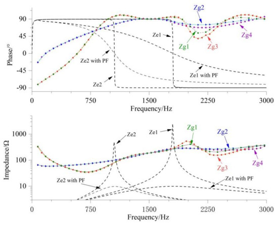
Figure 12.
Impedance–frequency curves of Cases 1–4.
After the passive filter is put into use in the traction network, the amplitude of Ze is reduced sharply, the phase change becomes flat at the same time, and the amplitude and phase conditions required for instability in (14) are destroyed, thus suppressing the harmonic overvoltage of the traction network.
The simulation result of Case 4 is shown in Figure 13. Before 0.22 s, Kci = 5. In this case, the condition of (14) is not satisfied, and there is no overvoltage in the traction network. Kci is increased to 40 at 0.22 s. According to the vehicle–grid impedance frequency characteristics shown in Figure 12, the condition of (14) is satisfied. Control instability occurs in the system, and the harmonic voltage of the traction network is continuously amplified as a divergent waveform. After 0.44 s, when the harmonic voltage of the traction network is amplified to a certain degree, it will not continue to be amplified, showing a steady-state waveform. The reason is that the amplitude limiting nonlinear segment of the control loop reduces the equivalent open-loop gain and forms a nonlinear self-excited oscillation process. In actual cases, nonlinear factors are more complicated. When the passive filter on the traction network side is put into operation after 0.6 s, the harmonic overvoltage disappears instantaneously.
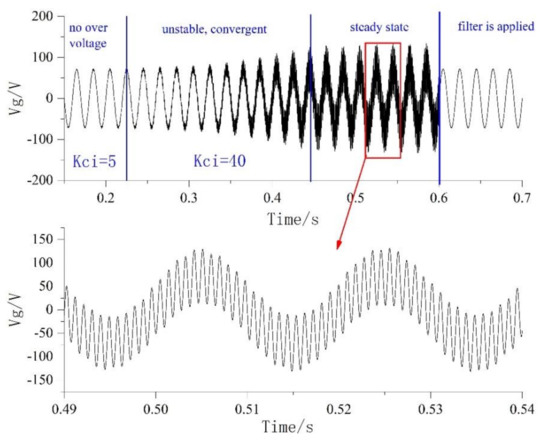
Figure 13.
Simulating waveforms of Case 4.
The impedance–frequency curves of Cases 5–7 are depicted in Figure 14 and the simulation result of Case 7 is shown in Figure 15. After applying the 9th-order harmonic disturbance of the current loop at 0.4 s, where analog is the output interference of the outer voltage loop. The high-order harmonic overvoltage appears in the voltage of the traction network, and the frequency of it is the same as the traction network inherent resonant frequency 1050 Hz. According to the impedance curve depicted in Figure 14, this system does not satisfy (14), hence, it is a stable system. However, harmonic overvoltage still occurs because at this time, fsam = 3000 Hz, whereas fsw = 750 Hz. Based on the sideband effect of modulation process mentioned in Section 4.2, the 9th-order low-harmonic will generate a high harmonic interference of 2 × 750 − 450 = 1050 Hz, which exactly coincides with the inherent resonant frequency of the TPSS (see curve Ze1 in Figure 12). Therefore, a traction network overvoltage occurs when the current is multiplied by extremely large impedance. The situation that controlled the stable vehicle–grid coupling system generates harmonic overvoltage in the traction network belonging to the second case discussed in (1). In this case, the grid-connected converter can be substituted by a harmonic current source model in the vehicle–grid coupling system.
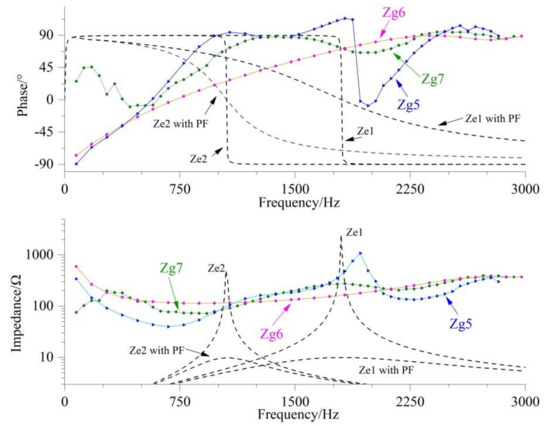
Figure 14.
Impedance–frequency curves of Cases 5–7.
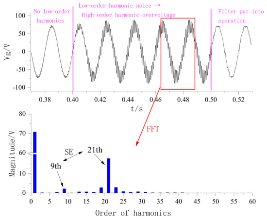
Figure 15.
Simulating waveforms of Case 7.
The limiting link of the control loop, as a nonlinear link, is equivalent to a gain reduction when the modulating wave is overmodulated. In future studies, we should consider the nonlinearity of the transformer hysteresis loop in the actual traction power system, which also has the effect of reducing the gain. In addition, we should consider other nonlinear conditions that occur in the actual line, which is our approach to be carried out in the future in this area.
7. Conclusions
In this paper, by studying the IFCs, sampling aliasing effect and modulation of the sideband effect model of the actual TPSSs, as well as considering the relative relationship of the inherent resonant frequency, sampling frequency and switching frequency of the TPSSs, harmonic overvoltage of traction network can be analyzed in a wide frequency range. Equation (1) is proposed to comprehensively elucidate the harmonic overvoltage mechanism of the traction network. The vehicle–grid coupling system instability model and the converter harmonic source model are unified and described in (1). Meanwhile, the application scope, distinction, and connection of these two models are discussed in detail.
Author Contributions
All authors contributed to the research in the paper. Conceptualization, M.W. and Q.L.; formal analysis, Q.L.; methodology, B.S. and Q.L.; project administration, M.W.; supervision, M.W.; validation, Q.Y.; writing—original draft, B.S.; writing—review and editing, T.H. and Q.L.; all the authors have read and approved the final manuscript. All authors have read and agreed to the published version of the manuscript.
Funding
This work was supported in part by the Fundamental Research Funds for the Central Universities (2020JBZD012) and the Project funded by China Postdoctoral Science Foundation (2020M670124).
Conflicts of Interest
The authors declare no conflict of interest.
References
- Song, K.; Mingli, W.; Yang, S.; Liu, Q.; Agelidis, V.G.; Konstantinou, G. High-Order Harmonic Resonances in Traction Power Supplies: A Review Based on Railway Operational Data, Measurements, and Experience. IEEE Trans. Power Electron. 2020, 35, 2501–2518. [Google Scholar] [CrossRef]
- Rodriguez-Diaz, E.; Freijedo, F.D.; Guerrero, J.G.M.; Marrero-Sosa, J.-A.; Dujic, D. Input-Admittance Passivity Compliance for Grid-Connected Converters With an LCL Filter. IEEE Trans. Ind. Electron. 2019, 66, 1089–1097. [Google Scholar] [CrossRef]
- Wang, Y.; Liu, S.; Liu, J. The stability criterion and damping control strategy for grid-connected inverters and its impact on the global system. Proc. CSEE 2020, 40, 3008–3020. [Google Scholar]
- Du, C.; Du, X.; Zou, X. Impedance modeling and stability analysis of grid-connected modular multilevel converter considering frequency coupling effect. Proc. CSEE 2020, 40, 2866–2876. [Google Scholar]
- Yang, R.; Zhou, F.; Zhong, K. A Harmonic Impedance Identification Method of Traction Network Based on Data Evolution Mechanism. Energies 2020, 13, 1904. [Google Scholar] [CrossRef]
- Zhou, F.; Liu, F.; Yang, R.; Liu, H. Method for Estimating Harmonic Parameters Based on Measurement Data without Phase Angle. Energies 2020, 13, 879. [Google Scholar] [CrossRef]
- European Standard. Railway Applications—Power Supply and Rolling Stock—Technical Criteria for the Coordination between Power Supply (Substation) and Rolling Stock to Achieve Interoperability; EN 50388:2012; European Electro Technical Standardization Committee: Brussels, Belgium, 2012. [Google Scholar]
- Harnefors, L.; Finger, R.; Wang, X.; Bai, H.; Blaabjerg, F. VSC Input-Admittance Modeling and Analysis above the Nyquist Frequency for Passivity-Based Stability Assessment. IEEE Trans. Ind. Electron. 2017, 64, 6362–6370. [Google Scholar] [CrossRef]
- Freijedo, F.D.; Ferrer, M.; Dujic, D.; Ferrer-Duran, M. Multivariable High-Frequency Input-Admittance of Grid-Connected Converters: Modeling, Validation, and Implications on Stability. IEEE Trans. Ind. Electron. 2019, 66, 6505–6515. [Google Scholar] [CrossRef]
- Liu, M.; Wei, Q.; Xie, S.; Qian, Q.; Zhang, Z.; Xu, J. Multifrequency Impedance Model of Single-Phase Grid-Connected Parallel Inverters for Analysis on Circulating Resonant Current. In Proceedings of the 2019 IEEE Energy Conversion Congress and Exposition (ECCE), Baltimore, MD, USA, 29 September–3 October 2019; pp. 3655–3658. [Google Scholar]
- Yang, J.; Liu, J.; Shi, Y.; Zhao, N.; Zhang, J.; Fu, L.; Zheng, T.Q. Carrier-Based Digital PWM and Multirate Technique of a Cascaded H-Bridge Converter for Power Electronic Traction Transformers. IEEE J. Emerg. Sel. Top. Power Electron. 2019, 7, 1207–1223. [Google Scholar] [CrossRef]
- Zhou, F.; Xiong, J.; Zhong, K. Research on the phenomenon of the locomotive converter output current spectrum move based on the coupling of the train net system. Proc. CSEE 2018, 38, 1818–1825. [Google Scholar]
- Cui, H.; Feng, Y.; Lin, X. Simulation study of the harmonic resonance characteristics of the coupling system with a traction network and AC-DC-AC trains. Proc. CSEE 2014, 34, 2736–2745. [Google Scholar]
- Liu, Q.; Wu, M.; Li, J.; Yang, S. Frequency-Scanning Harmonic Generator for (Inter)harmonic Impedance Tests and Its Implementation in Actual 2 × 25 kV Railway Systems. IEEE Trans. Ind. Electron. 2020. [Google Scholar] [CrossRef]
- Liu, Q. Research on Impedance-Frequency Characteristic Test Technology of Traction Power Supply Systems. Ph.D. Thesis, Beijing Jiaotong University, Beijing, China, 2018. [Google Scholar]
- Mouton, H.D.T.; McGrath, B.; Holmes, D.G.; Wilkinson, R.H. One-Dimensional Spectral Analysis of Complex PWM Waveforms Using Superposition. IEEE Trans. Power Electron. 2014, 29, 6762–6778. [Google Scholar] [CrossRef]
- Hans, F.; Oeltze, M.; Schumacher, W. A Modified ZOH Model for Representing the Small-Signal PWM Behavior in Digital DC-AC Converter Systems. In Proceedings of the IECON 2019 45th Annual Conference of the IEEE Industrial Electronics Society, Lisbon, Portugal, 14–17 October 2019; Volume 1, pp. 1514–1520. [Google Scholar]
- Liu, Q.; Wu , M.; Li, J.; Zhang, J. Controllable harmonic generating method for harmonic impedance measurement of traction power supply systems based on phase shifted PWM. J. Power Electron. 2018, 18, 1140–1153. [Google Scholar]
Publisher’s Note: MDPI stays neutral with regard to jurisdictional claims in published maps and institutional affiliations. |
© 2020 by the authors. Licensee MDPI, Basel, Switzerland. This article is an open access article distributed under the terms and conditions of the Creative Commons Attribution (CC BY) license (http://creativecommons.org/licenses/by/4.0/).