A Computational Workflow for Flow and Transport in Fractured Porous Media Based on a Hierarchical Nonlinear Discrete Fracture Modeling Approach

Abstract

Modeling flow and transport in fractured porous media has been a topic of intensive research for a number of energy- and environment-related industries. The presence of multiscale fractures makes it an extremely challenging task to resolve accurately and efficiently the flow dynamics at both the local and global scales. To tackle this challenge, we developed a computational workflow that adopts a two-level hierarchical strategy based on fracture length partitioning. This was achieved by specifying a partition length to split the discrete fracture network (DFN) into small-scale fractures and large-scale fractures. Flow-based numerical upscaling was then employed to homogenize the small-scale fractures and the porous matrix into an equivalent/effective single medium, whereas the large-scale fractures were modeled explicitly. As the effective medium properties can be fully tensorial, the developed hierarchical framework constructed the discrete systems for the explicit fracture–matrix sub-domains using the nonlinear two-point flux approximation (NTPFA) scheme. This led to a significant reduction of grid orientation effects, thus developing a robust, applicable, and field-relevant framework. To assess the efficacy of the proposed hierarchical workflow, several numerical simulations were carried out to systematically analyze the effects of the homogenized explicit cutoff length scale, as well as the fracture length and orientation distributions. The effect of different boundary conditions, namely, the constant pressure drop boundary condition and the linear pressure boundary condition, for the numerical upscaling on the accuracy of the workflow was investigated. The results show that when the partition length is much larger than the characteristic length of the grid block, and when the DFN has a predominant orientation that is often the case in practical simulations, the workflow employing linear pressure boundary conditions for numerical upscaling give closer results to the full-model reference solutions. Our findings shed new light on the development of meaningful computational frameworks for highly fractured, heterogeneous geological media where fractures are present at multiple scales.

1. Introduction

Modeling fluid flow and transport in fractured porous media on the field scale, both accurately and efficiently, has been a long-standing issue in a number of energy- and environment-related disciplines, such as production of oil and gas from naturally fractured reservoirs, extraction of geothermal energies, disposal of nuclear waste underground, sequestration of carbon dioxide in deep saline reservoirs, just to name a few. As a result, numerous conceptual and numerical models have been proposed over the years (see a recent review by Berre et al. [1] and the references therein). Broadly speaking, the models can be classified into the following three categories: equivalent/effective medium models, multi-continuum models and discrete fracture–matrix (DFM) models. The equivalent/effective medium models assume that fractures and the surrounding porous matrix are in equilibrium at all times. As such, the matrix and fracture properties are all lumped into single equivalent (effective) properties. This single-medium model facilities efficient numerical simulations as conventional reservoir simulators can be used directly without many modifications. Its applications, however, may be limited by its overly simplified assumptions. The multi-continuum models, notably the dual-continuum models such as dual-porosity/dual-permeability, conceptualize the whole system as two separate yet interacting continua. This model was first proposed in [2] and was introduced to the petroleum industry by Warren and Root [3]. Based on this concept, numerous reservoir simulators were developed to model multiphase flow in naturally fractured reservoirs [4,5,6]. A key element in these models is the so-called transfer functions that encompass a geometric shape factor. Transfer functions and shape factors received an enormous interest throughout the years as is evident in the large body of literature (see, e.g., [7,8,9] and the references therein). The multi-continuum models represent a significant step forward and have become the method of choice for many years. However, they are most applicable for densely fractured reservoirs and are inadequate for capturing the dominant effects of large highly conductive fractures. Moreover, a rigorous definition of the transfer function for multiple physics can be quite problematic. Unlike the equivalent or multi-continuum models, the DFM models assume a complete knowledge of the discrete fracture network (DFN) and each fracture is modeled explicitly [10,11]. The DFM models are considered to be the most physically realistic, yet they suffer from prohibitive computational expenses and cannot be deployed on the field scale. For example, the discrete fracture–matrix (DFM) models usually require an unstructured mesh that conforms to the fracture geometries, which poses significant challenges for densely fractured reservoirs and often results in an excessive number of cells in the mesh. The meshing difficulties can be circumvented by using a class of embedded discrete fracture–matrix (EDFM) models [12,13], which discretize the porous matrix independently without considering the presence of fractures. Fracture control volumes are then formed naturally from their intersection with matrix–cell boundaries. Non-neighboring connections (NNCs) are introduced to connect the fracture control volumes to the porous matrix. Despite its efficiency in meshing, the inclusion of all the discrete fractures can still lead to an overly large discretized system and the introduction of a large number of NNCs can also deteriorate the performance of linear solvers, slowing down simulations as a result.

Considering that large-scale fractures can have a leading dominant role in flow behavior in a fractured reservoir while the effects of small-scale fractures are mainly local, a realistic option is to homogenize the small-scale fractures and explicitly model the large-scale fractures only. The small-scale fractures can be homogenized into a continuum on its own, leading to dual-porosity models. Alternatively, they can be upscaled together with the rock matrix into an equivalent medium, resulting in single-porosity models. This idea of hierarchical modeling of fractures was explored in [14,15], where the fractures are classified as short, medium, and long fractures based on the ratio of the fracture length to the characteristic length of the grid blocks. The short and medium fractures are homogenized into the rock matrix to derive an equivalent permeability tensor, whereas the large fractures are modeled explicitly. To determine whether a fracture is large or not, based on its length, requires a partition length scale. Fractures with lengths larger than the partition length should be modeled explicitly, whereas fractures whose length is less than the partition length can be upscaled. In a more recent work [16], the authors investigated the relationship between the upscaled effective permeability and the partition length and concluded that there is a threshold partition length beyond which the upscaled effective permeability increases rapidly. Numerical flow-based upscaling was used in their work to compute the upscaled effective permeability. An important component of numerical upscaling is the selection of boundary conditions, and the authors of [16] chose a set of boundary conditions that gives rise to diagonal equivalent/effective permeability tensors, which yields some convenience for two-point flux approximation (TPFA)-based simulators. In practice, a full permeability tensor with non-zero off-diagonal elements may be more appropriate to represent the flow properties of the rock matrix together with the small-scale fractures as the DFNs often have a predominant orientation because of the state of the stress field when the fractures were formed.

In this work, we follow similar ideas presented in [16] and build a computational workflow for modeling flow and transport in fractured porous media. The aim of this research was to investigate and compare the effect of different boundary conditions on the upscaling of small-scale fractures. Specifically, we considered the constant pressure drop boundary condition that gives rise to a diagonal equivalent/effective tensor and the linear pressure boundary condition that leads to a full tensor with non-zero off-diagonal elements. Once the small-scale fractures were upscaled, the large-scale fractures were modeled explicitly using the EDFM model. To solve the flow equation consistently when the upscaled permeability was a full tensor, a monotone nonlinear two-point flux approximation (NTPFA) [17] method was used so that the comparative results were not distorted by numerical discretization errors.

2. Modeling Methods

2.1. Description of the Modeling Workflow

The modeling workflow is illustrated in Figure 1. Given the computational grid and DFN, as shown in Figure 1a, a partition length $l_{\mathrm{p}}$ is defined to classify all fractures into 2 sets. Fractures whose lengths are smaller than $l_{\mathrm{p}}$ are classified as small-scale fractures, whereas all others are classified as large-scale fractures. An illustration is provided in Figure 1b,c. Numerical flow-based upscaling is then used to homogenize the small-scale fractures with the rock matrix, resulting in equivalent permeability tensors for the matrix grid blocks shown in Figure 1d, where the equivalent permeability tensors are represented by ellipses whose semi-axes are scaled by the square root of the principal values of the tensors. The large-scale fractures are, however, modeled explicitly, as shown in Figure 1e. Depending on the local boundary conditions, used for numerical upscaling (homogenization), diagonal or full permeability tensors are obtained. The linear flux approximation scheme, i.e., TPFA, is used to discretize the flow equation if the upscaled tensor is found to be diagonal, and the NTPFA method is used if the upscaled permeability is a full tensor. Note that this leads to an adaptive framework, in which NTPFA is applied only when it is necessary. For both cases, as shown in Figure 1e, the EDFM method is used to model the large-scale fractures along with the heterogeneous matrix rock.

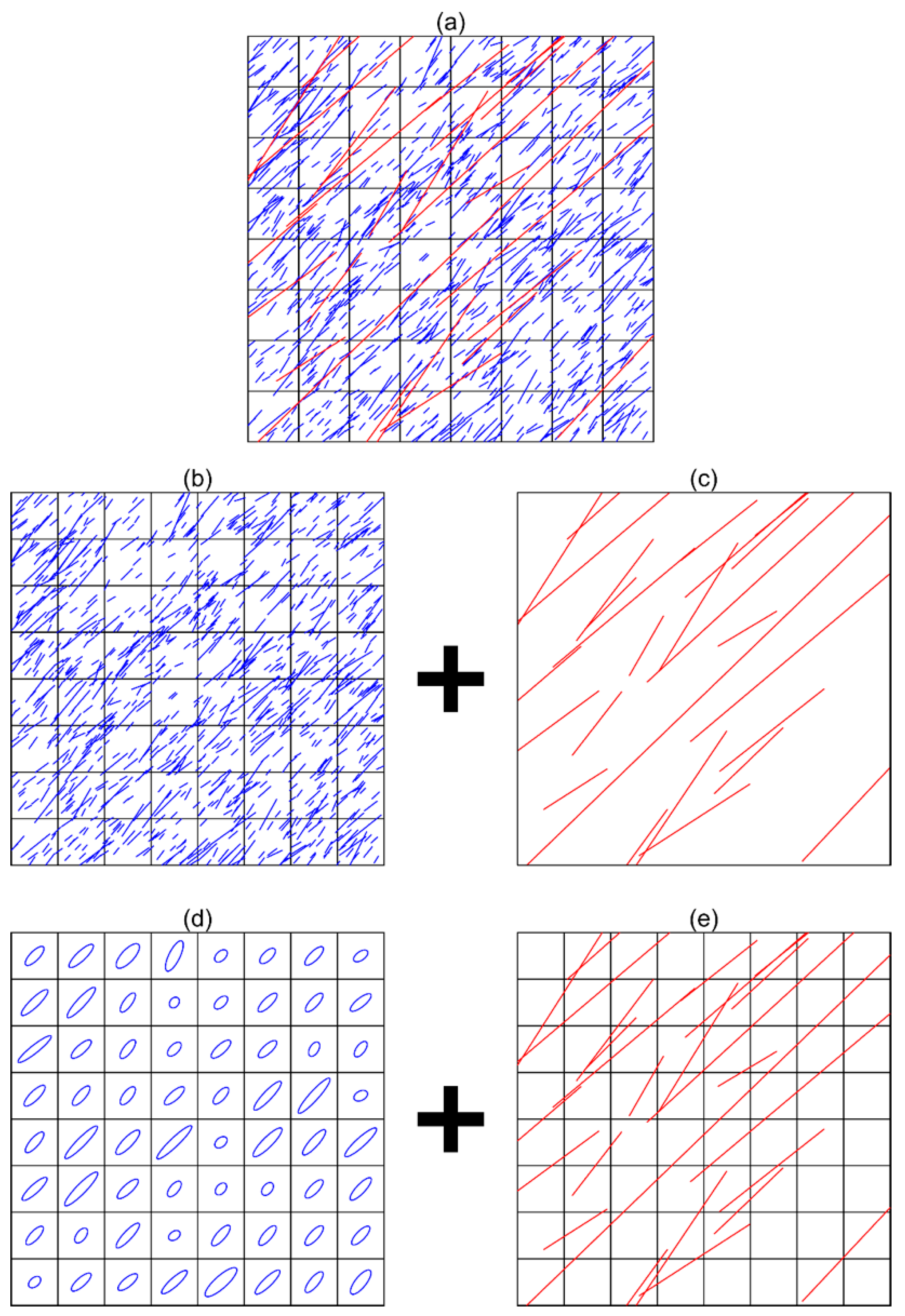
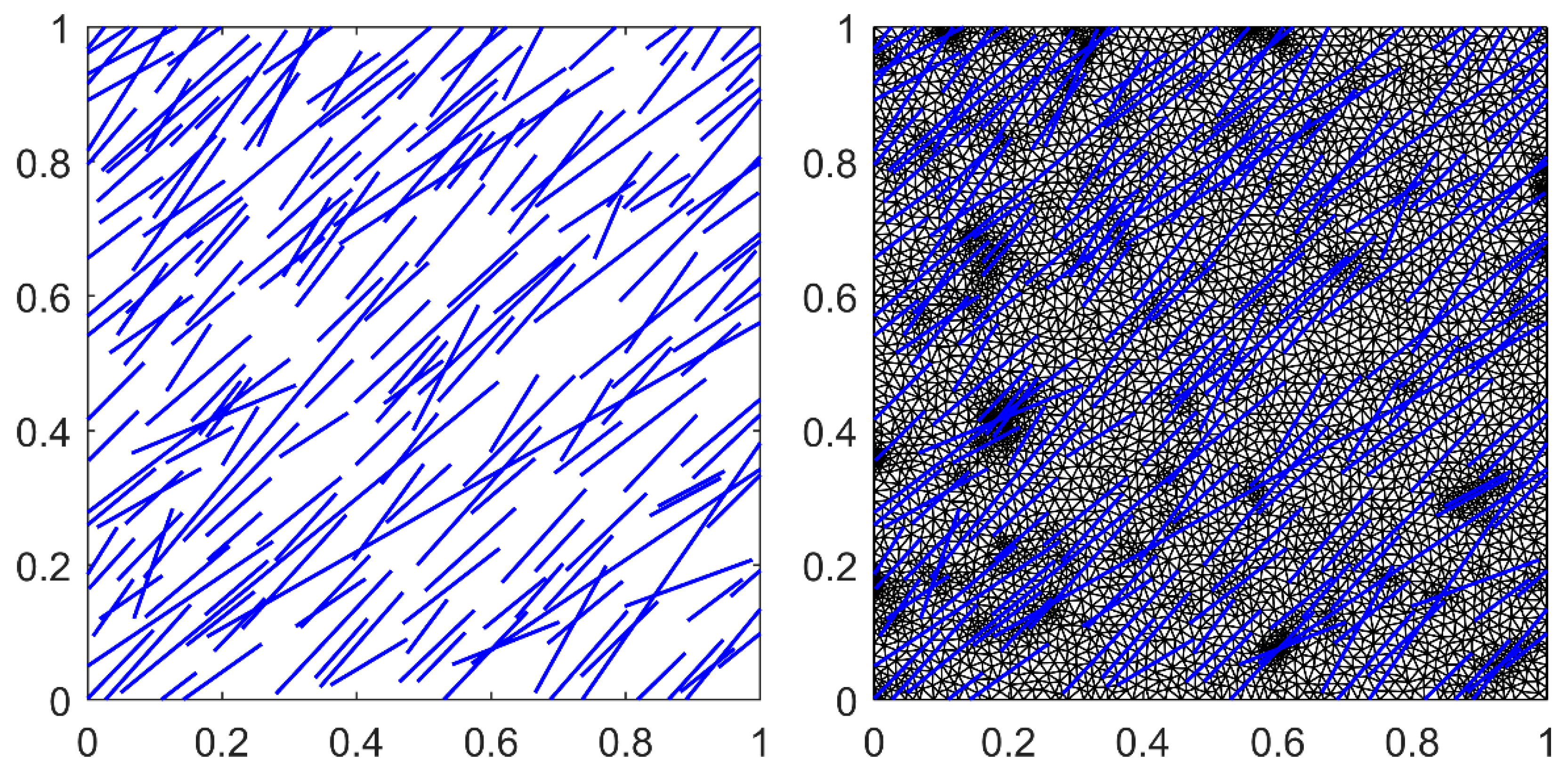
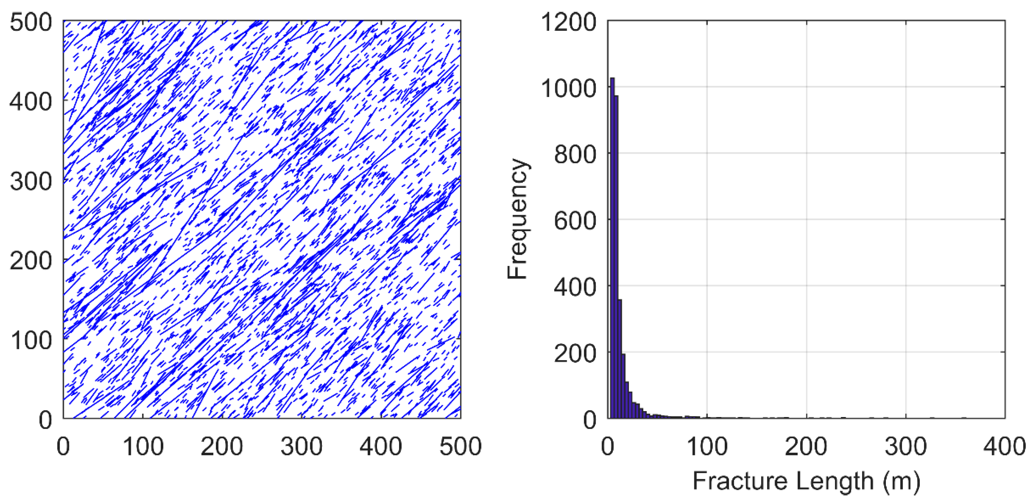
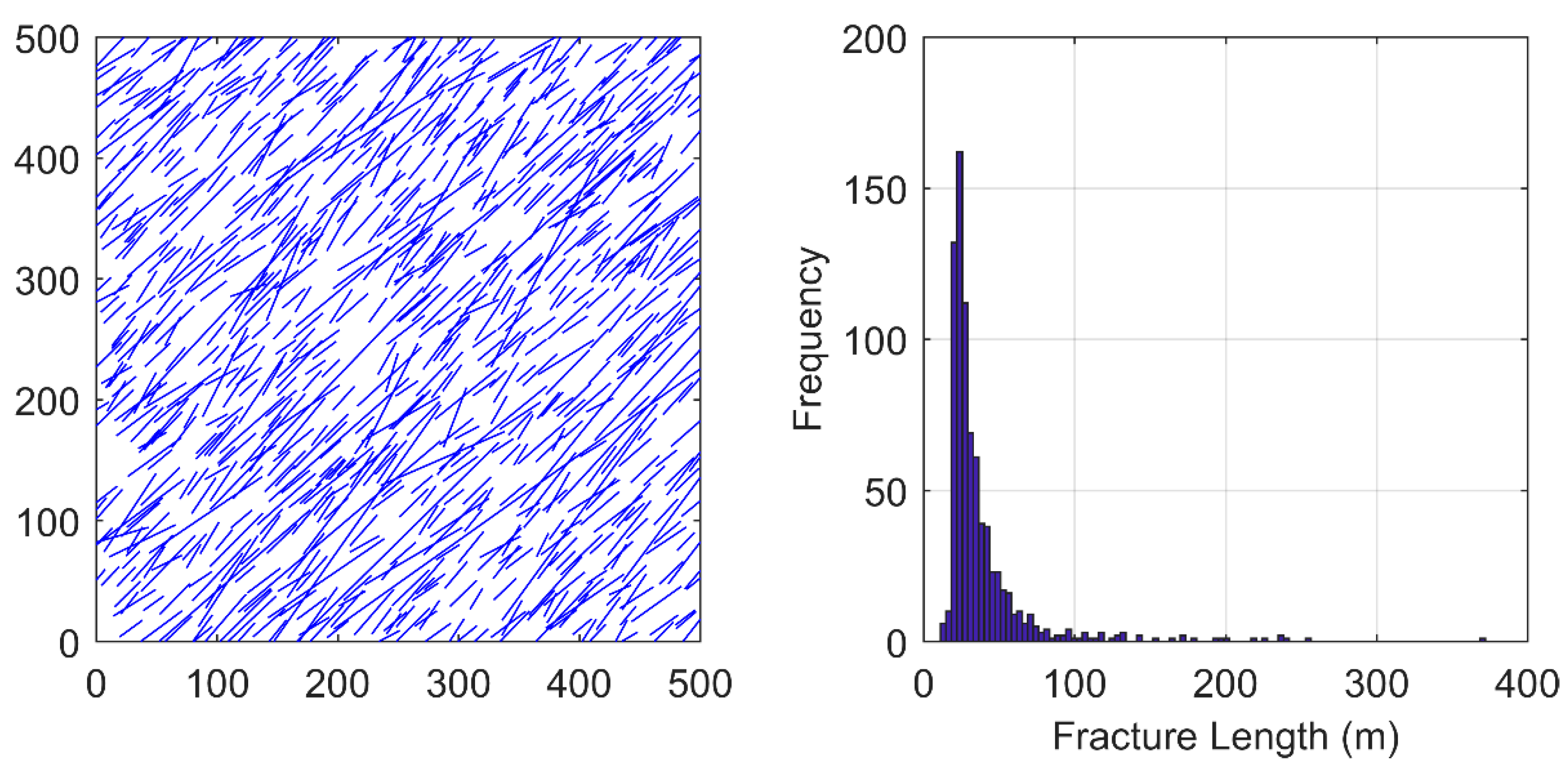
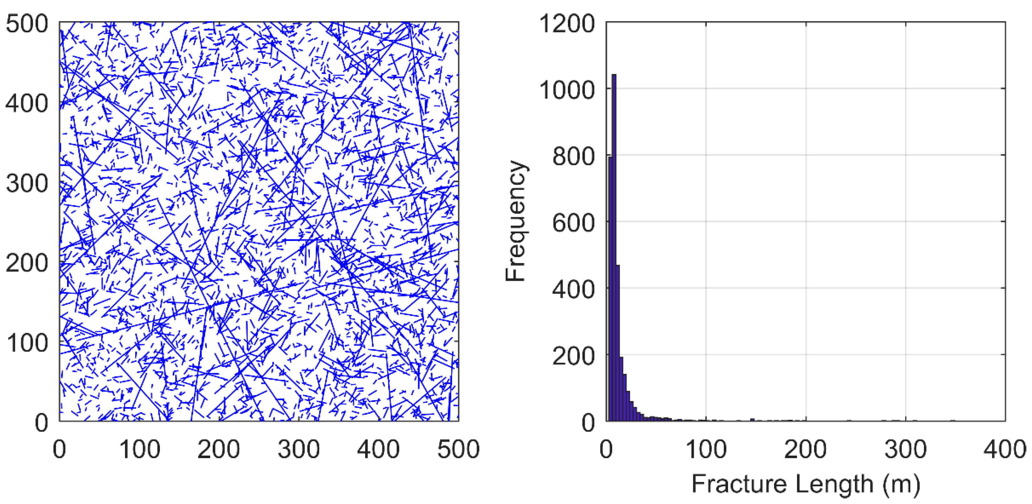
2.2. Discrete Fracture Network (DFN) Generation

The DFNs are generated stochastically by drawing samples randomly from specified distributions. Each fracture segment can be characterized by three parameters, namely, its location (the centroid of the line segment ${\mathit{x}}_{\mathrm{c}}$), orientation ($\theta$), and length ($l$). We assume that the distributions of the three parameters are independent. The fracture location ${\mathit{x}}_{\mathrm{c}}$ is assumed to follow the uniform distribution. The von Mises distribution is used for fracture orientation $\theta$. The von Mises distribution is an analogue of the normal distribution for circular data and its probability density distribution function is given by [18] as follows:

$$f_{\mathsf{\Theta }}\left(\theta ;\mu ,\kappa \right)=\frac{1}{2\pi I_0\left(\kappa \right)}\exp \left(\kappa \cos \left(\theta -\mu \right)\right),$$

(1)

where $\theta \in \left[0, 2\pi \right)$. Moreover, $I_0$ is the modified Bessel function of the first kind of order zero, and $\mu$ is the distribution mean. The variance of the distribution is given by ${\sigma }^2=1-\frac{I_1\left(\kappa \right)}{I_0\left(\kappa \right)}$. The greater the value of $\kappa$, the smaller the variance. The fracture length $l$ is often characterized by a positive skewed distribution that has a long tail on the right such as the negative exponential distribution, log-normal distribution, power-law distribution, etc. In this work, the power-law distribution is used to describe the fracture length statistics although other distributions can be used as well. The probability density function for power-law distribution is given by [19] as follows:

$$f_L\left(l;\alpha ,l_{\min }, l_{\max }\right)=C{l}^{-\alpha },$$

(2)

where $l\in \left[l_{\min }, l_{\max }\right]$. $l_{\min }$ and $l_{\max }$ are the minimum and maximum lengths of the fractures, respectively. In addition, $\alpha$ is the exponent that is greater than 1 and $C$ is a normalization constant. Integrating Equation (2) from $l_{\min }$ to $l_{\max }$ gives the following:

$${{\displaystyle \int }}_{l_{\min }}^{l_{\max }}C{l}^{-\alpha }=C\frac{1}{-\alpha +1}{l}^{-\alpha +1}|\begin{array}{c}a\\ \\ b\end{array}=1$$

(3)

Solving Equation (3) for the normalization constant results in $C=\frac{-\alpha +1}{l_{\max }^{-\alpha +1}-l_{\min }^{-\alpha +1}}$. Note that the stochastically generated DFN is cropped onto a given domain by cutting fractures that intersect the boundary of the domain. Therefore, the actual minimum and maximum fracture lengths are different from the two parameters $l_{\min }$ and $l_{\max }$.

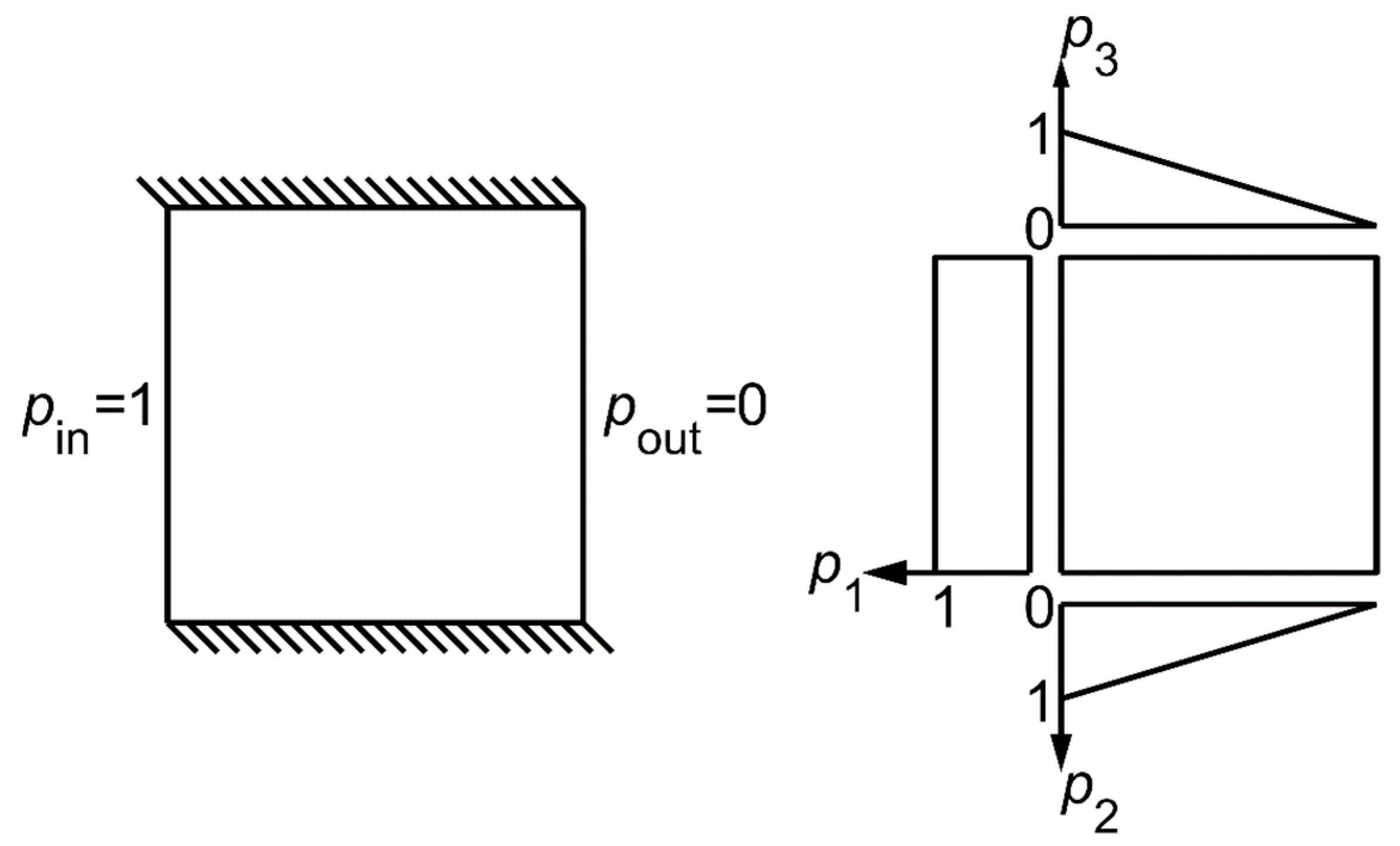
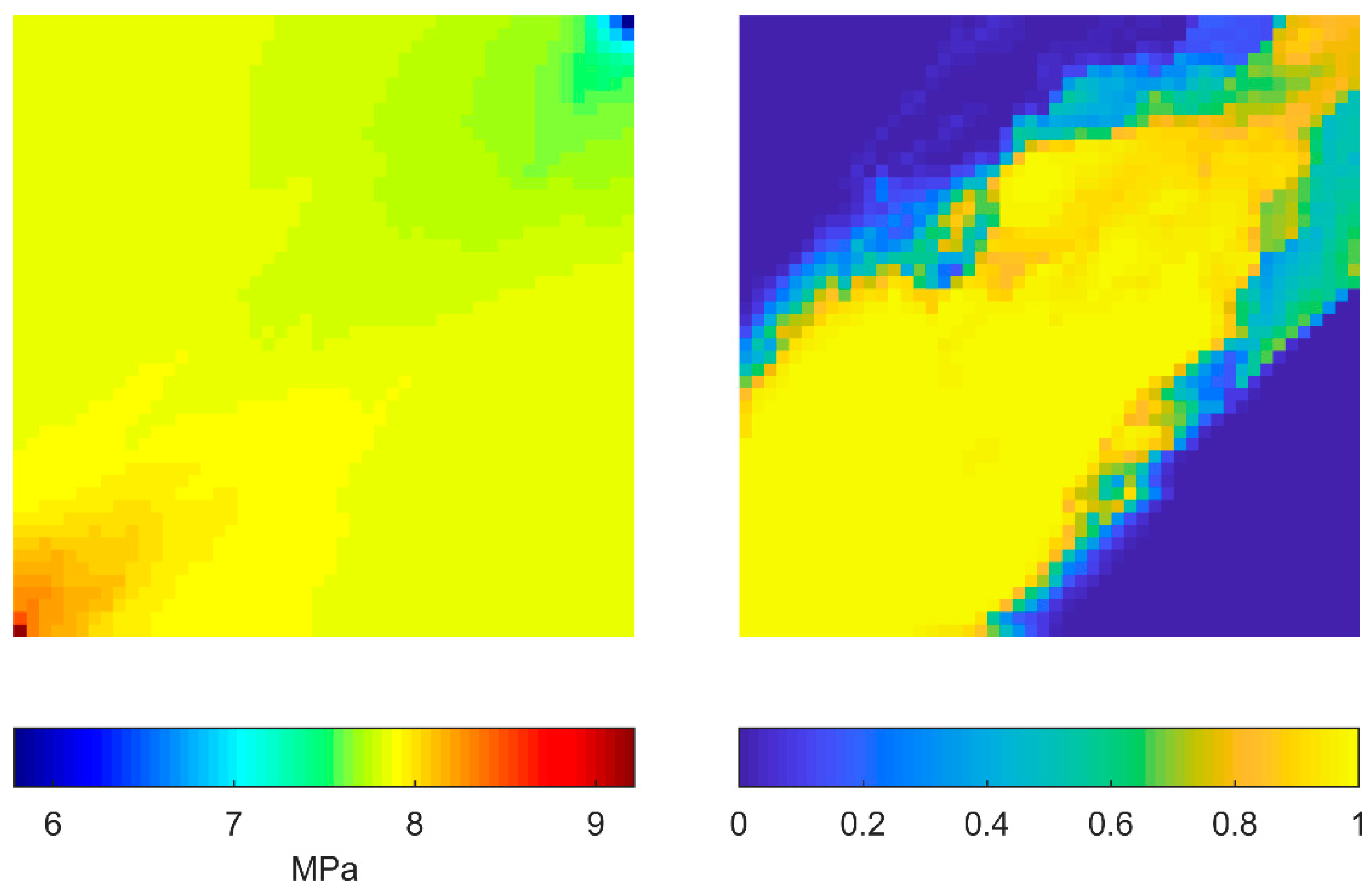
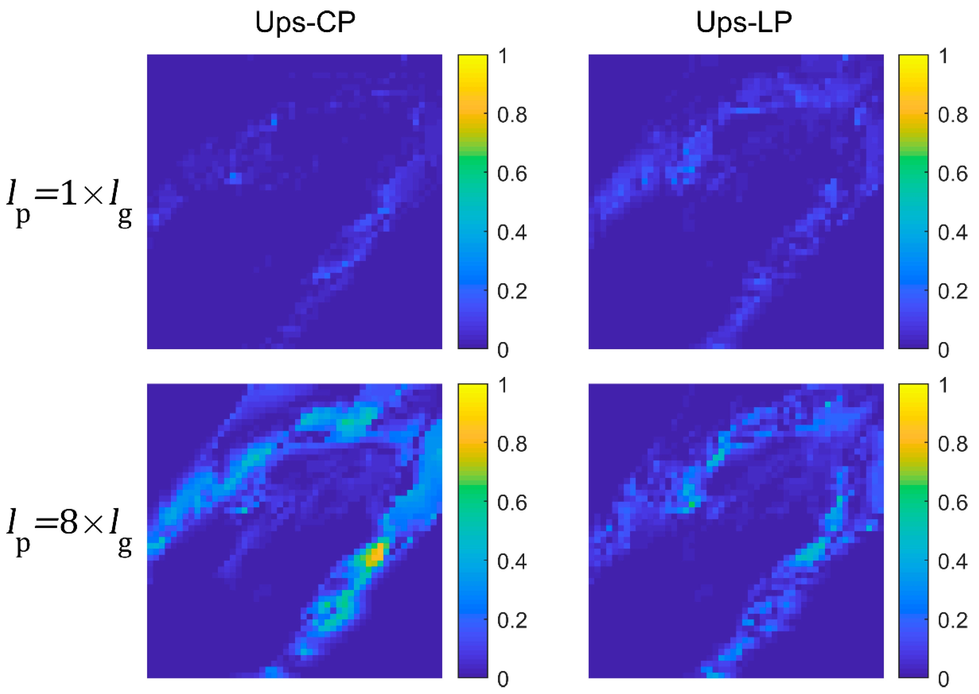
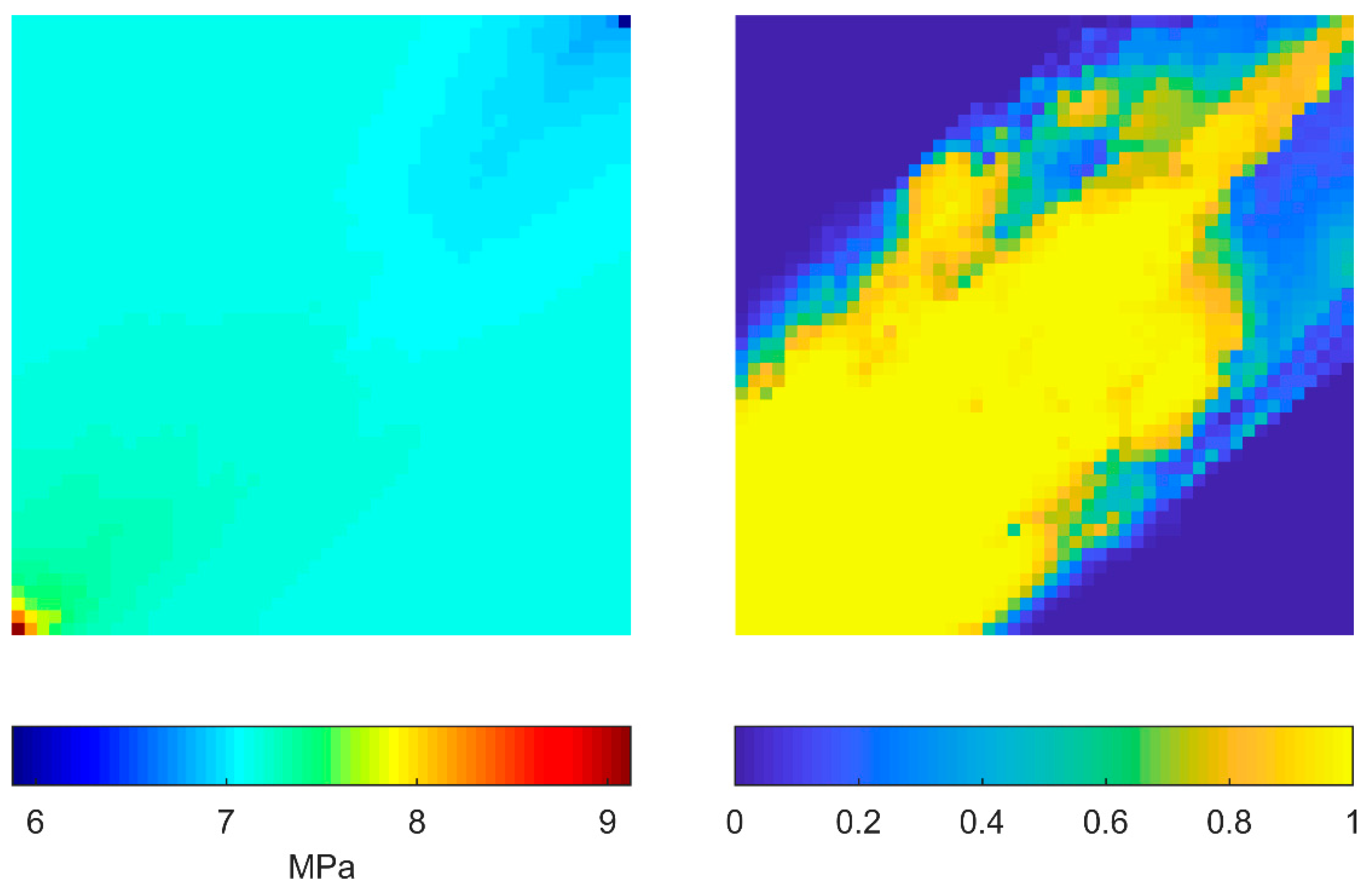
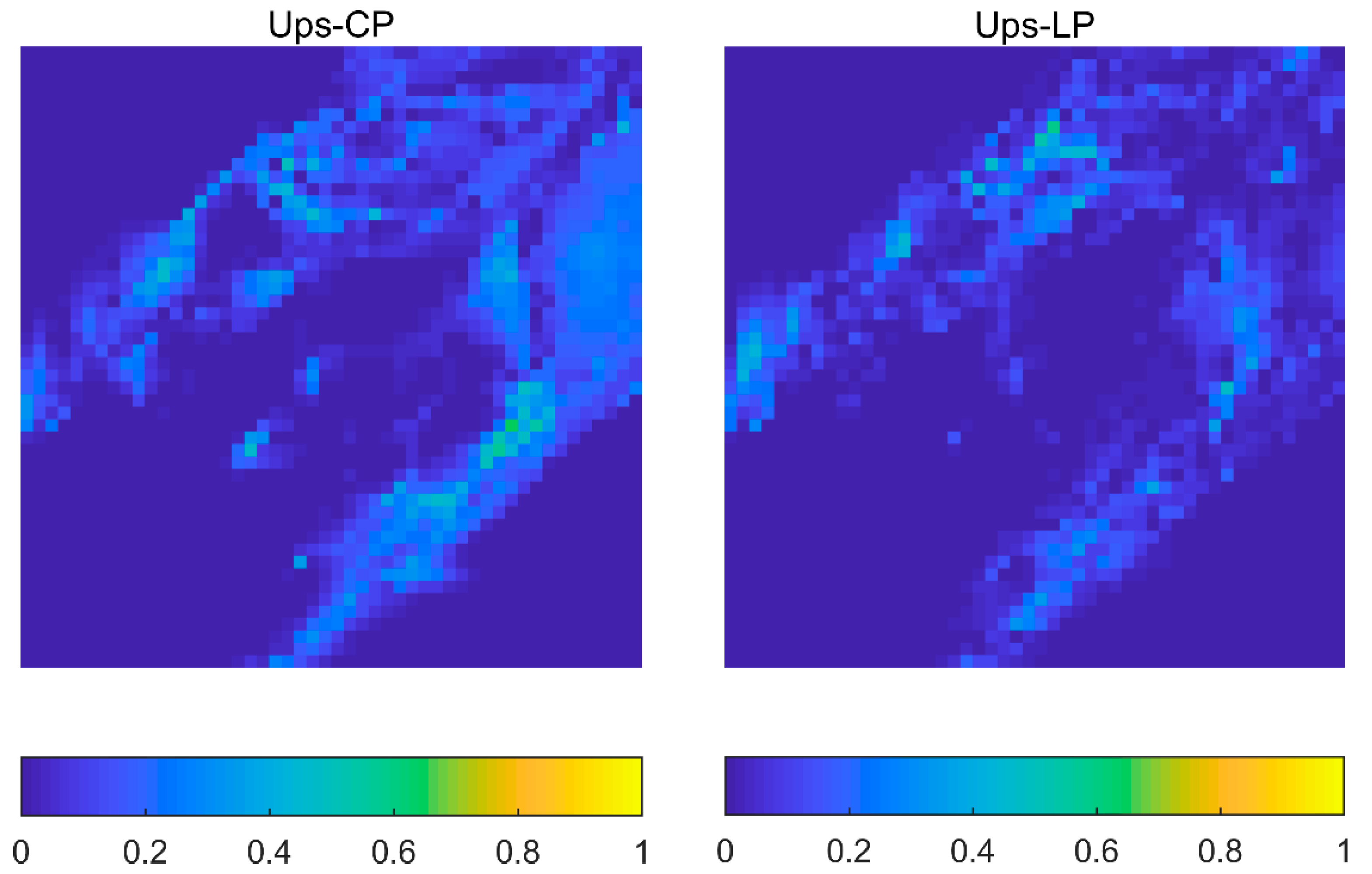
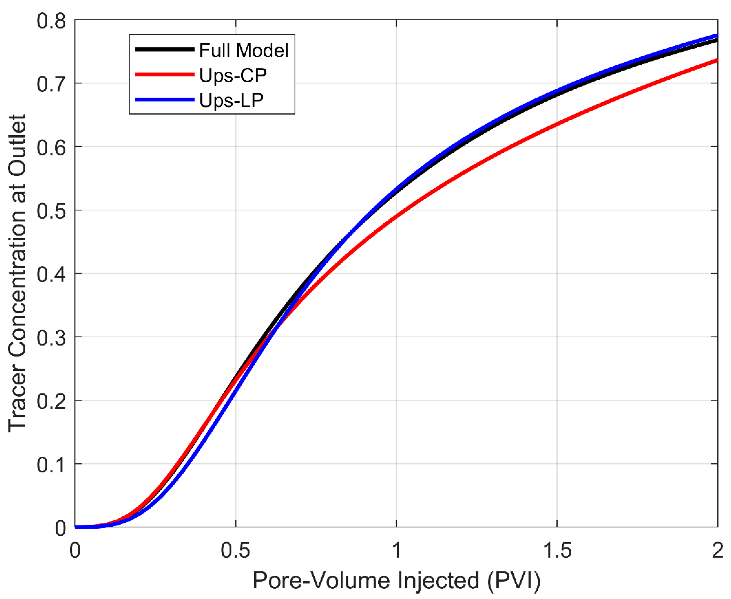
2.3. Numerical Upscaling

There is a tremendous amount of literature devoted to the subject of upscaling. For the following, we used the techniques presented in [20] and the references therein. Numerically upscaling small-scale fractures with the rock matrix entails solving the incompressible single-phase flow equation on the domain of question. Different upscaling results can be obtained by using different boundary conditions. We considered two types of boundary conditions, namely, constant pressure drop (CP) and linear pressure (LP) boundary conditions. The most common boundary condition is the constant pressure drop on a pair of opposing faces and no-flow boundary conditions on the remaining faces as shown in the left of Figure 2. Suppose that the physical dimension of the grid block to be upscaled is $L_x, L_y$ in the $x, y$ direction, respectively, for a 2D problem. To compute an equivalent permeability in the $x$ direction, an incompressible single-phase flow problem is solved with a constant pressure drop in the $x$ direction while the remaining boundary faces are closed to flow. Upon computing the total flux $Q_x$ in the $x$ direction, the equivalent permeability $k_x^{*}$ in the $x$ direction is related to $Q_x$ by Darcy’s law as follows:

$$Q_x=\frac{k_x^{*}{A}_x\Delta p}{\mu L_x}=\frac{k_x^{*}{L}_y}{\mu L_x}\left(p_{\mathrm{in}}-p_{\mathrm{out}}\right),$$

(4)

where $\mu$ is fluid viscosity, $A_x$ is the cross-section area for flow in the $x$ direction and is numerically equal to $L_y$ in 2D, and $\Delta p$ is the pressure drop. Solving for $k_x^{*}$ gives the following:

$$k_x^{*}=\frac{\mu Q_x{L}_x}{L_y\left(p_{\mathrm{in}}-p_{\mathrm{out}}\right)}=\frac{\mu Q_x{L}_x}{L_y\left(p_{\mathrm{in}}-p_{\mathrm{out}}\right)}.$$

(5)

In actual implementation, the fluid viscosity $\mu$ can be taken as unity and $p_{\mathrm{in}}=1, p_{\mathrm{out}}=0$ for simplicity. Then $k_x^{*}$ is equal to $Q_x{L}_x/L_y$. The equivalent permeability $k_y^{*}$ in the $y$ direction can be computed similarly by imposing a constant pressure drop in the $y$ direction. Applying the boundary condition of constant pressure drop results in an equivalent permeability that is diagonal. Thus, the classical linear two-point flux approximation (TPFA) method can be used for solving the flow equation for the upscaled model. For brevity, this type of upscaled model is denoted by “Ups-CP”.

Considering the fact that the discrete fracture network usually has a predominant orientation because of the state of the stress field when the fractures were formed, it may be more appropriate to represent the homogenized media by full permeability tensors with non-zero off-diagonal elements. Therefore, we also applied the linear boundary condition for upscaling, as shown in the right of Figure 2. If the matrix domain and the small-scale fractures contained within it behave as a homogeneous anisotropic media with an equivalent permeability tensor $K^{*}$, then Darcy’s equation can be written in a component-wise form as follows:

$$\left[\begin{array}{c}{v}_x\\ v_y\end{array}\right]=-\frac{1}{\mu }\left[\begin{array}{cc}{k}_{xx}^{*}& k_{xy}^{*}\\ k_{yx}^{*}& k_{yy}^{*}\end{array}\right]\left[\begin{array}{c}\frac{\partial p}{\partial x}\\ \frac{\partial p}{\partial y}\end{array}\right],$$

(6)

where $v_x, v_y$ are components of the Darcy velocity in the $x,y$ directions, respectively. $k_{xx}^{*}, k_{xy}^{*}, k_{yx}^{*}, k_{yy}^{*}$ are the components of K*. The total flux in the $x, y$ direction for single-phase flow is then given by the following:

$$\begin{array}{c}{Q}_x=-\frac{A_x}{\mu }\left(k_{xx}^{*}\frac{\partial p}{\partial x}+k_{xy}^{*}\frac{\partial p}{\partial y}\right)\\ Q_y=-\frac{A_y}{\mu }\left(k_{yx}^{*}\frac{\partial p}{\partial x}+k_{yy}^{*}\frac{\partial p}{\partial y}\right)\end{array}$$

(7)

To compute the components of K*, a linear pressure boundary condition $p\left(x,y\right)=1-\frac{x}{L_x}$ is applied on all the boundary faces of the domain and the incompressible single-phase flow equation is solved. Integrating the Darcy velocity along the respective boundaries gives the total flux $Q_x, Q_y$. Assuming that the pressure distribution inside the domain is also linear and is consistent with the boundary conditions, we can compute the components of the pressure gradient as $\frac{\partial p}{\partial x}=-\frac{1}{L_x}$ and $\frac{\partial p}{\partial y}=0$. Substituting the total flux and pressure gradient into Equation (7) and solving for $k_{xx}^{*}, k_{yx}^{*}$ leads to the following:

$$\begin{array}{c}{k}_{xx}^{*}=\frac{\mu Q_x{L}_x}{A_x}=\frac{L_x}{L_y}{Q}_x\\ k_{yx}^{*}=\frac{\mu Q_y{L}_x}{A_y}=\frac{L_x}{L_x}{Q}_y=Q_y\end{array}$$

(8)

where, similar as before, the fluid viscosity is unity. Repeating the same procedure and replacing the boundary condition by $p\left(x,y\right)=1-\frac{y}{L_y}$, we can compute the values of $k_{xy}^{*}$ and $k_{yy}^{*}$. One issue with this upscaling approach is that the total fluxes $Q_x, Q_y$ are not uniquely found across the local domain. For example, the total flux computed across the left boundary $Q_{x1}$ can be different than the one computed across the right boundary $Q_{x2}$. For homogeneous isotropic local domains, the two values are close to each other. However, they can differ significantly for heterogeneous anisotropic domains, which is especially true of fractured porous media. In this work, we computed the total flow rates in the x and y directions, i.e., $Q_x$ and $Q_y$, as the average of their corresponding end boundaries. More precisely, $Q_x=\frac{Q_{x1}+Q_{x2}}{2}$ and $Q_y=\frac{Q_{y1}+Q_{y2}}{2}$. The upscaled full permeability tensors are used to solve the flow equations globally using the nonlinear finite volume method (NTPFA). Derivation of the nonlinear finite volume methods, however, requires that the permeability tensor be symmetric and positive-definite (SPD). The upscaled permeability tensor using the linear pressure boundary condition cannot be guaranteed to be either symmetric or positive-definite. For example, it is not difficult to see that the cross-terms $k_{xy}^{*}, k_{yx}^{*}$ are not equal in general. To enforce symmetry, the final upscaled permeability tensor can be taken as $\frac{\left(K^{*}+{\left(K^{*}\right)}^{\mathrm{T}}\right)}{2}$, where the superscript T denotes the transpose. The property of being positive-definite is more difficult to achieve. To circumvent this problem, we checked the positive-definiteness of the upscaled permeability tensor for each upscaled grid block. If it was not positive-definite, we replaced the upscaled permeability with the diagonal tensor by applying the constant pressure drop boundary conditions. Therefore, this second type of upscaled model is actually a hybrid model that utilizes both types of boundary conditions depending on the upscaling results. We refer to this model as “Ups-LP” hereafter.

To solve the incompressible single-phase flow in a fractured porous medium, either the DFM or EDFM models can be used. On the one hand, DFM models require the mesh to conform to the fracture geometries, and unstructured triangular meshes are needed in general. As a result, the mesh may not be K-orthogonal even for isotropic matrix permeability and the linear TPFA method will be inconsistent. Therefore, we used the nonlinear TPFA method for DFM models [21,22], and we denote it by “DFM-NTPFA. EDFM models, on the other hand, work on a Cartesian mesh and the linear TPFA is adequate if the matrix permeability is isotropic. We denote this method by “EDFM-TPFA”. The left plot of Figure 3 shows an example of a stochastically generated DFN that has a predominant orientation from the northeast to the southwest on the unit square and the corresponding unstructured triangular mesh is shown in the right of the figure. As can be seen, very fine meshes are needed around fractures to conform to their geometry, especially near fracture intersections. The total number of cells in the mesh is 11,448. Figure 4 shows the pressure distribution of DFM-NTPFA and EDFM-TPFA for the linear pressure boundary condition $p\left(x,y\right)=1-x$. The EDFM-TPFA model is solved on a uniform $70\times 70$ Cartesian mesh. There is a very close agreement in the pressure solutions between the two methods.

Table 1. Total flux in $x,y$ directions using discrete fracture-matrix–nonlinear two-point flux approximation (DFM-NTPFA) and embedded discrete fracture–matrix–two-point flux approximation (EDFM-TPFA) methods corresponding to the results of Figure 4.

	${\mathit{Q}}_{\mathit{x}1}$	${\mathit{Q}}_{\mathit{x}2}$	${\mathit{Q}}_{\mathit{y}1}$	${\mathit{Q}}_{\mathit{y}2}$
DFM-NTPFA	55.0631	32.6250	27.7312	50.1693
EDFM-TPFA	55.6896	33.5183	27.9913	50.1626

lists the total flux in the $x,y$ directions computed from the flow solutions of the two methods, and we can see that the results are in excellent agreement. We conducted a series of numerical tests with different realizations of DFNs and found that the results of EDFM-TPFA are quite close to those of DFM-NTPFA for engineering purposes. Therefore, in the following, only the EDFM-TPFA method is used for upscaling as it is computationally more efficient.

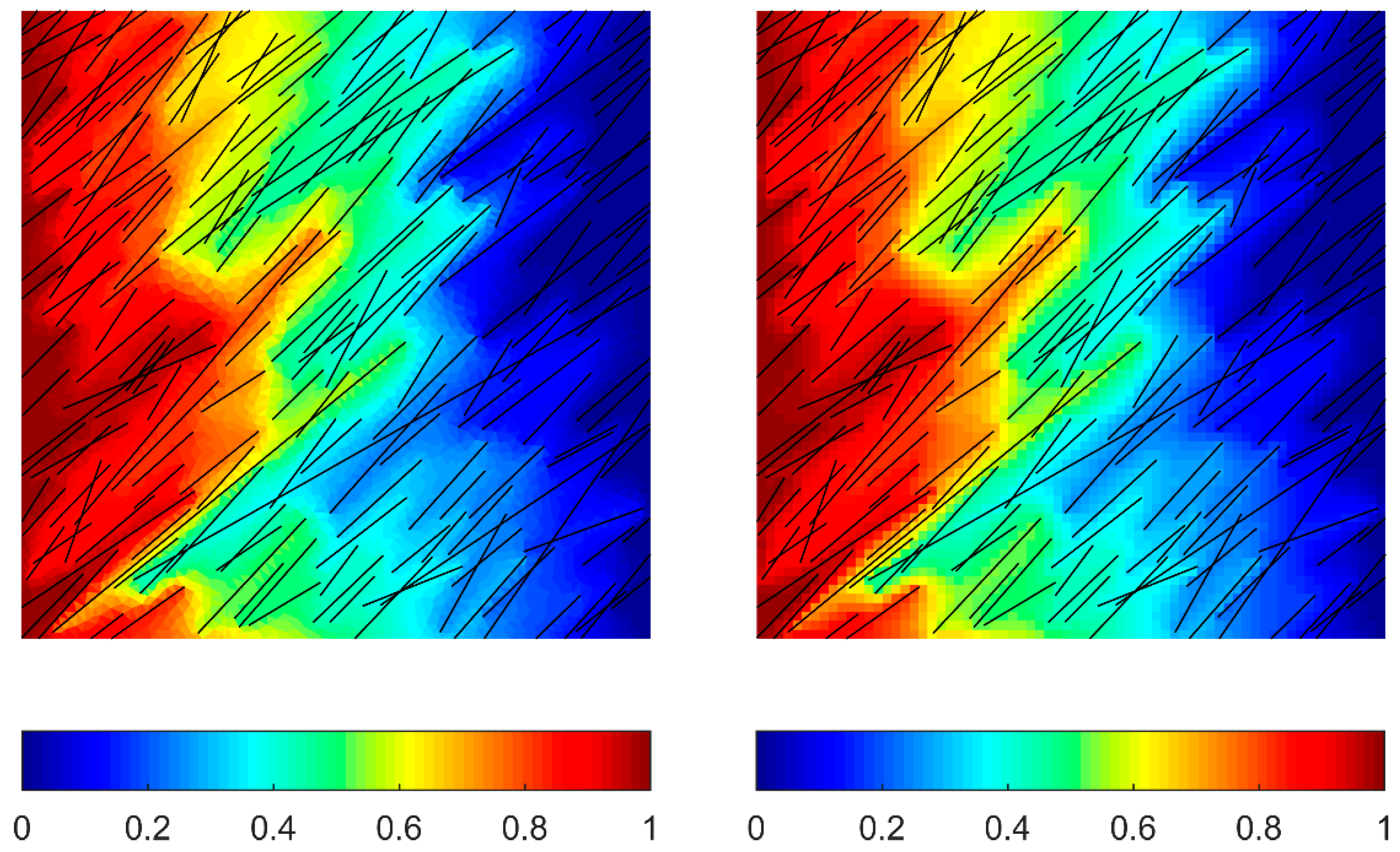
3. Results and Discussion

A series of numerical tests were conducted to assess the performance of the modeling workflow. Whenever possible, the reference solution was obtained by representing all the fractures in the given DFN explicitly using the EDFM method.

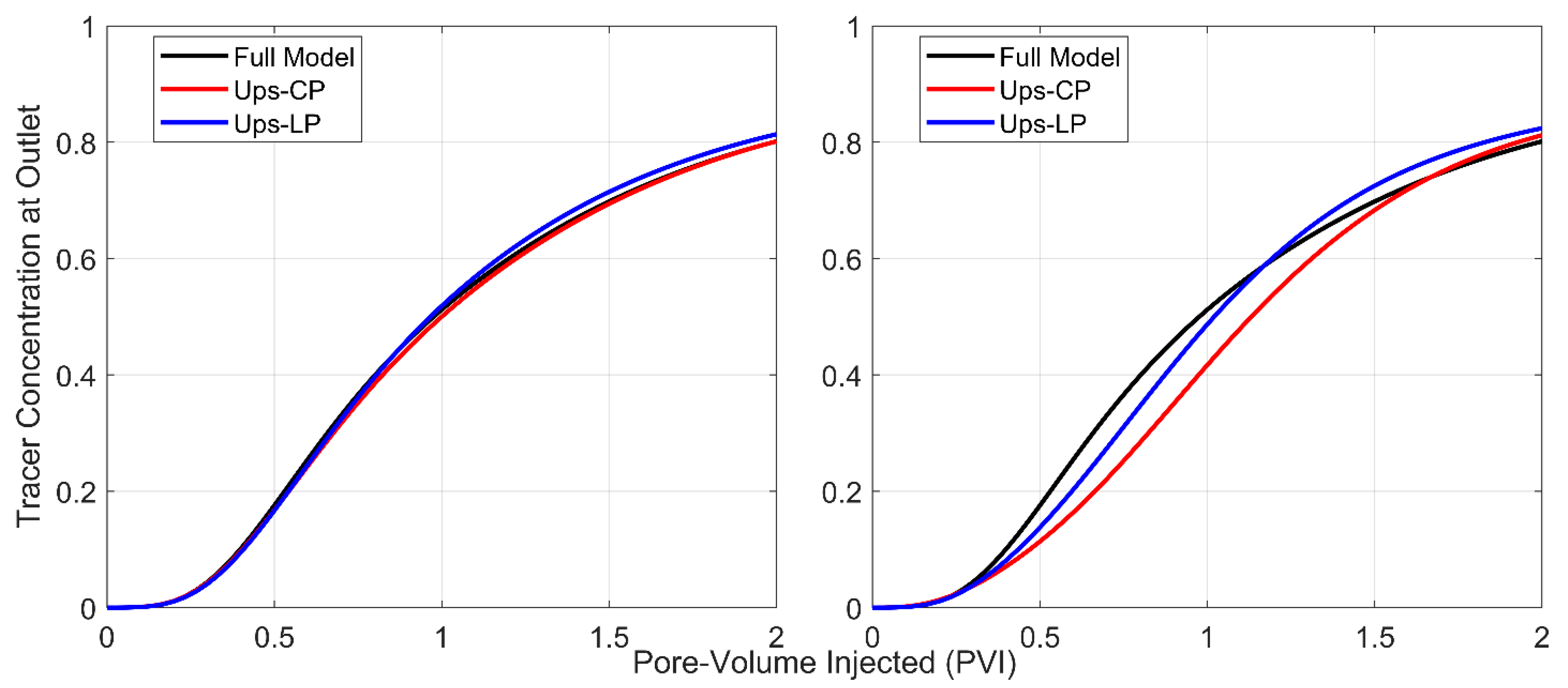
3.1. Case 1: Effect of Partition Length

In this first test, we established the base case and investigated the effect of partition length on the upscaled model. The reservoir domain was a square with dimensions $500 \mathrm{m}\times 500 \mathrm{m}$. The parameters used in this example are listed in

Table 2. Parameters for Case 1.

$\mathit{\mu }$	$\mathit{\pi }/4$	$\mathit{a}$	$5\times {10}^{-4} \mathbf{m}$
$\kappa$	50	$k_f$	$2.11\times {10}^7$ md
$\alpha$	2.5	${\varphi }_f$	0.8
$l_{\min }$	5 m	$k_m$	10 md
$l_{\max }$	500 m	${\varphi }_m$	0.2

. The left plot of Figure 5 shows one realization of the DFN generated using the given parameters and the right plot of the figure shows the length distribution of the fractures. The actual minimum and maximum fracture lengths were 2.95 m and 360.35 m, respectively, spanning two orders of magnitude. The DFN had a predominant orientation of ${45}^{°}$ counterclockwise rotation with respect to the $x$-axis. The total number of fractures in the DFN was 2995. All the fractures had the same aperture $a$, and fracture permeability is given by the following:

$$k_f=\frac{a^2}{12}$$

(9)

The rock matrix was assumed to be homogeneous and isotropic. To drive the global flow, Dirichlet boundary conditions of 10 MPa were imposed on the bottom left and 5 MPa on the upper right. The reservoir was meshed by a uniform $50\times 50$ Cartesian grid. The median of fracture lengths was 7.68 m, meaning that more than half of the fractures had lengths smaller than the characteristic length of the grid. The reference solution was obtained by modeling all the fractures explicitly using the EDFM method. The left plot of Figure 6 shows the reference pressure solution, and the tracer concentration solution after two pore-volume injection (2 PVI) is shown in the right plot of the figure.

To upscale the small-scale fractures, different partition lengths $l_{\mathrm{p}}$ were chosen. A smaller value of $l_{\mathrm{p}}$ means that more fractures are modeled explicitly. Since the upscaling of fractured porous media is tightly related to the size of the domain to be upscaled, we chose the value of $l_{\mathrm{p}}$ based on the characteristic length of the grid $l_{\mathrm{g}}$, as indicated in

Table 3. Partition length for upscaling and the corresponding percentage of fractures modeled explicitly.

$\mathbf{Partition} \mathbf{Length} {\mathit{l}}_{\mathbf{p}}$	% of Fractures Modeled Explicitly
$1\times l_{\mathrm{g}}$	28.38
$2\times l_{\mathrm{g}}$	9.68
$4\times l_{\mathrm{g}}$	3.37
$6\times l_{\mathrm{g}}$	1.97
$8\times l_{\mathrm{g}}$	1.04

. When the value of $l_{\mathrm{p}}$ is at its largest, only about 1% of fractures are modeled explicitly. Figure 7 shows the relative error of the pressure solutions of the two models, Ups-CP and Ups-LP, for two different partition lengths. It can be seen that when the partition length is small ($l_{\mathrm{p}}=l_{\mathrm{g}}$ in the first row), the two models have similar performance in terms of pressure solutions with the maximum relative error less than 1.5%. For a large partition length ($l_{\mathrm{p}}=8\times l_{\mathrm{g}}$ in the second row), however, the Ups-LP model performs much better than the Ups-CP model. This can be explained by the fact that when the partition length is smaller than or equal to the characteristic length of the grid, most of the upscaled fractures are contained inside a grid block and their effect on flow is local. Since the rock matrix is homogeneous and isotropic, an upscaled diagonal tensor is adequate to represent the combined flow behavior of the rock matrix and the fractures contained inside it. As the partition length increases, more fractures need to be upscaled with many fractures intersecting domain boundaries. The predominant orientation of the DFN means that the flow has a more pronounced anisotropic behavior at the grid-block scale and a full tensor is more appropriate to represent the fracture media at the scale of interest.

Figure 8 shows the absolute error of the tracer concentration after 2 PVI, and Figure 9 shows the tracer concentration at the outlet as a function of PVI for the two models with the two partition lengths. We can see that, for a small partition length ($l_{\mathrm{p}}=l_{\mathrm{g}}$), the errors of concentration distributions are generally small for both models with the Ups-CP model performing slightly better than the Ups-LP model compared to the reference solution. As the partition length $l_{\mathrm{p}}$ increases to $8\times l_{\mathrm{g}}$, the absolute error of concentration solution also increases for both models as more fractures are homogenized. However, the concentration solution using the Ups-LP model lies closer to the reference solution than the Ups-CP model, which is consistent with observations made about the pressure solutions. Figure 10 further shows the tracer breakthrough curves at the outlet for various partition lengths for the two models. For both models, there is a general tendency for the solutions to converge to the full model solution, i.e., the reference solution, with the Ups-CP model being more sensitive to the partition length. This test case suggests that, when the partition length is small (for example, comparable to the characteristic length of the grid), the Ups-CP model should be used as it is sufficiently accurate and computationally more efficient. For large partition values, the Ups-LP model should be used when the DFN has a predominant orientation as it better captures the directional dependencies of the fracture system.

3.2. Case 2: Effect of Fracture Length Distribution

The previous case features a DFN in which more than half of the fractures have lengths smaller than the characteristic length of the grid blocks. For this example, we investigated the effect of fracture length distribution by considering a DFN whose minimum fracture length was larger than the characteristic length of the grid blocks. The parameters used for generating the DFN were the same as those listed in Table 2 with the exception of $l_{\min }$. The minimum length here was set to 20 m, which is about twice the size of the characteristic length of the grid. The left plot in Figure 11 shows the generated DFN used in the following simulations, and its histogram of fracture length distribution is shown in the right of the figure. Other parameters for the model setup were the same as the previous case. Figure 12 shows the pressure solution and tracer concentration distribution after 2 PVI for the full model where all the fractures are modeled explicitly using the EDFM method. Unsurprisingly, the system displays a strong preferential orientation for flow and transport because of the presence of the fracture network. For illustration purposes, we first upscaled all the fractures on a $8\times 8$ Cartesian grid using the two different upscaling methods, and the results are shown in Figure 13. As expected, Ups-CP produces diagonal tensors, whereas the upscaled tensors from Ups-LP have principal directions aligned with the predominant direction of the underlying DFN. Next, a partition length of $l_{\mathrm{p}}=5\times l_{\mathrm{g}}$ was chosen so that about 10% of the largest fractures were modeled explicitly, whereas the remaining fractures were upscaled with the rock matrix. Figure 14 and Figure 15 display the relative error of the pressure solutions and the absolute error of tracer concentration distribution after 2 PVI for the Ups-CP and Ups-LP models, respectively. Figure 14 shows that the relative error of the pressure solutions using the Ups-LP model is significantly smaller than that using the Ups-CP model, suggesting that the Ups-LP model is much more effective in capturing the directional dependencies of the pressure solution caused by the underlying fracture network. The absolute error of the concentration solution shown in Figure 15 show that the Ups-LP model performs modestly better than the Ups-CP model, but the breakthrough curves of tracers at the outlet depicted in Figure 16 shows that the results of Ups-LP are much closer to the reference solution compared to those of the Ups-CP model. The results of this case are in line with the observations made from the first case in that the Ups-LP model is more appropriate for upscaling fractured media when the underlying DFN has a predominant orientation and the upscaled fractures are larger than the characteristic length of the grid. Since the minimum length of the discrete fractures is larger than the characteristic length of the underlying grid, the fractures to be upscaled generally cut through the hosting grid block, which, combined with the fact that the fracture network has a predominant orientation, means that the Ups-LP model has superior performance compared to the Ups-CP model.

3.3. Case 3: Effect of Fracture Orientation

For this case, we investigated the effect of fracture orientation on the performance of the two upscaling methods. The parameters used for generating the DFN are the same as those listed in Table 2 except that the parameter $\kappa$ takes the value of 1. As mentioned in Section 2.2, the parameter $\kappa$ controls the variance of the fracture orientations. A small value of 1 gives an orientation distribution that has large variance. Figure 17 shows the corresponding DFN used in the following simulations together with the histogram of the length distribution. As can be seen from the figure, the DFN does not have a particular predominant orientation. Similarly, the reference solution is obtained by modeling all the fractures explicitly using the EDFM method, and the results are given in Figure 18, which shows that the pressure diffuses more uniformly from the injection inlet to the production outlet and the distribution of tracer concentration is also more random compared to the previous two cases. Figure 19 and Figure 20 show the relative errors of pressure solutions and absolute errors of tracer concentration solutions after 2 PVI, respectively, for the two upscaling models, Ups-CP and Ups-LP. For this case, the Ups-CP model shows better performance in terms of pressure solutions over the Ups-LP model as can be seen in Figure 19, but conclusions about the transport solutions are less definitive from Figure 20. Furthermore, there is no obvious winner that performs significantly better than the other, although the breakthrough curves depicted in Figure 21 suggest that the flux solution of Ups-LP is closer to the reference solution than that of Ups-CP. Different realizations of the DFN were generated using the same parameters and additional simulations were carried out on these DFNs. Our findings indicated that the opposite scenario can also occur; that is, for some realizations of the DFN, Ups-LP gives more accurate pressure solutions but less accurate flux solutions than Ups-CP compared to the reference solution. Therefore, no definite conclusions can be reached about which one is better when the DFN does not have predominant orientations.

4. Summary and Conclusions

A general workflow for modeling flow and transport in fractured porous media was introduced in this work. Based on a given partition length l_p, fractures were classified as small-scale fractures (fractures with lengths smaller than l_p) and large-scale fractures (fractures with lengths greater than l_p). The small-scale fractures were upscaled with the hosting matrix, whereas the large-scale fractures were modeled explicitly using the EDFM model. A hybrid upscaling approach was proposed that switches between applying the linearly varying pressure boundary condition and the constant pressure drop boundary condition. The linearly varying pressure boundary condition was preferentially applied to capture the anisotropic effect of the fracture porous media. If the resulting upscaled permeability tensor was not positive-definite, the constant pressure drop boundary condition was used instead to produce an upscaled tensor that was diagonal. Once the small-scale fractures were upscaled, the original fractured reservoir was replaced by an equivalent medium with large-scale fractures embedded in it. Our numerical results suggest that when the partition length is comparable to the characteristic length of the grid blocks or the DFN does not have a predominant orientation, the Ups-CP model should be the method of choice as it is computationally more efficient and has similar accuracy compared to the Ups-LP model. The Ups-LP model is best suited for cases in which the small-scale fractures to be upscaled cut through the grid block and have a predominant orientation.

The current workflow implementation homogenizes the small-scale fractures and the porous matrix into a single medium. An alternative is to upscale only the small-scale fractures into a distinct continuum of its own, leading to dual-continuum models while the large-scale fractures are still modeled explicitly. A comparison between the single-continuum upscaling and the dual-continuum upscaling would be of great interest for obtaining a complete picture of modeling small-scale fractures. Moreover, the current work focuses on single-phase flow. A future extension could include multi-phase flow along with its intertwined complex flow dynamics.

References

1. Berre, I.; Doster, F.; Keilegavlen, E. Flow in Fractured Porous Media: A Review of Conceptual Models and Discretization Approaches. Transp. Porous Media 2019, 130, 215–236. [Google Scholar] [CrossRef] [Green Version]
2. Barenblatt, G.I.; Zheltov, I.P.; Kochina, I.N. Basic concepts in the theory of seepage of homogeneous liquids in fissured rocks [strata]. J. Appl. Math. Mech. 1960, 24, 1286–1303. [Google Scholar] [CrossRef]
3. Warren, J.E.; Root, P.J. The Behavior of Naturally Fractured Reservoirs. Soc. Pet. Eng. J. 1963, 3, 245–255. [Google Scholar] [CrossRef] [Green Version]
4. Kazemi, H.; Merrill, L.S., Jr.; Porterfield, K.L.; Zeman, P.R. Numerical Simulation of Water-Oil Flow in Naturally Fractured Reservoirs. Soc. Pet. Eng. J. 1976, 16, 317–326. [Google Scholar] [CrossRef]
5. Thomas, L.K.; Dixon, T.N.; Pierson, R.G. Fractured Reservoir Simulation. Soc. Pet. Eng. J. 1983, 23, 42–54. [Google Scholar] [CrossRef]
6. Dean, R.H.; Lo, L.L. Simulations of Naturally Fractured Reservoirs. SPE Reserv. Eng. 1988, 3, 638–648. [Google Scholar] [CrossRef]
7. Kazemi, H.; Gilman, J.R.; Elsharkawy, A.M. Analytical and Numerical Solution of Oil Recovery from Fractured Reservoirs with Empirical Transfer Functions (includes associated papers 25528 and 25818). SPE Reserv. Eng. 1992, 7, 219–227. [Google Scholar] [CrossRef]
8. Lim, K.T.; Aziz, K. Matrix-fracture transfer shape factors for dual-porosity simulators. J. Pet. Sci. Eng. 1995, 13, 169–178. [Google Scholar] [CrossRef]
9. Heinemann, Z.E.; Mittermeir, G.M. Rigorous Derivation of the Kazemi-Gilman-Elsharkawy Generalized Dual Porosity Shape Factor. Transp. Porous Media 2006. [Google Scholar] [CrossRef]
10. Geiger, S.; Roberts, S.; Matthäi, S.K.; Zoppou, C.; Burri, A. Combining finite element and finite volume methods for efficient multiphase flow simulations in highly heterogeneous and structurally complex geologic media. Geofluids 2004, 4, 284–299. [Google Scholar] [CrossRef]
11. Karimi-Fard, M.; Durlofsky, L.J.; Aziz, K. An Efficient Discrete-Fracture Model Applicable for General-Purpose Reservoir Simulators. SPE J. 2004, 9, 227–236. [Google Scholar] [CrossRef]
12. Li, L.; Lee, S.H. Efficient Field-Scale Simulation of Black Oil in a Naturally Fractured Reservoir through Discrete Fracture Networks and Homogenized Media. SPE Reserv. Eval. Eng. 2008, 11, 750–758. [Google Scholar] [CrossRef]
13. Moinfar, A.; Varavei, A.; Sepehrnoori, K.; Johns, R.T. Development of an Efficient Embedded Discrete Fracture Model for 3D Compositional Reservoir Simulation in Fractured Reservoirs. SPE J. 2014, 19, 289–303. [Google Scholar] [CrossRef] [Green Version]
14. Lee, S.H.; Jensen, C.L.; Lough, M.F. Efficient Finite-Difference Model for Flow in a Reservoir With Multiple Length-Scale Fractures. SPE J. 2000, 5, 268–275. [Google Scholar] [CrossRef]
15. Lee, S.H.; Lough, M.F.; Jensen, C.L. Hierarchical modeling of flow in naturally fractured formations with multiple length scales. Water Resour. Res. 2001, 37, 443–455. [Google Scholar] [CrossRef]
16. Wong, D.L.Y.; Doster, F.; Geiger, S.; Kamp, A. Partitioning Thresholds in Hybrid Implicit-Explicit Representations of Naturally Fractured Reservoirs. Water Resour. Res. 2020, 56, e2019WR025774. [Google Scholar] [CrossRef]
17. Zhang, W.; Al Kobaisi, M. Cell-Centered Nonlinear Finite-Volume Methods with Improved Robustness. SPE J. 2020, 25, 288–309. [Google Scholar] [CrossRef]
18. Berens, P. CircStat: A MATLAB Toolbox for Circular Statistics. J. Stat. Softw. 2009, 31, 1–21. [Google Scholar] [CrossRef] [Green Version]
19. Clauset, A.; Shalizi, C.R.; Newman, M.E.J. Power-Law Distributions in Empirical Data. SIAM Rev. 2009, 51, 661–703. [Google Scholar] [CrossRef] [Green Version]
20. Durlofsky, L.J. Upscaling and gridding of fine scale geological models for flow simulation. In Proceedings of the 8th International Forum on Reservoir Simulation Iles Borromees, Stresa, Italy, 20–24 June 2005; pp. 1–59. [Google Scholar]
21. Zhang, W.; Al Kobaisi, M. Discrete Fracture-Matrix Simulations Using Cell-Centered Nonlinear Finite Volume Methods. In ECMOR XVII; European Association of Geoscientists & Engineers: Edinburgh, UK, 2020. [Google Scholar]
22. Zhang, W.; Al Kobaisi, M. Nonlinear finite volume method for 3D discrete fracture-matrix simulations. SPE J. 2020. [Google Scholar] [CrossRef]
Figure 1. Workflow for modeling fractures with multiple length scales.
Energies 13 06667 g001
Figure 2. Boundary conditions used for numerical upscaling. (Left) constant pressure drop (CP) on a pair of opposing faces and no-flow boundary conditions on the remaining faces (Ups-CP). (Right) linear pressure (LP) conditions on all boundary faces (Ups-LP).
Energies 13 06667 g002
Figure 3. Discrete fracture network (left) and unstructured triangular mesh with 11,448 elements conforming to the fracture geometries (right).
Energies 13 06667 g003
Figure 4. Pressure distribution using DFM-NTPFA (left) using 11,448 elements and EDFM-TPFA (right) using 4900 elements (i.e., 70 × 70 ) blocks.
Energies 13 06667 g004
Figure 5. (Left) DFN on a square domain with dimension 500 m × 500 m. (Right) Histogram of fracture length distribution.
Energies 13 06667 g005
Figure 6. Reference solution for pressure distribution (left) and tracer concentration distribution after two pore-volume injection (2 PVI) (right).
Energies 13 06667 g006
Figure 7. Relative error of pressure solutions for the Ups-CP (first column) and Ups-LP (second column) models when the partition is l p = l g (first row) and l p = 8 × l g (second row).
Energies 13 06667 g007
Figure 8. Absolute error of the tracer concentration solutions after 2 PVI for the Ups-CP (first column) and Ups-LP (second column) models when the partition is l p = l g (first row) and l p = 8 × l g (second row).
Energies 13 06667 g008
Figure 9. Tracer concentration at the outlet as a function of pore-volume injected for full model, Ups-CP, and Ups-LP for l p = l g (left) and l p = 8 × l g (right).
Energies 13 06667 g009
Figure 10. Tracer concentration at the outlet as a function of pore-volume injected using different partition lengths l p for Ups-CP (left) and Ups-LP (right).
Energies 13 06667 g010
Figure 11. DFN for Case 2 (left) and its histogram of the fracture length distribution (right).
Energies 13 06667 g011
Figure 12. Reference pressure solution (left) and tracer concentration distribution after 2 PVI (right).
Energies 13 06667 g012
Figure 13. Upscaled permeability tensor represented by ellipses whose semi-axes are scaled by the square root of the principal values. (Left) Ups-CP; (right) Ups-LP.
Energies 13 06667 g013
Figure 14. Case 2: relative error of pressure solutions for Ups-CP (left) and Ups-LP (right).
Energies 13 06667 g014
Figure 15. Case 2: absolute error of tracer concentration for Ups-CP (left) and Ups-LP (right).
Energies 13 06667 g015
Figure 16. Case 2: tracer concentration at the outlet as a function of pore-volume injected.
Energies 13 06667 g016
Figure 17. Case 3: DFN (left) and its histogram of the fracture length distribution (right).
Energies 13 06667 g017
Figure 18. Case 3: reference solution for pressure distribution (left) and tracer concentration distribution after 2 PVI (right).
Energies 13 06667 g018
Figure 19. Case 3: relative error of pressure solutions for Ups-CP (left) and Ups-LP (right).
Energies 13 06667 g019
Figure 20. Case 3: absolute error of tracer concentration for Ups-CP (left) and Ups-LP (right).
Energies 13 06667 g020
Figure 21. Case 3: tracer concentration at the outlet as a function of pore-volume injected.
Energies 13 06667 g021